Accurate statistics of a flexible polymer chain in shear flow.

Abstract

We present exact and analytically accurate results for the problem of a flexible polymer chain in shear flow. Under such a flow the polymer tumbles, and the probability distribution of the tumbling times $\tau$ of the polymer decays exponentially as $\sim\exp(-\alpha\tau/\tau_{0})$ (where $\tau_{0}$ is the longest relaxation time). We show that for a Rouse chain, this nontrivial constant $\alpha$ can be calculated in the limit of large Weissenberg number (high shear rate) and is in excellent agreement with our simulation result of $\alpha\simeq 0.324$. We also derive exactly the distribution functions for the length and the orientational angles of the end-to-end vector $\boldsymbol{R}$ of the polymer.

Dynamics of a polymer under a shear flow has been of great interest both experimentally and theoretically gennes ; chu ; LeDuc ; smith ; doyle ; dua ; chertkov ; puliafito ; celani ; gera ; winkler ; bhatt . In biological systems, biomolecules subjected to complex fluid flows chu1 ; dua are quite common, and a shear flow is one such example. In shear flow, a polymer gets stretched as well as tumbles in an irregular fashion. A crucial quantity which describes the interesting conformational evolution of the polymer is its end-to-end vector $\boldsymbol{R}$ (see Fig. 1). Recently, experiments on a single DNA molecule in shear flow gera have obtained accurate probability distribution functions of the length, the orientational angles, and the tumbling times of the vector $\boldsymbol{R}$. On the other hand, theoretically, although scaling results from studies of non-linear single bead-spring model chertkov ; celani ; puliafito and approximate analysis of semi-flexible chains winkler are known, these are mostly non-exact.

For a non-linear system as a semi-flexible polymer (like DNA), approximate theoretical results as in chertkov ; winkler are perhaps as best as one can get. They agree well with the static properties seen in experiments gera . On the other hand, exact and analytically accurate results are very desirable for at least the flexible polymer problem. In particular, there exists no theory for the tumbling time statistics of the vector $\boldsymbol{R}$; heuristic arguments given in chertkov ; winkler are simply inadequate, as will be evident from our analysis below. In this Letter, we derive exact and analytically accurate results for the static and dynamic properties of $\boldsymbol{R}$ of a flexible Rouse chain Rouse in shear flow.

The stochastic process of our concern, namely the end-to-end vector $\boldsymbol{R}(t)$ of a linear polymer is a Gaussian random variable and its dynamics is non-Markovian. The aspect of Gaussianity makes it quite easy to write down the static “joint” probability density function (PDF) of the Cartesian components of the vector $\boldsymbol{R}$, and consequently the joint PDF of the length $R$, latitude angle $\theta$ and the azimuthal angles $\phi$ puliafito ; winkler . The first non-triviality is to get the PDFs of the individual polar co-ordinates, namely, $F(R)$, $U(\theta)$ and $Q(\phi)$, in the stationary state. While $Q(\phi)$ was known puliafito ; winkler , in this Letter we derive $F(R)$ and $U(\theta)$ exactly for a linear chain.

Figure 1: A polymer configuration with shear flow along $x$-direction.

Secondly, the non-Markovian evolution of $\boldsymbol{R}(t)$ multi_Markov makes the first-passage questions (like the tumbling time statistics) analytically extremely challenging. First passage questions in the context of polymers have been of long standing interest fixman ; doi ; marques . In general, for non-Markovian processes, calculation of first-passage properties are very nontrivial even when the full knowledge of the non-exponential two-time correlation function is available McFadden ; Review ; satya ; satya2 . However, when a process is smooth (as defined below) a method called ‘Independent interval approximation’ (IIA) is applicable McFadden and yields accurate estimates satya2 ; bhatt . Very interestingly, while in the absence of shear any component of $\boldsymbol{R}(t)$ is a non-smooth process and thus analytical prediction is unknown, we show below that in the presence of strong shear, a suitable component of $\boldsymbol{R}(t)$ associated with tumbling becomes a smooth process, leading to analytical tractability via IIA. Thus quite unexpectedly mathematical simplicity is achieved in a case of greater physical complexity. To be precise, we show that the PDF of “angular tumbling times” $\tau$, goes as $\sim\exp{(-{\alpha\tau/\tau_{0}})}$ (where $\tau_{0}$ is the longest relaxation time of the chain), and in the limit of large shear rate $\alpha\rightarrow 0.324^{+}$. This number will serve as a lower bound for experiments.

As shown in Fig. 1, we study the Rouse dynamics Rouse ; edwards of a polymer chain of $N$ beads connected by harmonic springs, in a shear flow in the $x$-direction. Let $\boldsymbol{r}_{n}(t)\equiv[x_{n}(t),y_{n}(t),z_{n}(t)]^{T}$ denote the coordinate vector of the $n^{\text{th}}$ bead ($n=1,2,\dotsc,N)$ at time $t$. For $n=2,3,\dotsc,N-1$, the position vectors evolve with time according to the equation of motion

$$\frac{\mathrm{d}\boldsymbol{r}_{n}}{\mathrm{d}t}=k\left(\boldsymbol{r}_{n+1}+\boldsymbol{r}_{n-1}-2\,\boldsymbol{r}_{n}\right)+\boldsymbol{f}_{n}(t)+\boldsymbol{\eta}(n,t),$$ (1)

where $k$ denotes the strength of the harmonic interaction between nearest neighbor beads, and the vector $\boldsymbol{f}_{n}(t)\equiv[\dot{\gamma}y_{n}(t),0,0]^{T}$ denotes the shear force field with rate $\dot{\gamma}$. The Weissenberg number $\mathrm{Wi}=\dot{\gamma}\tau_{0}$, where the longest relaxation time $\tau_{0}=N^{2}/{k\pi^{2}}$. The vector $\boldsymbol{\eta}(n,t)\equiv[\eta_{1}(n,t),\eta_{2}(n,t),\eta_{3}(n,t)]^{T}$ represents the thermal white noise with zero mean and a correlator $\langle\eta_{i}(n,t)\eta_{j}(n^{\prime},t^{\prime})\rangle=\zeta\delta_{ij}\delta_{n,n^{\prime}}\delta(t-t^{\prime}),$ where $i,j=1,2,3$ and $n,n^{\prime}=1,2,\dotsc,N$. The noise strength $\zeta$ is proportional to the temperature and all the force strengths in Eq. (1) are scaled by viscosity. With free boundary condition, the two end-beads (for $n=1$ and $n=N$) feel only one sided interaction and therefore they evolve via modified equations which is obtained from Eq. (1) by using $\boldsymbol{r}_{0}(t)=\boldsymbol{r}_{1}(t)$ and $\boldsymbol{r}_{N+1}(t)=\boldsymbol{r}_{N}(t)$, for two fictitious beads $0$ and $N+1$.

For large $N$ limit, the discrete $n$ of the beads is replaced by a continuous variable $s$ edwards and the discrete Laplacian in Eq. (1) is replaced by a continuous second derivative along $s$ direction. Equation (1) then leads to

$$\frac{\partial\boldsymbol{r}(s,t)}{\partial t}=k\frac{\partial^{2}\boldsymbol{r}(s,t)}{\partial s^{2}}+\boldsymbol{f}(s,t)+\boldsymbol{\eta}(s,t),$$ (2)

with the free boundary conditions $\partial\boldsymbol{r}(s,t)/\partial s=0$ at $s=0$ and $s=N$. In this continuum limit, the shear field and the noise correlator are given by $\boldsymbol{f}(s,t)\equiv[\dot{\gamma}y(s,t),0,0]^{T}$ and $\langle\eta_{i}(s,t)\eta_{j}(s^{\prime},t^{\prime})\rangle=\zeta\delta_{ij}\delta(s-s^{\prime})\delta(t-t^{\prime})$ respectively. The end-to-end vector is $\boldsymbol{R}(t)=\boldsymbol{r}(N,t)-\boldsymbol{r}(0,t)$.

Solving Eq. (2) by the Fourier cosine transformation

$$\boldsymbol{r}(s,t)=\tilde{\boldsymbol{r}}(0,t)+\sum_{m=1}^{\infty}\tilde{\boldsymbol{r}}(m,t)\cos\left(\frac{m\pi s}{N}\right),$$ (3)

we find that the Fourier modes are given by

$$\tilde{\boldsymbol{r}}(m,t)= \int_{0}^{t}\Bigl{[}\tilde{\boldsymbol{f}}(m,t^{\prime})+\tilde{\boldsymbol{\eta}}(m,t^{\prime})\Bigr{]}\,\exp\bigl{[}-a_{m}(t-t^{\prime})\bigr{]}\,\mathrm{d}t^{\prime}$$

$$+\tilde{\boldsymbol{r}}(m,0)\,\exp(-a_{m}t)$$ (4)

where $a_{m}=m^{2}/\tau_{0}$, and $\tilde{\boldsymbol{f}}(m,t)=[\dot{\gamma}\tilde{y}(m,t),0,0]^{T}$ and $\tilde{\boldsymbol{\eta}}(m,t)\equiv[\tilde{\eta_{1}}(m,t),\tilde{\eta_{2}}(m,t),\tilde{\eta_{3}}(m,t)]^{T}$ is the $m^{\text{th}}$ Fourier mode of the noise vector $\boldsymbol{\eta}(s,t)$. The zero mode $\tilde{\boldsymbol{r}}(0,t)=N^{-1}\int_{0}^{N}\boldsymbol{r}(s,t)\,\mathrm{d}s$ describes the center of mass motion of the polymer. Equations (3) and (4), together with the knowledge of the Fourier space noise correlator $\langle\tilde{\eta_{i}}(m,t)\tilde{\eta_{j}}(m^{\prime},t^{\prime})\rangle=2\zeta N^{-1}\delta_{ij}\delta_{m,m^{\prime}}\delta(t-t^{\prime}),$ after some algebra, leads to the two point space and time dependent correlation function between different relative position coordinates. In the stationary state limit $t\rightarrow\infty$ with a finite time increment $\tau\geq 0$, the correlation function

$$\bigl{\langle}[\boldsymbol{r}^{(i)}(s_{1},t)-\tilde{\boldsymbol{r}}^{(i)}(0,t)]\cdot[\boldsymbol{r}^{(j)}(s_{2},t+\tau)- \tilde{\boldsymbol{r}}^{(j)}(0,t+\tau)]\bigr{\rangle}$$

$$\xrightarrow{t\rightarrow\infty}\frac{2\zeta}{N}\sum_{m=1}^{\infty}\cos\left(\frac{m\pi s_{1}}{N}\right)\cos\left(\frac{m\pi s_{2}}{N}\right) \times$$

$$\biggr{[}\delta_{i1}\delta_{j1}{\dot{\gamma}}^{2}\left(\frac{2\mathrm{e}^{-a_{m}\tau}}{(2a_{m})^{3}}+\frac{\tau\mathrm{e}^{-a_{m}\tau}}{(2a_{m})^{2}}\right)+ \delta_{ij}\frac{\mathrm{e}^{-a_{m}\tau}}{(2a_{m})}$$

$$+\delta_{i1}\delta_{j2}\dot{\gamma}\left(\frac{\mathrm{e}^{-a_{m}\tau}}{(2a_{m})^{2}}+\frac{\tau\mathrm{e}^{-a_{m}\tau}}{(2a_{m})}\right) \biggr{]},$$ (5)

where ${i,j}={1,2,3}$ and the notations $\boldsymbol{r}^{(1)}(s,t)\equiv x(s,t)$, $\boldsymbol{r}^{(2)}(s,t)\equiv y(s,t)$, and $\boldsymbol{r}^{(3)}(s,t)\equiv z(s,t)$. Note that, any static correlation function in the stationary state limit can be obtained by setting $\tau=0$ in the above equation. On the other hand, for dynamic properties like tumbling, we need the correlators with $\tau>0$.

We first consider the static distribution functions related to $\boldsymbol{R}\equiv[R_{x},R_{y},R_{z}]^{T}$. Since the Cartesian components are Gaussian random variables, their joint PDF is, ${\cal{P}}(R_{x},R_{y},R_{z})=(2\pi)^{-3/2}|\boldsymbol{C}|^{-1/2}\exp(-\frac{1}{2}\boldsymbol{R}^{T}\boldsymbol{C}^{-1}\boldsymbol{R}),$ where $\boldsymbol{C}$ denotes the covariance matrix. Putting $\tau=0$ and $(s_{1},s_{2})=(0,0),(0,N),(N,0)$ and $(N,N)$ in Eq. (5) we get the four correlators, respectively, needed to calculate each elements of $\boldsymbol{C}$. Since the vector $\boldsymbol{R}$ is a difference of two position coordinates, the zero modes cancel, and hence we need not worry about it being present in Eq. (5). We find,

$$\boldsymbol{C}\equiv\left[\begin{array}[]{ccc}\langle R_{x}^{2}\rangle&\langle R_{x}R_{y}\rangle&\langle R_{x}R_{z}\rangle\\ \langle R_{x}R_{y}\rangle&\langle R_{y}^{2}\rangle&\langle R_{y}R_{z}\rangle\\ \langle R_{x}R_{z}\rangle&\langle R_{y}R_{x}\rangle&\langle R_{z}^{2}\rangle\end{array}\right]=\left[\begin{array}[]{ccc}d&b&0\\ b&a&0\\ 0&0&a\end{array}\right],$$ (6)

where

$$a=\frac{\zeta N}{2k},\quad b=\frac{\zeta N\pi^{2}}{48k}\mathrm{Wi},\quad d=a+\frac{\zeta N\pi^{4}}{480k}\mathrm{Wi}^{2},$$ (7)

and the determinant $|\boldsymbol{C}|=ac$, with $c=ad-b^{2}$.

The scaling of $\langle R_{x}^{2}\rangle=d\approx N\mathrm{Wi}^{2}\sim N^{5}$ is a pathological feature of the Rouse model in shear flow in comparison to semi-flexible polymers (better modeled with FENE constraint on $\boldsymbol{R}$ dua ). If the $\mathrm{Wi}$ dependencies are ignored, the asymptotic functional forms of the PDF’s of the Rouse model, compare quite well with semi-flexible polymers.

It is straightforward to obtain the joint PDF of the polar coordinates by using the standard transformation: $\tilde{\cal P}(R,\theta,\phi)={\cal P}(R\cos\theta\cos\phi,R\cos\theta\sin\phi,R\sin\theta)R^{2}\cos\theta$. By integrating it over $R$ we get the joint angular PDF

$$S(\theta,\phi)= \frac{|\boldsymbol{C}|\cos\theta}{4\pi}\bigl{[}a\cos^{2}\theta\bigl{\{}a\cos^{2}\phi+d\sin^{2}\phi$$

$$- 2b\sin\phi\cos\phi\bigr{\}}+c\sin^{2}\theta\bigr{]}^{-{3/2}}.$$ (8)

Now again integrating over $\phi$ in Eq. (8), we obtain our first important result, the PDF of the latitude angle,

$$U(\theta)=\frac{|\boldsymbol{C}|\cos{\theta}}{\pi(d_{1}-d_{2})\sqrt{d_{1}+d_{2}}}\;\mathbf{E}\left(\sqrt{\frac{2d_{2}}{d_{1}+d_{2}}}\right),$$ (9)

where $d_{1}=[a(d+a)/2]\cos^{2}\theta+c\sin^{2}\theta$, $d_{2}=(a/2)[(d-a)^{2}+4b^{2}]^{1/2}\cos^{2}\theta$, and $\mathbf{E}(q)=\int_{0}^{\pi/2}\bigl{(}1-q^{2}\sin^{2}\beta\bigr{)}^{1/2}\mathrm{d}\beta$ is the complete elliptic integral of second kind grad . From our exact result in Eq. (9), by taking the limit of $\dot{\gamma}\gg 1$ and $\theta\ll 1$, we see that the $\mathbf{E}(.)\rightarrow{\rm constant}$, and $(d_{1}+d_{2})\approx ad$ and $(d_{1}-d_{2})\approx c\theta^{2}$: these lead to $U(\theta)\sim\mathrm{Wi}^{-1}\theta^{-2}$. Further, from Eq. (8), in the same limit $S(\phi=0,\theta)\sim\mathrm{Wi}^{-1}\theta^{-3}$. The azimuthal angle distribution $Q(\phi)=\int_{-\pi/2}^{\pi/2}S(\theta,\phi)\,\mathrm{d}\theta$ can be easily derived from Eq. (8); we skip its explicit expression as similar result has been derived earlier in puliafito ; winkler . We just note that $Q(\phi)$ peaks exactly at $\phi=\phi_{m}=\frac{1}{2}\tan^{-1}\left(\frac{2b}{d-a}\right).$ The full width at half maximum $\Delta\phi$ of $Q(\phi)$ is given exactly by $\cos(2\Delta\phi)=2-[(d+a)/(d-a)]\cos{2\phi_{m}}$ and for $\dot{\gamma}\gg 1$, $\Delta\phi\approx\phi_{m}\sim\mathrm{Wi}^{-1}$ and $Q(\phi)\approx\mathrm{Wi}^{-1}\sin^{-2}\phi.$ The asymptotic dependences of the functions $U(\theta)$, $S(\phi=0,\theta)$ and $Q(\phi)$ on $\theta$ and $\phi$, that we derive from our exact Eqs. (8) and (9) for a Rouse polymer, match with earlier studies on semi-flexible polymers chertkov ; puliafito ; celani ; winkler ; gera .

To derive our second result for the radial length distribution function $F(R)=\int_{0}^{2\pi}\mathrm{d}\phi\int_{-\pi/2}^{\pi/2}\mathrm{d}\theta\,\tilde{\cal P}(R,\theta,\phi),$ we employ the trick of first calculating the Laplace transform of the PDF of $R^{2}$ instead, namely $h(s)\equiv\langle\exp(-sR^{2})\rangle=\langle\exp\bigl{(}-s[R_{x}^{2}+R_{y}^{2}+R_{z}^{2}]\bigr{)}\rangle.$ This is easily obtained as $h(s)=\bigl{(}1+2as\bigr{)}^{-1/2}\,\bigl{(}1+2s(a+d)+4cs^{2}\bigr{)}^{-1/2}.$ The PDF $F(R)$ is then related to the the inverse Laplace transform of $h(s)$ as $F(R)=2R\times\left[\mathcal{L}_{s}^{-1}\{h(s)\}(R^{2})\right]$ and is given exactly as

$$F(R)=\frac{R^{2}\mathrm{e}^{-R^{2}/{2a}}}{\sqrt{2\pi|\boldsymbol{C}|}}\int_{0}^{1}\mathrm{d}x\frac{\mathrm{e}^{\lambda R^{2}x}I_{0}(\mu R^{2}x)}{\sqrt{1-x}},$$ (10)

where $I_{0}(.)$ is zeroth order modified Bessel function of first kind grad , and $\lambda=1/(2a)-(a+d)/(4c)$ and $\mu=\sqrt{(d-a)^{2}+4b^{2}}/(4c).$ From asymptotic analysis of Eq. (10) we see that $F(R)\approx\sqrt{2}R^{2}\big{/}\sqrt{\pi|\boldsymbol{C}|}$ for small $R$, and $F(R)\approx\exp\bigl{(}-[1/(2a)-\lambda-\mu]R^{2}\bigr{)}\big{/}{\sqrt{4\pi|\boldsymbol{C}|\mu(\mu+\lambda)}}$ for large $R$.

We now turn our attention to our third and main result on the first passage question of the polymer “tumbling” process in shear flow. The tumbling event is either defined as a radial return of the polymer to a coiled state (as in experiments gera and simulations celani ), or as a angular return of vector $\boldsymbol{R}$ to a fixed plane celani , say $\phi=0$. The former radial definition relies on an arbitrary choice of a threshold radius gera ; celani , while the latter angular tumbling is not. In this Letter we study the statistics of angular tumbling time, i.e. the distribution of times $\tau$ between two successive zero crossings of the stochastic process $R_{x}(t)$. For the scaled time $T=\tau/\tau_{0}$ the relevant PDF asymptotically is $P(T)\sim\exp(-\alpha T).$ Analytical scaling dependence of $\alpha$ on $\mathrm{Wi}$ is known for semi-flexible polymers chertkov , but accurate constant factors were not estimated. We show below that for a Rouse chain, in the limit of large $\mathrm{Wi}$, $\alpha$ approaches a constant value, and that can be estimated by using a systematic IIA calculation.

For a Gaussian stationary process, the mean density of zero crossings is given by rice : $\rho=1/\langle T\rangle=\sqrt{-A^{\prime\prime}(0)}/\pi$, where $A(T)$ is the normalized correlator, i.e., $A(0)=1$. We need $A^{\prime}(0)=0$ and a finite $A^{\prime\prime}(0)$ for $\rho$ to be finite —then the process is smooth and one can use IIA McFadden .

Now, for the relevant stochastic process $R_{x}(t)$ of our concern, using Eq. (5) we find the stationary state correlator $C_{xx}(T)=\lim_{t\rightarrow\infty}\,\langle R_{x}(t)R_{x}(t+\tau_{0}T)\rangle$ as,

$$C_{xx}(T)= \frac{\zeta\tau_{0}{\mathrm{Wi}^{2}}}{N}\sum_{m=1,3,5,\dotsc}^{\infty}\biggl{[}\frac{\mathrm{e}^{-m^{2}T}}{m^{6}}+\frac{T\mathrm{e}^{-m^{2}T}}{m^{4}}\biggr{]}$$

$$+\frac{2\zeta\tau_{0}}{N}\sum_{m=1,3,5,\dotsc}^{\infty}\frac{\mathrm{e}^{-m^{2}T}}{m^{2}}.$$ (11)

The two sums in the first and the second lines in Eq. (11) for $C_{xx}(T)$ will be henceforth referred to as $C_{\text{sh}}(T)$ (due to shear) and $C_{\text{th}}(T)$ (due to thermal fluctuations) respectively.

In the absence of any shear ($\mathrm{Wi}=0$), the normalized correlator becomes $A(T)=C_{\text{th}}(T)/C_{\text{th}}(0)$. Using $C_{\text{th}}(T)$ from Eq. (11) we see that both $A^{\prime}(0)$ and $A^{\prime\prime}(0)$ diverge, which in turn makes $\rho$ infinite. Thus, in this case $R_{x}(t)$ is non-smooth —see inset (b) of Fig. 2. Although IIA fails in this rather simple looking case, our numerical simulation gives $\alpha\simeq 1.20$ (see the curve for $\mathrm{Wi}=0$ in Fig. 2).

On the other hand, in shear flow ($\mathrm{Wi}\neq 0$), both the terms $C_{\text{sh}}(T)$ and $C_{\text{th}}(T)$ are present in $C_{xx}(T)$, and the small $T$ singular behavior of $C_{\text{th}}(T)$ contribute also to $C_{xx}(T)$. Thus although $R_{x}(t)$ has long excursions (see inset (a) of Fig. 2) the thermal noisy contributions keep it non-smooth. While this makes application of IIA seem hopeless, we note that for $\mathrm{Wi}^{2}\gg 2$ in Eq. (11), the term $C_{\text{th}}$ can be ignored compared to $C_{\text{sh}}$. More precisely, in the limit $\mathrm{Wi}\rightarrow\infty$, the normalized correlator $A(T)\rightarrow C_{\text{sh}}(T)/C_{\text{sh}}(0)$. Using $C_{\text{sh}}(T)$ from Eq. (11), one finds $A^{\prime}(0)=0$ and $A^{\prime\prime}(0)=-120/\pi^{4}$, giving a finite mean density of zero crossings $\rho=\sqrt{120}/\pi^{3}$. The fact that the process $R_{x}(t)$ becomes smooth is clearly seen in the inset (c) of Fig. 2. Thus in this limit of strong shear, IIA becomes applicable.

A crude estimate of $\alpha$ can be made by approximating $P(T)$ to be exponential over the full range of $T$ and not just asymptotically —this gives $\alpha\simeq\rho=0.353$. For a more systematic approach one needs to use IIA. In Ref. McFadden , few different IIA schemes were discussed. We calculated $\alpha$ by all these various schemes, and the various estimates differ slightly —these details will appear in a future publication. In this Letter, we present a particular approximation which yields $\alpha$ very close to numerics. We start with $A(T)\approx\sum_{n=0}^{\infty}(-1)^{n}p_{n}(T)$, where $p_{n}(T)$ is the probability of having $n$ zero crossings of $R_{x}$ between $0$ and $T$. Then IIA assumes $p_{n}(T)$ to be a product of the probabilities of intervals which make up the stretch $0$ to $T$, integrated over the locations of the zero crossings. The latter convolution integrals are best handled by Laplace transformation, and one eventually obtains a relation between the Laplace transforms ${\tilde{A}}(s)$ and ${\tilde{P}}(s)$, of $A(T)$ and $P(T)$, respectively McFadden ; satya2 : ${\tilde{P}}(s)=\bigl{[}{1-(\langle T\rangle/2)s(1-s{\tilde{A}}(s)}\bigr{]}\big{/}\bigl{[}{1+(\langle T\rangle/2)s(1-s{\tilde{A}}(s)}\bigr{]}.$ From Eq. (11), we obtain the exact Laplace transform of $C_{\text{sh}}(T)$ and hence ${\tilde{A}}(s)$ in the limit $\mathrm{Wi}\rightarrow\infty$ as,

$${\tilde{A}}(s)=\frac{1}{s}-\frac{120}{\pi^{4}s^{3}} -\frac{60}{\pi^{4}s^{3}}\,\mathrm{sech}^{2}\left(\frac{\pi\sqrt{s}}{2}\right)$$

$$+\frac{360}{\pi^{5}s^{7/2}}\,\mathrm{tanh}\left(\frac{\pi\sqrt{s}}{2}\right).$$ (12)

Since $P(T)\sim\exp(-\alpha T)$, the Laplace transform ${\tilde{P}}(s)$ must have a simple pole at $s=-\alpha$. In other words, the denominator of ${\tilde{P}}(-\alpha)$ must vanish, i.e. $1-(\langle T\rangle/2)\alpha(1+\alpha{\tilde{A}}(-\alpha))=0$, where $\langle T\rangle=1/\rho=\pi^{3}/\sqrt{120}$. Solving for $\alpha$ from the latter, we finally have,

$$\alpha=0.323558....$$ (13)

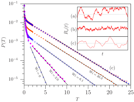
Figure 2: Linear-log plot of $P(T)$ versus $T$: the fitted $\alpha$’s for the four curves with $\mathrm{Wi}=0,2.0,6.1$, and $20.3$ are $1.20,0.57,0.375$, and $0.326$ respectively. The two datasets with symbols $\boxdot$ and $\blacktriangle$ in (c) are obtained by switching off the thermal noise along $x$ direction ($\eta_{1}=0$) in Eq. (1) and $\dot{\gamma}=0.2$ and $0.6$ respectively —both fit well with the analytical $\alpha=0.324$ line. All data are for $N=10$. Inset: Typical $R_{x}(t)$ versus $t$ corresponding to the cases (a) both $\dot{\gamma}\not=0$ and $\eta_{1}\not=0$, (b) $\dot{\gamma}=0$ and $\eta_{1}\not=0$, and (c) $\dot{\gamma}\not=0$ and $\eta_{1}=0$.

To check the accuracy of our analytical result Eq. (13), we perform a simulation switching off the thermal noise in the $x$ direction ($\eta_{1}=0$) in Eq. (1) —this effectively achieves the limit $\mathrm{Wi}\rightarrow\infty$ for any finite $\dot{\gamma}$. For the latter case, with $\dot{\gamma}=0.2$ and $0.6$, we show in Fig. 2 that their slopes $\alpha$ for $P(T)$ have excellent agreement with Eq. (13). For any finite $\mathrm{Wi}$ (keeping $\eta_{1}\not=0$), the value of $\alpha$ smoothly interpolates between the two limits $\simeq 1.20$ and $0.324$ (see Fig. 2).

No direct comparison can be made with the published experimental data gera , as the latter study is for radial tumbling. We look forward to future experiments on angular tumbling of a semi-flexible polymer. We claim that our result for $\alpha$ in Eq. (13) will serve as a lower bound, based on the following argument. For the small $\mathrm{Wi}$ regime, a semi-flexible polymer may be represented by the Rouse limit, for which we have shown (Fig. 2) that $\alpha$ decreases as $\mathrm{Wi}$ increases and approaches the value in Eq. (13) from above. On the other hand, for the large $\mathrm{Wi}$ regime, it is known from experiments gera and FENE model simulations celani that $\alpha$ increases as $\mathrm{Wi}$ increases. These two facts put together imply that $\alpha$ would reach a minimum value for some intermediate $\mathrm{Wi}$ and that can only approach the value in Eq. (13) from above. In summary, we have obtained exact PDFs for the length and latitude angle of the end-to-end vector of a Rouse polymer in shear flow. Further, we have derived an accurate analytical estimate of the decay constant associated with the PDF of angular tumbling times for a Rouse chain in the limit of strong shear.

References

• (1) P. G. De Gennes, J. Chem. Phys. 60, 5030 (1974).
• (2) D. E. Smith and S. Chu, Science 281, 1335 (1998).
• (3) P. LeDuc, C. Haber, G. Bao, and D. Wirtz, Nature 399, 564 (1999).
• (4) D. E. Smith, H. P. Babcock, and S. Chu, Science 283, 1724 (1999).
• (5) P. S. Doyle, B. Ladoux, and J. L. Viovy, Phys. Rev. Lett. 84, 4769 (2000).
• (6) A. Dua and B.J. Cherayil, J. Chem. Phys. 119, 5696 (2003).
• (7) M. Chertkov, I. Kolokolov, V. Lebedev, and K. Turitsyn, J. Fluid Mech. 531, 251 (2005).
• (8) A. Celani, A. Puliafito and K. Turitsyn, Europhys. Lett. 70, 464 (2005).
• (9) A. Puliafito and K. Turitsyn, Physica D 211, 9 (2005).
• (10) S. Gerashchenko and V. Steinberg, Phys. Rev. Lett. 96, 038304 (2006).
• (11) R. G. Winkler, Phy. Rev. Lett. 97, 128301 (2006).
• (12) S. Bhattacharya, D. Das, and S.N. Majumdar, Phys. Rev. E 75, 061122 (2007).
• (13) S. Chu, Phil. Trans. R. Soc. Lond. A 361, 689 (2003).
• (14) P.E. Rouse, J. Chem. Phys. 21, 1272 (1953).
• (15) J. Dubbeldam and F. Redig, J. Stat. Phys. 125, 225 (2006).
• (16) G. Wilemski and M. Fixman, J. Chem. Phys. 60, 866 (1974); 60, 878 (1974).
• (17) M. Doi, Chem. Phys. 9, 455 (1975); 11, 107 (1975); 11, 115 (1975).
• (18) A. E. Likthman and C. M. Marques, Europhys. Lett. 75, 971 (2006).
• (19) J. A. McFadden, IRE Trans. Inf. Theory 4, 14 (1957).
• (20) S. N. Majumdar, Curr. Sci. 77, 370 (1999).
• (21) S. N. Majumdar and C. Sire, Phys. Rev. Lett. 77, 1420 (1996).
• (22) S. N. Majumdar, C. Sire, A. J. Bray, and S. J. Cornell, Phys Rev. Lett. 77, 2867 (1996); B. Derrida, V. Hakim, and R. Zeitak, Phys. Rev. Lett. 77, 2871 (1996).
• (23) M. Doi and S.F. Edwards, The Theory of Polymer Dynamics (Oxford, New York, 1986).
• (24) I.S. Gradsteyn and I.M. Ryzhik, Tables of Inegrals, Series and Products (Academic Press, New York, 2000).
• (25) S.O. Rice, Bell Syst. Tech. J. 23, 282 (1944); 24, 46 (1945); [reprinted in Selected Papers on Noise and Stochastic Processes, edited by N. Wax (Dover, New York, 1954)].