Phase transitions in systems of magnetic dipoles on a square lattice with quenched disorder

Abstract

We study by Monte Carlo simulations the effect of quenched orientational disorder in systems of interacting classical dipoles on a square lattice. Each dipole can lie along any of two perpendicular axes that form an angle $\psi$ with the principal axes of the lattice. We choose $\psi$ at random and without bias from the interval $[-\Delta,\Delta]$ for each site of the lattice. For $0\leq\Delta\lesssim\pi/4$ we find a thermally driven second order transition between a paramagnetic and a dipolar antiferromagnetic order phase and critical exponents that change continously with $\Delta$. Near the case of maximum disorder $\Delta\approx\pi/4$ we still find a second order transition at a finite temperature $T_{c}$ but our results point to weak instead of strong long-ranged dipolar order for temperatures below $T_{c}$.

I Introduction

Systems of interacting dipoles (SIDs) are atracting a renewed interest. This is in part due to recent advances in nanoscience nano which render available realizations of magnetic nanoparticle assemblies array . These systems show a rich collective behaviour in which the dipole-dipole interactions play an essential role. This is because dipole-dipole interaction strength grows linearly with nanoparticle volume. Collective effects that are controlled by dipolar interactions can therefore become important at reasonably high temperatures. Spatial variations of the direction of magnetic dipolar fields lead to frustration and make SIDs very sensitive to their spatial arrangements our1 . In crystalline arrangements for example, SIDs exhibit different long ranged ferro or antiferromagnetic dipolar magnetic order that depends crucially on lattice geometry. The magnetic ordering depends also crucially in anisotropy. On the one hand, single site anisotropy is always present in magnetic crystals. On the other hand, dipole-dipole interactions by themselves create effective anisotropies in 2D systems. In square lattices, for example, dipole-dipole interactions pushes spins to lie on the plane of the lattice, and termal excitations tends to align them along the two principal axes of the lattice debell . The resulting magnetic order states that ensue from the competition of dipolar and anisotropic energies could be as exotic as ”spin ice” found in diamond type crystals ice . SIDs in disordered spatial arrangements are also of interest. Some non equilibrium spin glass behaviour (like time dependent susceptibilities and aging) has been observed in experiments with systems of randomly placed dipoles as frozen ferrofluids or strongly diluted magnetic crystals disorder . Very recent computer simulations indicate that systems of Ising dipoles with random anisotroy axes have an equilibrium spin glass phase at low temperaturesjul .

The aim of this paper is to study by numerical simulations the effect of quenched directional disorder in a system of dipoles placed in cristalline array. We are interested in how the magnetic dipolar order and the character of the transition between the paramagnetic and the low temperature ordered phase vary as we increase the amount of disorder. We also investigate whether there is a well defined threshold of disorder beyond which dipolar order dissapears.

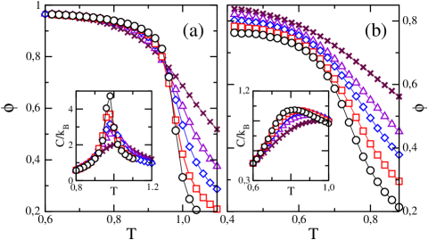
Figure 1: (a) Order parameter vs $T$ for systems with $\Delta=0.4$. $\times$, $\bigtriangleup$, $\diamond$, $\Box$ and $\circ$ stand for $L=8,12,26,22$ and $32$ respectively. Lines are only guides to the eyes. In the inset, specific heat vs. $T$ for the same $\Delta$ and systems sizes. (b) and inset therein, same as in (a) but for $\Delta=\pi/4$.

II Model and calculation

We first define the system model we use. Let ${\bf S}_{i}$ be a classical two xy-component unit spin at lattice site $i$ of a square lattice. These spins interact as pure magnetic dipoles with Hamiltonian

$$H=\sum_{\langle ij\rangle}\sum_{\alpha\beta}T_{ij}^{\alpha\beta}S_{i}^{\alpha}S_{j}^{\beta},$$ (1)

where

$$T_{ij}^{\alpha\beta}=\varepsilon_{d}\left(\frac{a}{r_{ij}}\right)^{3}\left(\delta_{\alpha\beta}-3\frac{r_{ij}^{\alpha}r_{ij}^{\beta}}{r_{ij}^{2}}\right),$$ (2)

${\bf r}_{ij}$ is the displacement from site $i$ to site $j$, $a$ is the square lattice parameter. In the following all energies and temperatures are given in terms of $\varepsilon_{d}$ and $\varepsilon_{d}/k_{B}$ respectively. When there is no quenched disorder, we consider a strong quadrupolar anisotropy that forces spins to lie along any of the two principal axis of the square lattice. This dipolar four-state clock model has been studied recently, and found to have a second order transition between a paramagnetic and an antiferromagnetic dipolar phase at $T_{c}=1.106$ with critical exponents $\alpha/\nu=0.82(5)$ and $\beta/\nu=0.03(2)$ our2 . In the ordered phase spins point up along lines with alternate sign from one line to the adjacent one. In order to characterize these antiferromagnetic order, we define a staggered magnetization as

$$(m_{x},m_{y})=N^{-1}(\sum_{i}S_{i}^{x}(-1)^{y(i)},\sum_{i}S_{i}^{y}(-1)^{x(i)}),$$ (3)

and use $\phi=(m_{x}^{2}+m_{y}^{2})^{1/2}$ as order parameter.

This system has been found to be very sensitive to the direction of the quadrupolar anisotropy axes. For example, if one turn these axes an angle $\psi=\pi/4$, critical exponents change to $\alpha/\nu=0.44(4)$ and $\beta/\nu=0.00(5)$unpub . Thus, we introduce disorder in the model described above by tilting these two orthogonal anisotropy axes by an angle $\psi$ with respect to the crystalline axes. For each spin this angle $\psi$ is chosen at random and without bias from the interval $[-\Delta,\Delta]$. Note that $\Delta=\pi/4$ correspond to a completely random distribution of the orientation of these pairs of axes. Note also that even in this case anisotropies never force any pair of spins to form angles greater that $\pi/4$. Therefore, this is less disruptive than random uniaxial anisotropy jul .

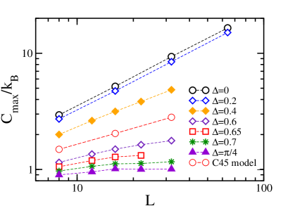
Figure 2: Log-log plot or the maximum value of the specific heat as a function of $L$ for the indicated values of $\Delta$. $\bullet$ stands for the model without disorder, but with quadrupolar easy axis forming angles of $pi/4$ with the $x,y$ axis at every site of the lattice.

We study systems of $L\times L$ spins and use periodic boundary conditions. We let a spin on site $i$ interact through dipolar fields with all spins within an $L\times L$ square centered on the $i$- site our2 . Our simulations follow the standard Metropolis Monte Carlo (MC) algorithm metrop . We use a single-spin flip dynamics, in which all dipolar fields are updated throughout the system every time a spin flip is accepted, before another spin is chosen in order to repeat the process. In our MC simulations, we start for a given realization of disorder from $T=2.5$ (well in the paramagnetic phase) and lower temperature in $\Delta T=0.05$ steps. At each value of $T$ we averaged over $5\times 10^{6}$ MC sweeps having first discarded $10^{6}$ MC sweeps to let the system equilibrate. Finally, our results are averaged over $N_{r}$ different independent realizations of quenched disorder. In order to get realiable results we use at least $N_{r}=200$ for $\Delta>0.6$ and $N_{r}=50$ for $\Delta<0.6$. As a result, error bars in the figures shown in this paper are always smaller than symbol sizes used therein. Our results follow from simulations for system sizes $L=8,12,16,22$ and $32$. This would be insuficient to obtain accurate critical exponent values but is adequate for our purposes.

We study the modulus of the staggered magnetization $\phi$ defined above and obtain the susceptibility from their fluctuations as $\chi=\delta\phi^{2}/(NT)$. We calculate the specific heat from energy fluctuations via the relation $C=\delta E^{2}/(NT^{2})$. Finally, we use the cumulant like quantity

$$u_{12}=[\pi/(4-\pi)][(4/\pi)-<\phi^{2}>/<\phi>^{2}]$$ (4)

As $L\to\infty$ we expect that $u_{12}\to 0$ in the paramagnetic phase, $u_{12}\to 1$ in the long ranged ordered phase and tend to some intermediate value at a critical point. Hence, curves of $u_{12}$ versus $T$ for different system sizes should cross at critical points for large enough $L$.

III Results

Data obtained for the order parameter $\phi$ for $\Delta=0.4$ are exhibited in a $\phi$ versus $T$ plot in figure 1(a). Curves for different $L$ cross at $T_{c}=0.95(1)$. Below this temperature $\phi$ increases as $L$ increases indicating the existence of an ordered phase. Plots for $\Delta=0.2,0.4,0.65$ and $0.7$ (not shown) are qualitalively similar, except in that curves for $L\geq 16$ tend to collapse below $T_{c}$ for the case $\Delta=0.7$. The behavior is markedly different for $\Delta\approx\pi/4$ (see Fig. 1(b)), where $\phi$ appears to decrease as $L$ increases even at low $T$ at least for the sizes we have studied, raising the question over the existence of strong long-range order. We return to this point in the discussion of Fig. 4.

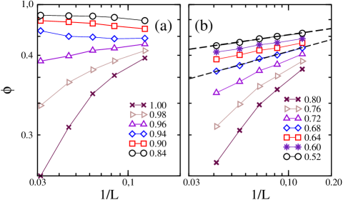
Figure 3: (a) Log-log plot of the order parameter versus $1/L$ for $\Delta=0.4$ and the temperatures indicated in the figure. Error bars are smaller than the size of the symbols. (b) Same as in (a) but for $\Delta=\pi/4$. Dashed thick lines in (b) stand for linear regression of the data. Thin solid lines are guides to the eyes.

In the inset of Fig. 1(a) we plot the specific heat $C$ vs $T$ for $\Delta=0.4$. Clearly a singularity develops as $L$ increases. We observe a weakening of this singularity as we increase $\Delta$ from $0$ to $0.7$. For $\Delta\approx\pi/4$ we see that the singularity washes out completely (see inset of Fig.  1(b)). In Fig.  2 we show a log-log plot of $C_{max}$ versus $T$, where $C_{max}$ is the value of the specific heat at its maximum. We obtain $\alpha/\nu$ from the straight line slopes using $C_{max}\propto L^{\alpha/\nu}$. This is so for $\Delta=0.2,0.4$ and $0.6$ for which we obtain $\alpha/\nu=0.83(4),0.63(4)$ and and $0.31(6)$ respectively. In contrast, data plotted in Fig. 2 for $\Delta>0.6$ show not straight lines but curves that become flatter as $L$ increases suggesting that $\alpha/\nu=0$. This dependence of $\alpha/\nu$ with $\Delta$ is in agreement with the Harris criterion harris , in principle valid only for systems with short ranged interactions.

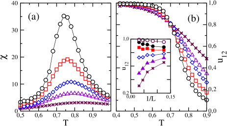
Figure 4: (a) Susceptibility versus $T$ for $\Delta=\pi/4$. $\times$, $\bigtriangleup$, $\diamond$, $\Box$ and $\circ$ stand for $L=8,12,26,22$ and $32$ respectively Lines are only guides to the eyes. (b) Cumulant $u_{12}$ versus $T$ for $\Delta=\pi/4$. Symbols stand for the same system sizes as in (a). In the inset of Fig. (b), $u_{12}$ versus $1/L$ for different temperatures and $\Delta=\pi/4$. $\circ$, $\bullet$, $\blacksquare$, $\diamond$, $\blacktriangle$ and $\times$ stand for $T=0.80,0.76,0.72,0.68,0.64$ and $0.52$ respectively.

We next discuss whether strong or weak long-range order exists at low temperatures for $\Delta=\pi/4$. For this purpose, we compare log-log plots of $\phi$ vs $1/L$ for $\Delta=0.6$ and $\Delta=\pi/4$. These plots are shown in Figs. 3(a) and 3(b) respectively and are qualitalively different. Fig. 3(a) is consistent with a phase transition from a magnetically disorder state above $T=0.95(1)$ to a strong long range order below them. We have obtained similar behaviour for other values of $\Delta$ in the $(0,0.7)$ range. On the other hand, in Fig. 3(b) $\phi$ appears to decrease algebraically with $L$ over a wide range of temperatures for $T\leq 0.68$ Dashed thick lines in the figure stand for linear regression of the data for $T=0.52$ and $0.68$ and their slope gives $\beta/\nu=0.06(2)$ and $0.12(4)$ respectively using $\phi\propto L^{\beta/\nu}$.

We also gathered information from the behaviour of susceptibility $\chi$. In Fig. 4(a), plots of $\chi$ vs $T$ for $\Delta=\pi/4$ show curves whose peak grows as $L$ increases. From the data shown, we obtain $\chi_{max}\propto L^{1.85(5)}$ where $\chi_{max}$ stands for the maximum value of $\chi$ versus $T$ for a given value of $L$. We obtain qualitatively similar results for $\Delta<\pi/4$. Note also in Fig. 4(a) that the position of the maximum of $\chi$, $T_{m}$, changes with $L$. In the inset of Fig. 5 we plot $T_{m}$ versus $1/L$ for different values of $\Delta$. Direct extrapolation of these data to $1/L\to 0$ gives an estimation of the transition temperature $T_{c}$. The resulting values of $T_{c}$ vs $\Delta$ are plotted in Fig. 5.

A more accurate determination of $T_{c}$ and some additional information about the nature of the transition was obtained from $u_{12}$. In Fig. 4(a) we plot $u_{12}$ vs $T$ for $\Delta=\pi/4$. Curves for different values of $L$ exhibit a clear crossing at $T_{c}=0.69(1)$ and $u_{12}=0.82(1)$. We have obtained similar plots for various values of $\Delta$ that enabled us to estimate $T_{c}$ by the value of $T$ where the curves cross. The resulting values of $T_{c}$ are plotted vs $\Delta$ in Fig. 5, which gives the global phase diagram for our model. In the inset of Fig. 4(b) we plot $u_{12}$ versus $1/L$ for $\Delta=\pi/2$. For the system sizes we have considered, curves exhibit marked finite size effects even well below $T=0.69$. Results for $T=0.52$ and $0.64$ shown in this inset seem to indicate that $u_{12}\to 1$ as $1/L\to 0$ or at least that $1\leq<\phi^{2}>/<\phi>^{2}<1.02$. This is consistent with the behaviour koster found for $u_{12}$ for 2D $XY-like$ models that exhibit a Kosterlitz-Thouless transition with weak long-range order below a transition temperature.

In sum, we have reported evidence from MC simulations that disorder in the orientation of the quadrupolar anisotropy axes on systems of interacting dipoles in square lattice is relevant, in the sense that modifies the critical behavior of the thermal transition between a paramagnetic and the antiferromagnetic dipolar phase.

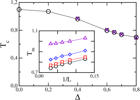
Figure 5: Transition temperature $T_{c}$ versus $\Delta$. $\bigcirc$ stand for values of $T_{c}$ obtained from extrapolation of temperatures at which susceptibility attains its maximum for different values of $L$ (see text). $\times$ stand for $T_{c}$ obtained as the temperature for which $u_{12}$ is independent of $L$. In the inset, temperature of maximum susceptibility versus $1/L$. $\triangle$, $\diamond$, $\square$ and $\circ$ stand for $\Delta=0.4,0.6,0.7$ and $\pi/2$ respectively.

We enjoyed interesting discussions with J. F. Fernández and are grateful to Institute Carlos I at University of Granada for much computer time. We thank financial support from Grant FIS2006-00708 from the Ministerio de Ciencia e Innovación of Spain.

References

- (1) i R. P. Cowburn, Philos. Trans. R. Soc. London, Ser. A 358, 281 (2000); R. J. Hicken, ibid. 361, 2827 (2003).
- (2) R. F. Wang et al., Nature (London) 439, 303 (2006).
- (3) J. Luttinger and L. Tisza, Phys. Rev. 72, 257 (1947); J. J. Alonso and J. F. Fernández, Phys. Rev. B 62, 53 (2000).
- (4) K. De’Bell, A. B. MacIsaac, I. N. Booth, and J. P. Whitehead, Phys. Rev. B 55, 15108 (1997); J. F. Fernández and J. J. Alonso, Phys. Rev. B 74, 184416 (2006)
- (5) A. P. Ramirez, A. Hayashi ,A. Cava, R. J. Siddharthan, and B. S. Shastry, Nature (London) 399, 333 (1999); S. T. Bramwell and M. P. J. Gingras, Science 294, 1495 (2001).
- (6) W. Luo, S. R. Nagel, T. F. Rosenbaum, and R. E. Rosensweig, Phys. Rev. Lett. 67, 2721 (1991); T. Jonsson, J. Mattsson, C. Djurberg, F. A. Khan, P. Nordblad, and P. Svedlindh, Phys. Rev. Lett. 75, 4138 (1995); S. Ghosh, R. Parthasarathy, T. F. Rosenbaum, and G. Aeppli, Science 296, 2195 (2002).
- (7) J. F. Fernández, accepted for publication in Phys. Rev. B.
- (8) J. F. Fernández and J. J. Alonso, Phys. Rev. B 76, 014403 (2007).
- (9) (unpublished work).
- (10) N. A. Metropolis, A. W. Rosenbluth, M. N. Rosenbluth, A. H. Teller, and E. Teller, J. Chem. Phys. 21, 1087 (1953).
- (11) A. B. Harris, J. Phys. C 7, 1671 (1974).
- (12) L. A. S. Mól, A. R. Pereira, H. Chamati, and S. Romano, Eur. Phys. J. B 50, 541 (2006).