Explicit tensor network representation for the ground states of string-net models

Abstract

The structure of string-net lattice models, relevant as examples of topological phases, leads to a remarkably simple way of expressing their ground states as a tensor network constructed from the basic data of the underlying tensor categories. The construction highlights the importance of the fat lattice to understand these models.

I Introduction

Topological phases of lattice models recently attracted interest because of their potential use as quantum memories and quantum computers Kitaev . While it is unclear whether their shortcomings at finite temperature can be satisfactorily resolved finiteT , these models remain appealing as systems with topological order WenOrder and quantum error correcting codes. The first such proposal was Kitaev’s paper Kitaev , where the Abelian toric code was introduced, and a class of non-Abelian generalisations, the quantum double models, with roots in the theory of Hopf algebras. These are examples of gauge models with discrete gauge group Wegner ; Bais . More recently, Levin and Wen LevinWen introduced their string-net models, arguing for string-net condensation as a basic mechanism underlying topological order. A crucial device in the formulation of these models is the fat lattice, which allows an interpretation of the lattice model in terms of a theory in the continuum, and provides insight in the role of the operators constituting the Hamiltonian.

In order to have a handle on the properties of topological phases on the lattice, it is desirable to have as much theoretical control as possible over the form of topological states. Accordingly, explicit tensor network representations for the ground state of string-net models have been recently presented. Thus, Ref. VerstraetePower describes a projected entangled-pair state (PEPS) representation of the toric code and resonating valence bond states, whereas a multi-scale entanglement renormalization ansatz (MERA) representation of all quantum doubles AguadoVidal and all string-net models Koenig is also known. Finally, Ref.  GuTopo discusses a double line tensor network representation of the $\mathbb{Z}_{2}$ gauge model and the double-semion model.

In this work we describe a simple construction expressing the ground states of any string-net model as a tensor network constructed with $F$-tensors. The starting point is the form of the Hamiltonian as a sum of commuting projectors, $H=-\sum_{i}P_{i}$, which leads to the realisation of the ground level as the $+1$ eigenspace of the product $\prod_{i}P_{i}$. The tensor network follows in a remarkably straightforward way. Its form is reminiscent of a classical statistical mechanical partition function with local (albeit possibly complex) weights, which is why we call it a Boltzmann weight tensor network. The needed ingredients are the data of the underlying tensor category as explained in LevinWen , i. e., the fusion rules and associated $F$-tensors. The construction is most appropriately understood from the fat lattice perspective.

In section II, we provide a short exposition to string-net models and the fat lattice picture. In section III, the Boltzmann weight tensor network construction for string-net ground states is presented step by step. Essentially, we use the projectors on the ground level in order to build a simple expression for the ground state using $F$-tensors.

The Boltzmann weight tensor network differs from the MERA of Ref. Koenig , also written in terms of $F$-tensors, in that it is much simpler than the latter—e. g., it is a two-dimensional network, while the MERA spans three dimensions. On the other hand, although conceived independently, our construction coincides for the $\mathbb{Z}_{2}$ gauge and double-semion models with the double line tensor network of Ref. GuTopo , where the authors also hint at an unpublished result for generic string-net models.

II String-nets and the fat lattice

String-net models were introduced in LevinWen in order to encode the universal physical properties of doubled $(2+1)D$ topological phases of matter in quantum lattice models with few-body interactions. The simple structure of their Hamiltonians reflects their conception as infrared fixed points of renormalization group flows. Explicitly, these Hamiltonians are exactly solvable because they are given by the sum of mutually commuting terms. In the following, we consider those models in LevinWen which exhibit a well-defined continuum limit.

These models are defined on a hexagonal lattice $\Lambda$. Local degrees of freedom are associated with oriented edges of $\Lambda$ and elements of the computational basis are labelled by $i\in\{1,\dots,N\}$. These labels may be interpreted as particle species propagating along the edges. For each label $i$ there is a unique label $i^{*}$ denoting its antiparticle, and reversing the orientation of an edge corresponds to the mapping $i\mapsto i^{*}$. The label $1$ stands for the absence of any particle (vacuum). Furthermore, each instance of a string-net model is equipped with a set of fusion rules $\delta_{ijk}$ specifying allowed ($\delta_{ijk}=1$) and forbidden ($\delta_{ijk}=0$) configurations of labels incident to a vertex. Given the set of labels and their fusion rules, one can build a tensor category which includes recoupling relations encapsulated in the symbol $F_{kln}^{ijm}$ (akin to the $6j$-symbol in the theory of angular momentum), and an assignment of quantum dimensions $d_{i}$ to the labels. The total quantum dimension is given by $\mathcal{D}=\bigl{(}\sum_{i=1}^{N}d_{i}^{2}\bigr{)}^{1/2}$.

Fixed-point wavefunctions are constructed from local constraints LevinWen which are crafted so as to enforce topological invariance of the wavefunction. These local constraints are assembled from the objects $d_{i}$, $F_{kln}^{ijm}$ introduced above. Furthermore there is a natural correspondence between physical configurations on $\Lambda$ and configurations of string-nets in the fat lattice. The latter is constructed from the physical lattice $\Lambda$ by puncturing the underlying surface at the center of each plaquette. String-nets consist of oriented strings carrying labels in the set $\{1,\dots,N\}$, joined at trivalent branching points in a way that respects the fusion rules $\delta_{ijk}$, and avoiding the punctures. String-net configurations are defined to be equivalent if they can be transformed into each other using the local relations (smooth deformations avoiding punctures, recoupling by $F$-symbols, trading isolated loops for quantum dimensions, and label conservation). Equivalence classes are identified with physical configurations. Note that the physical configuration itself can be regarded as a particular string-net identical with the physical lattice. We will refer to this particular string-net as the canonical representative of the equivalence class, and its uniqueness is ensured by Mac Lane’s coherence theorem MacLane .

The Hamiltonian on the physical lattice reads

$$H=-\sum_{v}A_{v}-\sum_{p}B_{p},$$

where the sums range over the vertices and plaquettes of the lattice. Vertex terms are projectors enforcing the fusion rules

$$A_{v}=\sum_{i,j,k\in v}\delta_{ijk}\,\lvert ijk\rangle\langle ijk\rvert$$

while plaquette projectors represent the kinetic part of the Hamiltonian and are defined by

$$B_{p}=\sum_{\alpha_{p}=1}^{N}\frac{d_{\alpha_{p}}}{\mathcal{D}^{2}}B_{p}^{\alpha_{p}},$$

where $B_{p}^{\alpha_{p}}$ acts on the plaquette $p$ together with the outer legs of $p$. Its precise definition is given in LevinWen , as well as the following simple graphical interpretation on the fat lattice: $B_{p}^{\alpha_{p}}$ creates an isolated loop of label $\alpha_{p}$ around the puncture at plaquette $p$.

III Ground states of string-net models as tensor networks

Let $\Lambda^{*}$ denote the dual lattice of $\Lambda$. It is instructive to decompose the edge set of $\Lambda^{*}$ as

$$E(\Lambda^{*})=\bigcup_{i=1}^{3}E_{i}$$ (1)

where $E_{1}$ denotes the set of horizontal edges, $E_{2}$ one set of parallel diagonal edges, and $E_{3}$ the other one as can be seen from Fig. 1.

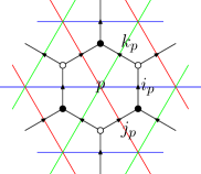
Figure 1: Hexagonal lattice $\Lambda$ and its dual $\Lambda^{*}$. Horizontal edges (blue) of $\Lambda^{*}$ belong to $E_{1}$, diagonal edges (red) to $E_{2}$ and diagonal edges (green) to $E_{3}$. The directed edges of $\Lambda$ are labelled by uniquely associating them to a face. Circled vertices of $\Lambda$ belong to the even sublattice $\Lambda_{1}$, filled ones to the odd sublattice $\Lambda_{2}$.

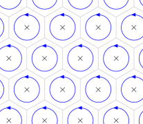
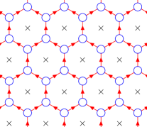
$\mapsto$ $\mapsto$

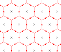
Figure 2: Reducing the fat lattice. In (a) an isolated loop at face $p$ carries a label $\alpha_{p}$ and all edges $E(\Lambda)$ (grey) of the physical lattice are labelled by $0$. The overall quantum state is denoted by $\lvert\{\alpha_{p}\}\rangle$. Three rounds of $F$-moves reduce to the fat lattice configuration (b) which carries both the final physical labels $i_{p}$, $j_{p}$, $k_{p}$ as well as the labels $\alpha_{p}$ at the vertex loops. This is denoted by $\lvert\{\alpha_{p},i_{p},j_{p},k_{p}\}\rangle$. In (c) each vertex has been fully reduced to the physical lattice by a sequence of another two $F$-moves each. The corresponding physical quantum state is given by $\lvert\{i_{p},j_{p},k_{p}\}\rangle$.

In order to construct an explicit graphical expression for a ground state of a string-net model, we start with the state $\lvert 1\dots 1\rangle$ on the physical lattice where all edges carry the vacuum label $1$. Note that this can be represented by a completely empty fat lattice. Obviously, this state is an eigenstate of all the $A_{v}$ operators with eigenvalue $+1$. Since the Hamiltonian is frustration-free we end up in the ground level by applying the projection $\prod_{p}B_{p}$.

Thus, up to an overall factor, this ground state on the physical lattice is represented by the following string-net state on the fat lattice:

$$\lvert\Psi_{0}\rangle=\biggl{(}\prod_{p}d_{\alpha_{p}}\biggr{)}\,\lvert\{\alpha_{p}\}\rangle$$ (2)

where $\lvert\{\alpha_{p}\}\rangle$ denotes the string-net configuration shown in Fig. 2(a).

From now on we will use the local relations of the string-net model in order to reduce Eq. (2) to its canonical representative, which can be directly translated into a configuration on the physical lattice.

After applying three rounds of recouplings involving $F$-symbols ($F$-moves) to the strings on the fat lattice one has:

$$\lvert\Psi_{0}\rangle = \sum_{\{\alpha_{p}\}}\biggl{(}\prod_{p}d_{\alpha_{p}}\biggr{)}\!\sum_{\{i_{p},j_{p},k_{p}\}}\!\biggl{(}\,\prod_{(p,q)\in E_{1}}\!F_{\alpha_{q}^{*}\alpha_{q}i_{p}}^{\alpha_{p}^{*}\alpha_{p}0}\biggr{)}$$ (3)

$${}\times\biggl{(}\,\prod_{(p,q)\in E_{2}}\!F_{\alpha_{q}^{*}\alpha_{q}j_{p}}^{\alpha_{p}^{*}\alpha_{p}0}\biggr{)}\biggl{(}\,\prod_{(p,q)\in E_{3}}\!F_{\alpha_{q}^{*}\alpha_{q}k_{p}}^{\alpha_{p}^{*}\alpha_{p}0}\biggr{)}$$

$${}\times\,\lvert\{\alpha_{p},i_{p},j_{p},k_{p}\}\rangle,$$

where $\lvert\{\alpha_{p},i_{p},j_{p},k_{p}\}\rangle$ denotes the state of the fat lattice as shown in Fig. 2(b). Using the normalization

$$F_{j^{*}jk}^{ii^{*}0}=\sqrt{\frac{d_{k}}{d_{i}d_{j}}}\,\delta_{ijk}$$ (4)

this expression can be simplified in the case of an infinite or periodic lattice to yield:

$$\lvert\Psi_{0}\rangle=\!\sum_{\{\alpha_{p},i_{p},j_{p},k_{p}\}_{\star}}\!\biggl{(}\prod_{p}\frac{\sqrt{d_{i_{p}}d_{j_{p}}d_{k_{p}}}}{d_{\alpha_{p}}^{2}}\biggr{)}\,\lvert\{\alpha_{p},i_{p},j_{p},k_{p}\}\rangle.$$ (5)

Note that we have omitted the $\delta$-symbols and rather restricted the sum to configurations $\{\alpha_{p},i_{p},j_{p},k_{p}\}_{\star}$ that respect the branching rules of the particular string-net model.

For a full reduction to the physical lattice we eventually need to remove the loops at the vertices. This can be done by applying two $F$-moves at each vertex:

$$\lvert\{\alpha_{p},i_{p},j_{p},k_{p}\}\rangle = \biggl{(}\prod_{p}\frac{d_{\alpha_{p}}^{2}}{\sqrt{d_{i_{p}}d_{k_{p}}}}\biggr{)}\prod_{v\in\Lambda_{1}}f(v)$$ (6)

$${}\times\!\prod_{v^{\prime}\in\Lambda_{2}}\!g(v^{\prime})\,\lvert\{i_{p},j_{p},k_{p}\}\rangle$$

Here $\Lambda_{i}$ denote the even and odd sublattices of $\Lambda$ respectively and furthermore one has:

$$f(v) = F_{k_{r}\alpha_{q}i_{p}}^{\alpha_{p}^{*}j_{p}\alpha_{r}}$$ (7)

$$g(v^{\prime}) = F_{j_{q}^{*}\alpha_{q}k_{p}}^{\alpha_{p}^{*}i_{p}\alpha_{r}}$$ (8)

where the faces $\{p,q,r\}$ of $\Lambda$ surround an even vertex $v$ or an odd vertex $v^{\prime}$ as indicated in Fig. 3.

Figure 3: Even (circled) and odd (filled) vertices of $\Lambda$ with their surrounding faces.

At this point the ground state of the string-net model can be written in terms of the physical lattice only:

$$\lvert\Psi_{0}\rangle = \!\sum_{\{\alpha_{p},i_{p},j_{p},k_{p}\}}\!\biggl{(}\prod_{p}\sqrt{d_{j_{p}}}\biggr{)}\prod_{v\in\Lambda_{1}}f(v)\prod_{v^{\prime}\in\Lambda_{2}}g(v^{\prime})$$ (9)

$${}\times\,\lvert\{i_{p},j_{p},k_{p}\}\rangle.$$

Note that because of the convention for the $F$-symbols in LevinWen the branching rules at each vertex are automatically satisfied and we no longer need to restrict the sum. This allows one to isolate the basis coefficients:

$$\lambda_{\{i_{p},j_{p},k_{p}\}}=\biggl{(}\prod_{p}\sqrt{d_{j_{p}}}\biggr{)}\sum_{\{\alpha_{p}\}}\prod_{v\in\Lambda_{1}}f(v)\prod_{v^{\prime}\in\Lambda_{2}}g(v^{\prime}).$$ (10)

It is this very expression that we are now going to write in a graphical fashion as a contracted tensor network.

In order to write the coefficients of the string-net model ground state given by Eq. (10) in a graphical fashion it is instructive to proceed locally. Let us therefore consider an arbitrary face $a$ of $\Lambda$ together with its next neighbours $b,\dots,g$. Obviously, the sum over $\alpha_{a}$ can now be carried out immediately and will involve no more than six $F$-symbols. Thus we obtain the following local expression:

$$\lambda_{\{i_{p},j_{p},k_{p}\}} \sim \sqrt{d_{j_{a}}d_{j_{d}}}\,\sum_{\alpha_{a}}F_{k_{g}\alpha_{b}i_{a}}^{\alpha_{a}^{*}j_{a}\alpha_{g}}\,F_{k_{a}\alpha_{c}i_{d}}^{\alpha_{d}^{*}j_{d}\alpha_{a}}\,F_{k_{f}\alpha_{a}i_{e}}^{\alpha_{e}^{*}j_{e}\alpha_{f}}$$ (11)

$${}\times F_{j_{c}^{*}\alpha_{c}k_{a}}^{\alpha_{a}^{*}i_{a}\alpha_{b}}\,F_{j_{d}^{*}\alpha_{d}k_{e}}^{\alpha_{e}^{*}i_{e}\alpha_{a}}\,F_{j_{a}^{*}\alpha_{a}k_{f}}^{\alpha_{f}^{*}i_{f}\alpha_{g}}.$$

Now define two sets of vertex tensors for the even and odd sublattices of $\Lambda$ by

$$:= T_{\mu\mu^{\prime}\nu\nu^{\prime}\lambda\lambda^{\prime}}^{[ijk]}$$ (12)

$$:= \tilde{T}_{\mu\mu^{\prime}\nu\nu^{\prime}\lambda\lambda^{\prime}}^{[ijk]}$$ (13)

where

$$T_{\mu\mu^{\prime}\nu\nu^{\prime}\lambda\lambda^{\prime}}^{[ijk]} := \sqrt{d_{j}}\,F_{k\mu i}^{\nu^{*}\!j\lambda}\,\delta_{\mu\mu^{\prime}}\delta_{\nu\nu^{\prime}}\delta_{\lambda\lambda^{\prime}}$$ (14)

$$\tilde{T}_{\mu\mu^{\prime}\nu\nu^{\prime}\lambda\lambda^{\prime}}^{[ijk]} := F_{j^{*}\lambda k}^{\mu^{*}i\nu}\,\delta_{\mu\mu^{\prime}}\delta_{\nu\nu^{\prime}}\delta_{\lambda\lambda^{\prime}}$$ (15)

and contract them according to the network given in Fig. 4(a). If we cut out a single face of this network it can easily be verified that it exactly reproduces the local form of our coefficients as in Eq. (11), up to the factor $\sqrt{d_{j_{e}}}$ (which can be absorbed, as the summation is extended to the adjacent faces).

Thus we have obtained a simple graphical notation that describes the ground state of an arbitrary string-net model and involves local terms only. In fact, following the arguments of LevinWen , our graphical calculus encompasses the ground states of all “doubled” topological phases in the infrared limit.

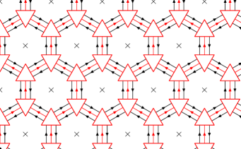
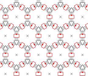
Figure 4: (a) Tensor network describing the ground state of an arbitrary string-net model. In this figure only virtual bonds (black) are summed over while physical indices (red) are left uncontracted. (b) Tensor network describing the ground state of an arbitrary string-net model. In this figure all bonds are contracted.

We can also pull out the indices from the vertex tensors and collect physical indices that denote particle and antiparticle into a single physical index at the edge. This can be done by defining the following tensors:

$$\vbox{\hbox{\includegraphics{tensors-2.pdf}}}\!=A_{\alpha\alpha^{\prime}\mu\mu^{\prime}\nu\nu^{\prime}}^{[i]}$$ (16)

$$= B_{\alpha\beta\gamma\mu\mu^{\prime}\nu\nu^{\prime}\lambda\lambda^{\prime}}$$ (17)

$$= \tilde{B}_{\alpha\beta\gamma\mu\mu^{\prime}\nu\nu^{\prime}\lambda\lambda^{\prime}}$$ (18)

where

$$A_{\alpha\alpha^{\prime}\mu\mu^{\prime}\nu\nu^{\prime}}^{[i]} := \delta_{i\alpha}\delta_{\alpha\alpha^{\prime}}\delta_{\mu\mu^{\prime}}\delta_{\nu\nu^{\prime}}$$ (19)

$$B_{\alpha\beta\gamma\mu\mu^{\prime}\nu\nu^{\prime}\lambda\lambda^{\prime}} := T_{\mu\mu^{\prime}\nu\nu^{\prime}\lambda\lambda^{\prime}}^{[\alpha\beta\gamma]}$$ (20)

$$\tilde{B}_{\alpha\beta\gamma\mu\mu^{\prime}\nu\nu^{\prime}\lambda\lambda^{\prime}} := \tilde{T}_{\mu\mu^{\prime}\nu\nu^{\prime}\lambda\lambda^{\prime}}^{[\alpha\beta\gamma]}$$ (21)

and contracting them according to Fig. 4(b). Note that the vertex tensors $T$ and $B$ only differ in how their indices are regarded: what used to be a physical index of $T$ has been changed into a virtual one of $B$. Thus the vertex tensors $B$ and $\tilde{B}$ are contracted on the virtual level exclusively.

IV Conclusions and outlook

In this paper we have derived a remarkably simple tensor network representation for Levin and Wen’s string-net ground states. This construction follows directly from the characterisation of these states as simultaneous $+1$ eigenstates of the projectors in the Hamiltonian. It also heavily relies on the notion of the fat lattice. Understanding string-net models in terms of the mapping from the fat lattice to the physical lattice thus leads to insight and useful results. The tensor network is built from the fusion rules and $F$-tensors of the tensor category underlying the string-net model.

Note that from our Boltzmann weight tensor network one can trivially build a PEPS representation. In the case of quantum double models, which can be explicitly written as string-net models, dramatic simplifications to this PEPS representation are possible due to their group-theoretical properties. Also, for a general string-net model it is possible to express excited states by absorbing their corresponding open string operators into a ground state tensor network representation. These topics will be discussed in QDSN .

Due to its simplicity (as compared to the full-fledged specification of all stabilizer operators) this tensor network representation will help study a range of properties of the ground level sector. For example, the topological entanglement entropy TEE is one such property hinting at the presence of a new kind of multipartite, long-range entanglement that appears to underlie topological order. Along the same lines it may be interesting to establish criteria for a tensor network to represent a ground state of some topologically ordered quantum system. Of course, for this it would be necessary to extend the present analysis beyond the infrared limit as given by the string-net models.

- (1) A. Kitaev, Annals Phys. 303, 2 (2003), arXiv: quant-ph/9707021.
- (2) C. Castelnovo and C. Chamon, Phys. Rev. B 76, 184442 (2007); Z. Nussinov and G. Ortiz, arXiv:cond-mat/0702377; S. Iblisdir et al., arXiv:0806.1853; A. Kay, arXiv:0807.0287.
- (3) X.-G. Wen, Adv. Phys. 44, 405 (1995), arXiv: cond-mat/9506066.
- (4) F. J. Wegner, J. Math. Phys. 12, 2259 (1971).
- (5) M. De Wild Propitius, F. A. Bais, arXiv: hep-th/9511201.
- (6) M. A. Levin, X.-G. Wen, Phys. Rev. B71, 045110 (2005), arXiv:cond-mat/0404617.
- (7) F. Verstraete, M. M. Wolf, D. Pérez-García, and J. I. Cirac, Phys. Rev. Lett. 96, 220601 (2006), arXiv: quant-ph/0601075
- (8) M. Aguado and G. Vidal, Phys. Rev. Lett. 100, 070404 (2008), arXiv:0712.0348.
- (9) R. Koenig, B. W. Reichardt, G. Vidal, arXiv:0806.4583.
- (10) Zh.-Ch. Gu, M. Levin and X.-G. Wen, arXiv:0807.2010.
- (11) S. Mac Lane, Categories for the working mathematician, 2nd Ed., Springer (1998).
- (12) O. Buerschaper et al., in preparation.
- (13) A. Hamma, R. Ionicioiu, P. Zanardi, Phys. Lett. A 337, 22 (2005), arXiv:quant-ph/0409073; M. Levin, X.-G. Wen, Phys. Rev. Lett. 96, 110405 (2006), arXiv:cond-mat/0510613; A. Kitaev, J. Preskill, Phys. Rev. Lett. 96, 110404 (2006), arXiv:quant-ph/0510231.