How To Determine SUSY Mass Scales Now

Abstract

Currently available experimental data from electroweak precision observables (EWPO), $B$-physics observables (BPO) and cosmological data can be combined to extract the preferred value of SUSY mass scales. We review recent results on the predictions of the masses of supersymmetric particles and the indirect determination of the lightest Higgs boson mass. Special emphasis is put on models going beyond the Constrained Minimal Supersymmetric Standard Model (CMSSM), such as the Non-Universal Higgs Model type I (NUHM1), or gauge and anomaloy mediated SUSY breaking.

1 INTRODUCTION

The Standard Model (SM) cannot be the ultimate theory of particle physics. While describing direct experimental data reasonably well, it fails to include gravity, it does not provide cold dark matter, and it has no solution to the hierarchy problem, i.e. it does not have an explanation for a Higgs-boson mass at the electroweak scale.

Theories based on Supersymmetry (SUSY) mssm are widely considered as the theoretically most appealing extension of the SM. They are consistent with the approximate unification of the gauge coupling constants at the GUT scale and provide a way to cancel the quadratic divergences in the Higgs sector hence stabilizing the huge hierarchy between the GUT and the Fermi scales. Furthermore, in SUSY theories the breaking of the electroweak symmetry is naturally induced at the Fermi scale, and the lightest supersymmetric particle can be neutral, weakly interacting and absolutely stable, providing therefore a natural solution for the dark matter problem. SUSY predicts the existence of scalar partners $\tilde{f}_{L},\tilde{f}_{R}$ to each SM chiral fermion, and spin–1/2 partners to the gauge bosons and to the scalar Higgs bosons. The Higgs sector of the Minimal Supersymmetric Standard Model (MSSM) with two scalar doublets accommodates five physical Higgs bosons. In lowest order these are the light and heavy ${\cal CP}$-even $h$ and $H$, the ${\cal CP}$-odd $A$, and the charged Higgs bosons $H^{\pm}$. So far, the direct search for SUSY particles has not been successful. One can only set lower bounds of ${\cal O}(100)$ GeV on their masses pdg .

Besides the direct detection of SUSY particles (and Higgs bosons), physics beyond the SM can also be probed by precision observables via the virtual effects of the additional particles. Observables (such as particle masses, mixing angles, asymmetries etc.) that can be predicted within the MSSM and thus depend sensitively on the model parameters constitute a test of the model on the quantum level. The most relevant electroweak precision observables (EWPO) in this context are the $W$ boson mass, $M_{W}$, the effective leptonic weak mixing angle, $\sin^{2}\theta_{\mathrm{eff}}$, and the anomalous magnetic moment of the muon, $a_{\mu}\equiv(g-2)_{\mu}/2$. Since the lightest MSSM Higgs boson mass, $M_{h}$ can be predicted, it also constitutes a precision observable. An overview of SUSY effects on EWPO can be found in Ref. PomssmRep .

An example how the EWPO can restrict the SM or the MSSM parameter space is shown in Fig. 1 FeynW ; FeynZ . The plot compares the the combined prediction for $M_{W}$ and $\sin^{2}\theta_{\mathrm{eff}}$ in the SM and the MSSM. The predictions within the two models give rise to two bands in the $M_{W}$–$\sin^{2}\theta_{\mathrm{eff}}$ plane with only a relatively small overlap sliver (indicated by a dark-shaded (blue) area in Fig. 1). The allowed parameter region in the SM (the medium-shaded (red) and dark-shaded (blue) bands) arises from varying two parameters: the mass of the SM Higgs boson, from $M_{H}^{\mathrm{SM}}=114\,\,\mathrm{GeV}$, the LEP exclusion bound LEPHiggsSM to $400\,\,\mathrm{GeV}$ as indicated by an arrow; the other parameter is the top quark mass, which has been varied from $165\,\,\mathrm{GeV}$ to $175\,\,\mathrm{GeV}$, which is also indicated by an arrow, where the current experimental value is $m_{t}^{\rm exp}=172.4\pm 1.2\,\,\mathrm{GeV}$ mt1724 , The light shaded (green) and the dark-shaded (blue) areas indicate allowed regions for the unconstrained MSSM, obtained from scattering the relevant parameters independently FeynZ . The decoupling limit with SUSY masses of ${\cal O}(2\,\,\mathrm{TeV})$ yields the upper edge of the dark-shaded (blue) area. Thus, the overlap region between the predictions of the two models corresponds in the SM to the region where the Higgs boson is light, i.e. in the MSSM allowed region ($M_{h}\;\raisebox{-3.00003pt}{$\stackrel{{\scriptstyle\displaystyle<}}{{\sim}}$}\;135\,\,\mathrm{GeV}$ mhiggslong ; mhiggsAEC ). In the MSSM it corresponds to the case where all superpartners are heavy, i.e. the decoupling region of the MSSM. The current experimental limits LEPEWWG ; TEVEWWG ,

$$M_{W}^{\rm exp} =80.399\pm 0.025\,\,\mathrm{GeV}~{},$$ (1)

$$\sin^{2}\theta_{\mathrm{eff}}^{\rm exp} =0.23153\pm 0.00016$$ (2)

are indicated in the plot. As can be seen from Fig. 1, the current experimental 68% C.L. region for $M_{W}$ and $\sin^{2}\theta_{\mathrm{eff}}$ exhibits a slight preference of the MSSM over the SM.

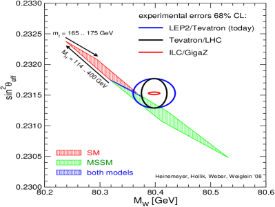
\begin{picture}(0.0,0.0) \put(0.0,0.0){} \put(0.0,0.0){} \end{picture}

Figure 1: Prediction for $M_{W}$ and $\sin^{2}\theta_{\mathrm{eff}}$ in the MSSM and the SM (see text) FeynZ . Also shown are the present experimental results for $M_{W}$ and $\sin^{2}\theta_{\mathrm{eff}}$ at the 68% C.L.

Other important ingredients for the determination of SUSY mass scales from current experimental data are $B$-physics observables (BPO), see e.g. Refs. LSPlargeTB ; hfag and the abundance of cold dark matter (CDM) in the early universe wmap , where the lightest SUSY particle (LSP), assumed to be the lightest neutralino, is required to give rise to the correct amount of cold dark matter (CDM).

The dimensionality of the parameter space of the MSSM is so high that phenomenological analyses often make simplifying assumptions that reduce drastically the number of parameters. One assumption that is frequently employed is that (at least some of) the soft SUSY-breaking parameters are universal at some high input scale, before renormalization. One model based on this simplification is the constrained MSSM (CMSSM), in which all the soft SUSY-breaking scalar masses $m_{0}$ are assumed to be universal at the GUT scale, as are the soft SUSY-breaking gaugino masses $m_{1/2}$ and trilinear couplings $A_{0}$. Further parameters of this model are $\tan\beta\equiv v_{2}/v_{1}$, the ratio of the two vacuum expectation values and the sign of the Higgs mixing parameter $\mu$. An interesting deviation from the CMSSM is that the soft SUSY-breaking contribution(s) to the Higgs scalar masses-squared, $m_{H}^{2}$ ($m_{H_{u}}^{2}$ and $m_{H_{d}}^{2}$), is allowed to differ from those of the squarks and sleptons, the non-universal Higgs model or NUHM1 (NUHM2). Other “simplified” versions of the MSSM that are based on (some) unification at a higher scale are minimal Gauge mediated SUSY-breaking (mGMSB) and minimal Anomaly mediated SUSY-breaking (mAMSB).

There have been many previous studies of the CMSSM parameter space using EWPO, BPO and astrophysical data ehow3 ; ehow4 ; ehoww ; other ; othercomp ; mastercode1 ; mastercode2 , partially using Markov-chain Monte Carlo (MCMC) techniques. These analyses extracted the preferred values for the CMSSM parameters They differ in the precision observables that have been considered, the level of sophistication of the theory predictions that have been used, and the way the statistical analysis has been performed (e.g. Bayesian vs. Frequentist). Many CMSSM analyses found evidence for a relatively low SUSY mass scale, but no strong preference for any $\tan\beta$ region has been found. A mild preference for $\tan\beta\approx 10$ in the stau-coannihilation region was found in Refs. mastercode1 ; mastercode2 ; trotta . Deviations may arise from differences in the treatments of the theoretical constraints imposed by the ${\rm BR}(b\to s\gamma)$ and $(g-2)_{\mu}$ measurements, as analyzed in Ref. mastercode2 . A comparison of Bayesian analyses yielding varying results using different priors was made in othercomp . The prior dependence can be avoided by the use of a pure likelihood analysis.

More analyses have been performed focusing on other GUT based models such as the NUHM2 nuhm2 , mGMSB and mAMSB asbs3 or finite models fut .

2 DETERMINATION OF SUSY MASSES

As outlined above, many² studies have been performed to determine the SUSY mass scales using EWPO, BPO and astrophysical data. Here we will review two recently obtained results mastercode2 ; asbs3 that are based on a Frequentist approach. However, they differ significantly in the choice of precision observables and the statistical methods.

The study performed in Ref. asbs3 compared the models CMSSM, mGMSB and mAMSB. A relatively small set of precision observables, $M_{W}$, $\sin^{2}\theta_{\mathrm{eff}}$, $a_{\mu}$, $M_{h}$, ${\rm BR}(b\to s\gamma)$ and ${\rm BR}(B_{s}\to\mu^{+}\mu^{-})$, was used to construct a “simple” $\chi^{2}$ function. No CDM bounds have been taken into account. The three models were scanned with $\sim 10^{5}$ points each, randomly sampled over the respective parameter space. The results for the best fit points are summarized in Tab. 1. It is interesting to note that despite mAMSB has one parameter less, the minimum $\chi^{2}$ value is lower by $\sim 1.5-2$ compared to the CMSSM and mGMSB. A more detailed analysis of this effect is given in Ref. asbs3 .

	CMSSM	mGMSB	mAMSB
$\chi^{2}_{\rm min}$	4.6	5.1	2.9
$M_{W}$	1.7	2.1	0.6
$\sin^{2}\theta_{\mathrm{eff}}$	0.1	0.0	0.8
$(g-2)_{\mu}$	0.6	0.9	0.0
${\rm BR}(b\to s\gamma)$	1.1	2.0	1.5
$M_{h}$	1.1	0.1	0.0
${\rm BR}(B_{s}\to\mu\mu)$ [$10^{-8}$]	4.5	3.2	0.4
$M_{A}$ [GeV] (best-fit)	394	547	616
$\tan\beta$ (best-fit)	54	55	9
$\mu$ [GeV] (best-fit)	588	810	604

Table 1: Minimum $\chi^{2}$ values for the CMSSM, mGMSB and mAMSB. Also shown are the individual contributions for $M_{W}$, $\sin^{2}\theta_{\mathrm{eff}}$, $(g-2)_{\mu}$, ${\rm BR}(b\to s\gamma)$ and $M_{h}$, as well as the value of ${\rm BR}(B_{s}\to\mu^{+}\mu^{-})$. Shown in the last two rows are the best-fit values for the low-energy parameters, $M_{A}$, $\tan\beta$ and $\mu$.

Furthermore shown in the last three rows of Tab. 1 are the best-fit values of the ${\cal CP}$-odd Higgs boson mass $M_{A}$, $\tan\beta$ and $\mu$. They indicate that the heavy Higgs bosons corresponding to the best-fit parameter points of the CMSSM and mGMSB would be accessible at the LHC, whereas they would escape the LHC detection for mAMSB HiggsLHCreach .

The predictions in the three soft SUSY-breaking scenarios for two SUSY mass scales are shown in Figs. 2, 3 asbs3 . In the first figure the mass of the lighter scalar tau is shown in the CMSSM (left), mGMSB (middle), mAMSB (right) scenario for $\mu>0$ with their respective total $\chi^{2}$. The region with $\Delta\chi^{2}:=\chi^{2}-\chi^{2}_{\rm min}<1$ is medium shaded (green), the $\Delta\chi^{2}<4$ region is dark shaded (red), and the $\Delta\chi^{2}<9$ region is light shaded (yellow). The rest of the scanned parameter space is given in black shading. The light $\tilde{\tau}$ has its best-fit values at very low masses, and even the $\Delta\chi^{2}<4$ regions hardly exceed $\sim 500\,\,\mathrm{GeV}$ in mGMSB and mAMSB. Therefore in these scenarios there are good prospects for the ILC(1000) (i.e. with $\sqrt{s}=1000\,\,\mathrm{GeV}$). Also the LHC can be expected to cover large parts of the $\Delta\chi^{2}<4$ mass intervals. In the CMSSM scenario, on the other hand, this region exceeds $\sim 1\,\,\mathrm{TeV}$ such that only parts can be probed at the ILC(1000) and the LHC.

The predictions of the gluino mass, $m_{\tilde{g}}$, are shown in Fig. 3. As before, the masses are shown in the CMSSM (left), mGMSB (middle) and mAMSB (right) scenarios for $\mu>0$ with their respective total $\chi^{2}$. The color coding is as in Fig. 2. The gluino masses in the $\Delta\chi^{2}<4$ regions range from a few hundred GeV up to about $3\,\,\mathrm{TeV}$ in mGMSB, exhausting the accessible range at the LHC. In the other two scenarios the $\Delta\chi^{2}<4$ regions end at $\sim 2\,\,\mathrm{TeV}$ (mAMSB) and $\sim 2.5\,\,\mathrm{TeV}$ (CMSSM), making them more easily accessible at the LHC than in the mGMSB scenario.

We now turn to the study performed in Ref. mastercode2 , focusing on the CMSSM and the NUHM1. A large set of EWPO and BPO has been used to constrain the model, see Refs. mastercode1 ; mastercode2 for details. Also the CDM bounds have been taken into account. In this analysis an MCMC technique (see, e.g., Ref. mcmc and references therein) has been used to sample efficiently the CMSSM parameter space. A global $\chi^{2}$ function was defined, which combines all calculations with experimental constraints:

$$\chi^{2} =\sum^{N}_{i}\frac{(C_{i}-P_{i})^{2}}{\sigma(C_{i})^{2}+\sigma(P_{i})^{2}}+\sum_{i}\frac{(f^{\rm obs}_{{\rm SM}_{i}}-f^{\rm fit}_{{\rm SM}_{i}})^{2}}{\sigma(f_{{\rm SM}_{i}})^{2}}$$ (3)

Here $N$ is the number of observables studied, $C_{i}$ represents an experimentally measured value (constraint) and each $P_{i}$ defines a CMSSM parameter-dependent prediction for the corresponding constraint. The three SM parameters $f_{\rm SM}=\{\Delta\alpha_{\rm had},m_{t},m_{Z}\}$ are included as fit parameters and constrained to be within their current experimental resolution $\sigma(f_{\rm SM})$. With this a $\chi^{2}$ probability function was constructed, $P(\chi^{2},N_{\rm dof})$. This accounts correctly for the number of degrees of freedom, $N_{\rm dof}$, and thus represents a quantitative measure for the quality-of-fit. Hence $P(\chi^{2},N_{\rm dof})$ can be used to estimate the absolute probability with which the CMSSM describes the experimental data.

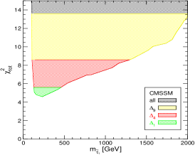
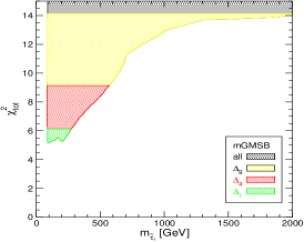
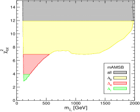
Figure 2: The mass of the lighter scalar tau is shown in the CMSSM (left), mGMSB (middle), mAMSB (right) scenario for $\mu>0$ with their respective total $\chi^{2}$. The region with $\Delta\chi^{2}:=\chi^{2}-\chi^{2}_{\rm min}<1$ is medium shaded (green), the $\Delta\chi^{2}<4$ region is dark shaded (red), and the $\Delta\chi^{2}<9$ region is light shaded (yellow). The rest of the scanned parameter space is given in black shading asbs3 .

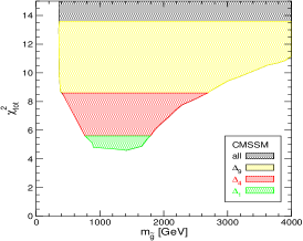
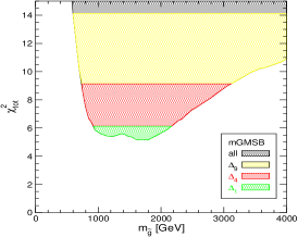
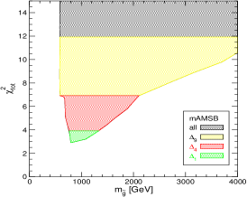
Figure 3: The mass of the gluino is shown in the CMSSM (left), mGMSB (middle), mAMSB (right) scenario for $\mu>0$ with their respective total $\chi^{2}$ asbs3 . The color coding is as in Fig. 2.

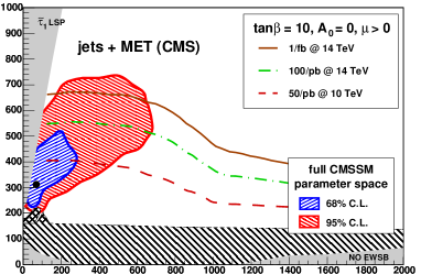
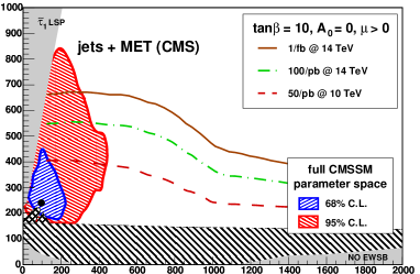
Figure 4: The $m_{0}$–$m_{1/2}$ plane in the CMSSM (left) and NUHM1 (right). The best-fit point is indicated by a filled circle, and the 68 (95)% C.L. contours from the fit as dark grey/blue (light grey/red) overlays, scanned over all $\tan\beta$ and $A_{0}$ values. The plot shows the $5\,\sigma$ discovery contours for jet + missing $E_{T}$ events at CMS with 1 fb^-1 at 14 TeV, 100 pb^-1 at 14 TeV and 50 pb^-1 at 10 TeV centre-of-mass energy (for $\tan\beta=10$ and $A_{0}=0$).

In Fig. 4 we show the prediction derived in Ref. mastercode2 for the CMSSM (left) and NUHM1 (right) parameters based on the fit of the EWPO, BPO and astrophysical data. The $m_{0}$–$m_{1/2}$ plane in the two scenarios is shown, where the best-fit point is indicated by a filled circle, and the 68 (95)% C.L. contours from the fit as dark grey/blue (light grey/red) overlays, scanned over all $\tan\beta$ and $A_{0}$ values. The CMSSM best-fit point has the parameters $m_{0}=60$ GeV, $m_{1/2}=310$ GeV, $A_{0}=240$ GeV and $\tan\beta=11$, the NUHM1 best-fit point has $m_{0}=100$ GeV, $m_{1/2}=240$ GeV, $A_{0}=-930$ GeV, $\tan\beta=7$, $m_{H}^{2}=-6.9\times 10^{5}$ GeV². Furthermore shown are the $5\,\sigma$ discovery contours for jet + missing $E_{T}$ events at CMS with 1 fb^-1 at 14 TeV, 100 pb^-1 at 14 TeV and 50 pb^-1 at 10 TeV centre-of-mass energy. They have been obtained for $\tan\beta=10$ and $A_{0}=0$, but do not vary significantly with these two parameters. The dark shaded area in Fig. 4 at low $m_{0}$ and high $m_{1/2}$ is excluded due to a scalar tau LSP, the light shaded areas at low $m_{1/2}$ do not exhibit electroweak symmetry breaking. The nearly horizontal line at $m_{1/2}\approx 160$ GeV has $m_{\tilde{\chi}_{1}^{\pm}}=103$ GeV, and the area below is excluded by LEP searches. Just above this contour at low $m_{0}$ in the lower panel is the region that is excluded by trilepton searches at the Tevatron. One can see that the for the CMSSM as well as for the NUHM1 the 68% likelihood contour is well covered by the 14 TeV/100 pb^-1 discovery reach, and even the 10 TeV/50 pb^-1 reach would be sufficient to discover SUSY at the best-fit point. This offers very good prospects for the initial LHC running.

3 CONSTRAINING $M_{h}$

Since the lightest MSSM Higgs boson mass can be predicted in terms of the other model parameters (see Refs. PomssmRep ; HiggsReviews for reviews), its preferred value can be fitted to the EWPO (and BPO) data, similar to the “Blue Band” plot in the SM LEPEWWG . For these analyses it is crucial not to include the $\chi^{2}$ contribution of $M_{h}$ itself into the fit.

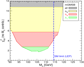
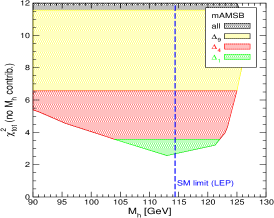
Figure 5: The $M_{h}$ values in the CMSSM (left), mGMSB (middle) and mAMSB (right) scenarios for $\mu>0$ with their respective $\chi^{2}$, where the $\chi^{2}$ contribution of the $M_{h}$ itself has been left out. The color coding is as in Fig. 2. The SM limit of $114.4\,\,\mathrm{GeV}$ obtained at LEP is indicated with a dashed (blue) line.

Figure 6: Left: Scan of the lightest Higgs boson mass versus $\Delta\chi^{2}$. The curve is the result of a CMSSM fit using all of the available constraints (see text). The direct limit on $M_{h}$ from LEP LEPHiggsSM ; LEPHiggsMSSM is not included. The red (dark gray) band represents the total theoretical uncertainty from unknown higher-order corrections, and the dark shaded area on the right above $127\,\,\mathrm{GeV}$ is theoretically inaccessible (see text). Right: Scan of the Higgs boson mass versus $\Delta\chi^{2}$ for the SM (blue/light gray), as determined by LEPEWWG using all available electroweak constraints, and for comparison, with the CMSSM scan superimposed (red/dark gray).

We first review the results obtained in Ref. asbs3 , where the three soft-SUSY breaking scenarios CMSSM, mGMSB and mAMSB are compared. As described above, the CDM has not been considered here. In Fig. 5. $M_{h}$ is shown in the CMSSM (left), mGMSB (middle) and mAMSB (right) scenarios for $\mu>0$ with the corresponding $\chi^{2}$, where the $\chi^{2}$ contribution of $M_{h}$ itself has been left out. In this way the plot shows the indirect predictions for $M_{h}$ without imposing the bounds from the Higgs boson searches at LEP LEPHiggsSM ; LEPHiggsMSSM . In all three scenarios a shallow minimum can be observed. The $\Delta\chi^{2}<1$ regions are in the intervals of $M_{h}=98\ldots 111\,\,\mathrm{GeV}$ (CMSSM), $97\ldots 112\,\,\mathrm{GeV}$ (mGMSB) and $104\ldots 122\,\,\mathrm{GeV}$ (mAMSB). In all three scenarios the $\Delta_{4}$ regions extend beyond the LEP limit of $M_{h}>114.4\,\,\mathrm{GeV}$ at the 95% C.L. shown as dashed (blue) line in Fig. 5 (which is valid for the three soft SUSY-breaking scenarios, see Refs. asbs1 ; ehow1 ). All three scenarios have a significant part of the parameter space with a relatively low total $\chi^{2}$ that is in agreement with the bounds from Higgs-boson searches at LEP. Especially within the mAMSB scenario the $\Delta\chi^{2}<1$ region extends beyond the LEP bound of $114.4\,\,\mathrm{GeV}$.

The fact that the minimum in Fig. 5 is relatively sharply defined is a general consequence of the MSSM, where the neutral Higgs boson mass is not a free parameter. The theoretical upper bound $M_{h}\;\raisebox{-3.00003pt}{$\stackrel{{\scriptstyle\displaystyle<}}{{\sim}}$}\;125\,\,\mathrm{GeV}$ (depending somewhat on the GUT scenario) explains the sharper rise of the $\Delta\chi^{2}$ at large $M_{h}$ values. In the SM, $M_{H}^{\mathrm{SM}}$ is a free parameter and only enters (at leading order) logarithmically in the prediction of the precision observables. In the MSSM this logarithmic dependence is still present, but in addition $M_{h}$ depends on $m_{t}$ and the SUSY parameters, mainly from the scalar top sector. The low-energy SUSY parameters in turn are all connected via RGEs to the GUT scale parameters. The sensitivity on $M_{h}$ in the analysis of Ref. asbs3 (and also in Ref. mastercode1 , see below) is therefore the combination of the indirect constraints on the few free GUT parameters and $\tan\beta$ and the fact that $M_{h}$ is directly predicted in terms of these parameters.

A fit as close as possible to the SM fit for $M_{H}^{\mathrm{SM}}$ has been performed in Ref. mastercode1 . All EWPO as in the SM LEPEWWG (except $\Gamma_{W}$, which has a minor impact) were included, supplemented by the CDM constraint, the $(g-2)_{\mu}$ results and the ${\rm BR}(b\to s\gamma)$ constraint. The top quark mass used in this fit was $m_{t}=170.9\pm 1.8\,\,\mathrm{GeV}$. The $\chi^{2}$ is minimized with respect to all CMSSM parameters for each point of this scan. Therefore, $\Delta\chi^{2}=1$ represents the 68% confidence level uncertainty on $M_{h}$. Since the direct Higgs boson search limit from LEP is not used in this scan the lower bound on $M_{h}$ arises as a consequence of indirect constraints only, as in the SM fit.

In the left plot of Fig. 6 mastercode1 the $\Delta\chi^{2}$ is shown as a function of $M_{h}$ in the CMSSM. The area with $M_{h}\geq 127$ is theoretically inaccessible. The right plot of Fig. 6 shows the red band parabola from the CMSSM in comparison with the blue band parabola from the SM. There is a well defined minimum in the red band parabola, leading to a prediction of mastercode1 $M_{h}^{\rm CMSSM}=110^{+8}_{-10}\;{\small{\rm(exp)}}\pm 3\;{\small{\rm(theo)}\,\,\mathrm{GeV},}$ where the first, asymmetric uncertainties are experimental and the second uncertainty is theoretical (from the unknown higher-order corrections to $M_{h}$ mhiggsAEC ; PomssmRep ). The most striking feature is that even without the direct experimental lower limit from LEP of $114.4\,\,\mathrm{GeV}$ the CMSSM prefers a Higgs boson mass which is quite close to and compatible with this bound.

References

- (1) H. Nilles, Phys. Rept. 110 (1984) 1; H. Haber and G. Kane, Phys. Rept. 117 (1985) 75; R. Barbieri, Riv. Nuovo Cim. 11 (1988) 1.
- (2) W. Yao et al. [Particle Data Group Collaboration], J. Phys. G 33 (2006) 1.
- (3) S. Heinemeyer, W. Hollik and G. Weiglein, Phys. Rept. 425 (2006) 265 [arXiv:hep-ph/0412214].
- (4) S. Heinemeyer, W. Hollik, D. Stöckinger, A.M. Weber and G. Weiglein, JHEP 0608 (2006) 052 [arXiv:hep-ph/0604147].
- (5) S. Heinemeyer, W. Hollik, A.M. Weber and G. Weiglein, JHEP 0804 (2008) 039 [arXiv:0710.2972 [hep-ph]].
- (6) LEP Higgs working group, Phys. Lett. B 565 (2003) 61 [arXiv:hep-ex/0306033].
- (7) [Tevatron Electroweak Working Group and CDF Collaboration and D0 Collab], arXiv:0808.1089 [hep-ex].
- (8) S. Heinemeyer, W. Hollik and G. Weiglein, Eur. Phys. J. C 9 (1999) 343 [arXiv:hep-ph/9812472].
- (9) G. Degrassi, S. Heinemeyer, W. Hollik, P. Slavich and G. Weiglein, Eur. Phys. J. C 28 (2003) 133 [arXiv:hep-ph/0212020].
-
(10)
LEP Electroweak Working Group, see:
lepewwg.web.
cern.ch/LEPEWWG/Welcome.html . - (11) Tevatron Electroweak Working Group, see: tevewwg.fnal.gov .
- (12) G. Isidori, F. Mescia, P. Paradisi and D. Temes, Phys. Rev. D 75 (2007) 115019 [arXiv:hep-ph/0703035].
- (13) E. Barberio et al. [Heavy Flavour Averaging Group (HFAG)], hep-ex/0603003, see slac.stanford.edu/xorg/hfag/ .
- (14) J. Dunkley et al. [WMAP Collaboration], arXiv:0803.0586 [astro-ph].
- (15) J. Ellis, S. Heinemeyer, K. Olive and G. Weiglein, JHEP 0502 (2005) 013 [arXiv:hep-ph/0411216].
- (16) J. Ellis, S. Heinemeyer, K. Olive and G. Weiglein, JHEP 0605 (2006) 005 [arXiv:hep-ph/0602220].
- (17) J. Ellis, S. Heinemeyer, K. Olive, A.M. Weber and G. Weiglein, JHEP 0708 (2007) 083 [arXiv:0706.0652 [hep-ph]].
- (18) J. Ellis, K. Olive, Y. Santoso and V. Spanos, Phys. Rev. D 69 (2004) 095004 [arXiv:hep-ph/0310356]; B. Allanach and C. Lester, Phys. Rev. D 73 (2006) 015013 [arXiv:hep-ph/0507283]; B. Allanach, Phys. Lett. B 635 (2006) 123 [arXiv:hep-ph/0601089]; R. de Austri, R. Trotta and L. Roszkowski, JHEP 0605 (2006) 002 [arXiv:hep-ph/0602028]; JHEP 0704 (2007) 084 [arXiv:hep-ph/0611173]; JHEP 0707 (2007) 075 [arXiv:0705.2012 [hep-ph]]; B. Allanach, C. Lester and A. M. Weber, JHEP 0612 (2006) 065 [arXiv:hep-ph/0609295]; JHEP 0708 (2007) 023 [arXiv:0705.0487 [hep-ph]]; F. Feroz, B. Allanach, M. Hobson, S. AbdusSalam, R. Trotta and A. M. Weber, arXiv:0807.4512 [hep-ph]; S. Heinemeyer, arXiv:hep-ph/0611372.
- (19) B. Allanach and D. Hooper, arXiv:0806.1923 [hep-ph].
- (20) O. Buchmueller et al., Phys. Lett. B 657 (2007) 87 [arXiv:0707.3447 [hep-ph]].
- (21) O. Buchmueller et al., arXiv:0808.4128 [hep-ph].
-
(22)
R. Trotta,
talk given at Tools08, Munich, July 2008, see:
indico.cern.ch/getFile.py/access?
contribId=43&sessionId=20&resId=0&
materialId=slides&confId=35476, based on work in collab. with L. Roszkowski and R. de Austri. - (23) J. Ellis, S. Heinemeyer, K. Olive and G. Weiglein, Phys. Lett. B 653 (2007) 292 [arXiv:0706.0977 [hep-ph]]; J. Ellis, T. Hahn, S. Heinemeyer, K. Olive and G. Weiglein, JHEP 0710 (2007) 092 [arXiv:0709.0098 [hep-ph]].
- (24) S. Heinemeyer, X. Miao, S. Su and G. Weiglein, JHEP 0808 (2008) 087 [arXiv:0805.2359 [hep-ph]].
- (25) S. Heinemeyer, M. Mondragón and G. Zoupanos, arXiv:0712.3630 [hep-ph]; arXiv:0809.2397 [hep-ph].
- (26) K. Cranmer, Y. Fang, B. Mellado, S. Paganis, W. Quayle and S. Wu, hep-ph/0401148; K. Assamagan, Y. Coadou and A. Deandrea, Eur. Phys. J. direct C 4 (2002) 9 [arXiv:hep-ph/0203121]; K. Assamagan and N. Gollub, Eur. Phys. J. C 39S2 (2005) 25 [arXiv:hep-ph/0406013]; M. Baarmand, M. Hashemi and A. Nikitenko, CMS Note 2006/056; R. Kinnunen, CMS Note 2006/100; S. Gennai, S. Heinemeyer, A. Kalinowski, R. Kinnunen, S. Lehti, A. Nikitenko and G. Weiglein, Eur. Phys. J. C 52 (2007) 383 [arXiv:0704.0619 [hep-ph]]. M. Hashemi, S. Heinemeyer, R. Kinnunen, A. Nikitenko and G. Weiglein, arXiv:0804.1228 [hep-ph]; S. Heinemeyer, A. Nikitenko, G. Weiglein, arXiv:0809.2396 [hep-ph].
- (27) B. Allanach and C. Lester, Comput. Phys. Commun. 179 (2008) 256 [arXiv:0705.0486 [hep-ph]].
- (28) S. Heinemeyer, Int. J. Mod. Phys. A 21 (2006) 2659 [arXiv:hep-ph/0407244]; A. Djouadi, Phys. Rept. 459 (2008) 1 [arXiv:hep-ph/0503173].
- (29) LEP Higgs working group, Eur. Phys. J. C 47 (2006) 547 [arXiv:hep-ex/0602042].
- (30) S. Ambrosanio, A. Dedes, S. Heinemeyer, S. Su and G. Weiglein, Nucl. Phys. B 624 (2001) 3 [arXiv:hep-ph/0106255].
- (31) J. Ellis, S. Heinemeyer, K. Olive and G. Weiglein, Phys. Lett. B 515 (2001) 348 [arXiv:hep-ph/0105061].