A cosmic abundance standard: chemical homogeneity of the solar neighbourhood
and the ISM dust-phase composition

Abstract

A representative sample of unevolved early B-type stars in nearby OB associations and the field is analysed to unprecedented precision using NLTE techniques. The resulting chemical composition is found to be more metal-rich and much more homogeneous than indicated by previous work. A rms scatter of $\sim$10% in abundances is found for the six stars (and confirmed by six evolved stars), the same as reported for ISM gas-phase abundances. A cosmic abundance standard for the present-day solar neighbourhood is proposed, implying mass fractions for hydrogen, helium and metals of $X$ $=$ 0.715, $Y$ $=$ 0.271 and $Z$ $=$ 0.014. Good agreement with solar photospheric abundances as reported from recent 3D radiative-hydrodynamical simulations of the solar atmosphere is obtained. As a first application we use the cosmic abundance standard as a proxy for the determination of the local ISM dust-phase composition, putting tight observational constraints on dust models.

1. Introduction

The Sun is unique among the stars because independent indicators allow its chemical composition to be constrained with a precision unmatched for any other star. This can be done by spectroscopic analysis of its photosphere and by measurement of solar wind and solar energetic particles. Solar nebula abundances can be determined from CI chondrites, which are unaltered since the formation of the system. The wealth of information established the Sun as the principal standard for the chemical composition of cosmic matter (e.g. Grevesse & Sauval 1998, GS98; Holweger 2001; Asplund et al 2005, AGS05). However, is a 4.6 Gyr old star indeed representative of the cosmic matter in its neighbourhood at present?

Ideal indicators for pristine abundances are unevolved early B-stars of spectral types B0–B2. Slowly rotating stars are preferred as their photospheres should be essentially unaffected by mixing of CN-processed material (Maeder & Meynet, 2000). The atmospheres of early B-stars are also unaffected by atomic diffusion that gives rise to peculiarities of metal abundances in many later-type stars (e.g. Smith, 1996). A major practical advantage is also their relatively simple photospheric physics, which is represented well by classical model atmospheres, unaffected by complications such as stellar winds or convection.

As a consequence, early B-stars in the solar neighbourhood were subject of several NLTE studies in the past (e.g. Gies & Lambert, 1992; Kilian, 1992, 1994; Cunha & Lambert, 1994; Daflon et al., 1999, 2001a, 2001b, 2003; Lyubimkov et al., 2004, 2005). Overall, they found a wide range of abundances, by about a factor $\sim$10, and an average metallicity of only $\sim$2/3 solar (GS98). Hence, the impression arose that the solar neighbourhood is chemically highly heterogeneous, and the Sun anomalously metal-rich compared to young stars.

Both findings are problematic in terms of Galactic chemical evolution. Dispersal of stellar nucleosynthesis products increases the metallicity over time (e.g. Chiappini et al., 2003) and hydrodynamic mixing tends to homogenize the interstellar medium (ISM) locally (Edmunds, 1975). Characteristic timescales for homogenization are short, ranging from 10⁶–10⁸ yrs on scales of 100-1000 pc (Roy & Kunth, 1995).

In contrast to the young stars the interstellar gas shows a high degree of chemical homogeneity in the solar neighbourhood (Sofia, 2004), with the rms scatter of mean abundances being $\sim$10%. However, the ISM gas phase is not suitable as a tracer for cosmic abundances because of selective depletion of elements onto dust grains. Here we reinvestigate the conundrum of inhomogeneous stellar vs. homogeneous ISM gas-phase abundances in the solar neighbourhood, motivated by the finding of homogeneous B-star abundances for carbon (see detailed analysis by Nieva & Przybilla, 2008, NP08).

2. Sample Analysis

Six bright and apparently slow-rotating early B stars in the solar neighbourhood – randomly distributed in OB associations and in the field, and covering a wide range of stellar parameters – were observed in early 2005 at ESO/La Silla, using FEROS on the 2.2 m telescope. Spectra with broad wavelength coverage and resolving power $\lambda/\Delta\lambda$ $\approx$ 48 000 were obtained, at very high-S/N (up to $\sim$800 in the $B$-band).

Table 1Stellar parameters & elemental abundances

	HR 6165 (catalog HR 6165)	HR 3055 (catalog HR 3055)	HR 1861 (catalog HR 1861)	HR 2928 (catalog HR 2928)	HR 3468 (catalog HR 3468)	HR 5285 (catalog HR 5285)
Sp. Type	B0.2 V	B0 III	B1 IV	B1 IV	B1.5 III	B2 V
Association	Sco Cen	Field	Ori OB1b	Field	Field	Sco Cen
$d$ (pc)	152$\pm$20	438$\pm$57	450$\pm$59	481$\pm$63	319$\pm$41	155$\pm$20
$T_{\rm eff}$ (K)	32000$\pm$300	31200$\pm$300	27000$\pm$300	26300$\pm$300	22900$\pm$300	20800$\pm$300
$\log g$ (cgs)	4.30$\pm$0.05	3.95$\pm$0.05	4.12$\pm$0.05	4.15$\pm$0.05	3.60$\pm$0.05	4.22$\pm$0.05
$\xi$ (km s-1)	5$\pm$1	8$\pm$1	3$\pm$1	3$\pm$1	5$\pm$1	3$\pm$1
$v\sin i$ (km s-1)	4$\pm$4	29$\pm$4	12$\pm$1	14$\pm$1	11$\pm$2	18$\pm$1
$\zeta$ (km s-1)	4$\pm$4	37$\pm$8	$\cdots$	20$\pm$2	20$\pm$1	$\cdots$
$\varepsilon$(He)a	10.99$\pm$0.05 (20)	10.94$\pm$0.05 (16)	10.99$\pm$0.05 (14)	10.99$\pm$0.05 (14)	10.99$\pm$0.05 (14)	10.99$\pm$0.05 (13)
$\varepsilon$(C ii)b	8.27$\pm$0.14 (13)	8.35$\pm$0.08 (10)	8.32$\pm$0.10 (19)	8.28$\pm$0.08 (18)	8.36$\pm$0.10 (17)	8.32$\pm$0.08 (20)
$\varepsilon$(C iii)b	8.31$\pm$0.11 (17)	8.30$\pm$0.05   (7)	8.36$\pm$0.03 (11)	8.27$\pm$0.02   (5)	8.47$\pm$0.04   (2)	8.42$\pm$0.06   (2)
$\varepsilon$(C iv)b	8.34   (2)	8.45   (2)	$\cdots$	$\cdots$	$\cdots$	$\cdots$
$\varepsilon$(N ii)c	8.16$\pm$0.12 (73)	7.77$\pm$0.08 (23)	7.75$\pm$0.09 (61)	8.00$\pm$0.12 (61)	7.92$\pm$0.10 (56)	7.76$\pm$0.08 (47)
$\varepsilon$(O i)d	$\cdots$	$\cdots$	8.82$\pm$0.03   (3)	8.83$\pm$0.05   (5)	8.82$\pm$0.03   (7)	8.79$\pm$0.05   (7)
$\varepsilon$(O ii)e	8.77$\pm$0.08 (51)	8.79$\pm$0.10 (41)	8.74$\pm$0.11 (52)	8.74$\pm$0.09 (46)	8.80$\pm$0.09 (40)	8.71$\pm$0.05 (45)
$\varepsilon$(Ne i)f	8.12$\pm$0.05   (2)	$\cdots$	8.12$\pm$0.08   (9)	8.11$\pm$0.09   (9)	8.05$\pm$0.09 (10)	8.07$\pm$0.07 (14)
$\varepsilon$(Ne ii)f	8.14$\pm$0.07 (16)	8.07$\pm$0.07   (8)	8.08$\pm$0.09 (14)	8.03$\pm$0.12   (8)	8.06$\pm$0.03   (2)	$\cdots$
$\varepsilon$(Mg ii)g	7.62$\pm$0.03   (3)	7.60$\pm$0.01   (2)	7.58$\pm$0.10   (6)	7.56$\pm$0.03   (3)	7.51$\pm$0.10   (6)	7.50$\pm$0.05   (4)
$\varepsilon$(Si ii)h	$\cdots$	$\cdots$	7.47$\pm$0.17   (2)	7.56$\pm$0.08   (2)	7.51$\pm$0.10   (5)	7.22$\pm$0.13   (6)
$\varepsilon$(Si iii)h	7.50$\pm$0.08   (8)	7.48$\pm$0.08   (6)	7.46$\pm$0.11   (9)	7.52$\pm$0.11   (8)	7.53$\pm$0.17   (7)	7.29$\pm$0.05   (9)
$\varepsilon$(Si iv)h	7.50$\pm$0.04 (10)	7.51$\pm$0.18   (5)	7.50$\pm$0.08   (3)	7.48$\pm$0.14   (2)	7.50$\pm$0.04   (2)	$\cdots$
$\varepsilon$(Fe ii)i	$\cdots$	$\cdots$	$\cdots$	$\cdots$	7.38   (1)	7.38   (1)
$\varepsilon$(Fe iii)j	7.38$\pm$0.12 (17)	7.49$\pm$0.12   (5)	7.44$\pm$0.09 (33)	7.48$\pm$0.10 (30)	7.42$\pm$0.12 (36)	7.40$\pm$0.09 (32)

$\varepsilon({\rm El})$ $=$ $\log({\rm El}/{\rm H})$ $+$ 12, with rms uncertainties and number of analysed lines in parentheses. NLTE model atoms: H: Przybilla & Butler (2004); ^a Przybilla (2005); ^b Nieva & Przybilla (2006, 2008); ^c Przybilla & Butler (2001); ^d Przybilla et al. (2000); ^e Becker & Butler (1988),updated; ^f Morel & Butler (2008), $gf$-values of Froese Fischer & Tachiev (2004) for Ne I; ^g Przybilla et al. (2001); ^h Becker & Butler (1990), extended & updated; ⁱ Becker (1998); ^j Morel et al. (2007)

The quantitative analysis of the sample stars was carried out following the hybrid NLTE approach discussed by Nieva & Przybilla (2007, NP07) and NP08. In brief, line-blanketed LTE model atmospheres were computed with ATLAS9 (Kurucz, 1993) and NLTE line-formation calculations were performed using updated versions of our codes Detail and Surface. State-of-the-art model atoms were adopted (see Table 1), which allow atmospheric parameters and elemental abundances to be obtained with high accuracy.

Figure 1.— Comparison with stellar evolution tracks (Meynet & Maeder, 2003). Observed and predicted N/C ratios (by mass) are indicated. The inset shows the location of the sample stars as projected on the Galactic plane, with the solar neighbourhood (as considered here) schematically outlined. Crosses denote positions of BA-SGs from the control sample (see text).

Multiple independent spectroscopic indicators were considered simultaneously for the determination of the atmospheric parameters, effective temperature $T_{\rm eff}$ and surface gravity $\log g$: all Stark-broadened Balmer lines and 4–6 ionization equilibria, of He I/II, C II/III/IV, O I/II, Ne I/II, Si II/III/IV and Fe II/III. Also, the observed spectral energy distributions were reproduced (Nieva & Przybilla, 2006). The redundancy helps to avoid systematic errors. The microturbulent velocity $\xi$ was determined by demanding that abundances be independent of line equivalent widths. Elemental abundances $\varepsilon$(El), rotational velocity $v\sin i$ and macroturbulence $\zeta$ were determined from fits to individual line profiles. The results are summarized in Table 1. Stellar parameters and He and C abundances are identical with those derived by NP07/NP08, except for HR 5285, where consideration of additional ionization equilibria indicated small revisions, though agreement is obtained within the mutual uncertainties. Spectral types and spectroscopic distances are also given in Table 1, agreeing well with HIPPARCOS parallaxes (HR 6165, HR 5285) or with the association distance (HR 1861). The positions of the stars in the $T_{\rm eff}$–$\log g$-plane are indicated in Fig. 1, where a comparison with evolution tracks is made. An overview of the location of the stars in the solar vicinity is also given there.

The uncertainties in the atmospheric parameters were determined from the quality of the simultaneous fits to all diagnostic indicators. Statistical uncertainties for abundances were obtained from the individual line data (rms values). Systematic errors in the abundances due to uncertainties in atmospheric parameters, atomic data and the quality of the spectrum are $\sim$0.1 dex (NP08, Przybilla et al., 2006), i.e. about as large as the statistical errors.

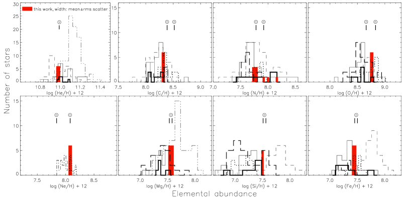
Figure 2.— Comparison of chemical abundance studies (NLTE) of B-stars in the solar neighbourhood. Red bars: present work; full line and thick full line (for the same stars as in our work): Kilian (1992, 1994); dotted: Cunha & Lambert (1994), Cunha et al. (2006) for Ne; short-dashed: Gies & Lambert (1992), excluding bright giants and SGs; long-dashed: Daflon et al. (1999, 2001a, 2001b, 2003); dot-dashed: Morel & Butler (2008); triple-dot-dashed: Lyubimkov et al. (2004, 2005). Bin width is $\sigma$/2 of the individual studies. Iron abundances in LTE in all previous work. HR 5285 is Si-peculiar and therefore excluded from the silicon mean abundance. Solar abundances ($\odot$): GS98 & AGS05 (lower values). The panel for C is reproduced from NP08 for completeness. See the text for details.

Our analysis of each individual star differs from standard studies in two main respects: i) practically all (unblended) lines of the ion spectra are analyzed instead of a few selected ‘good’ lines thus avoiding selection effects, and ii) all parameter indicators (in particular the ionization equilibria) are closely matched simultaneously, which has never been achieved before. As a result, practically the entire observed stellar spectrum is reproduced closely by the spectral synthesis, see NP07, NP08, Przybilla et al. (2008) for examples. This is facilitated by the use of critically evaluated data in the model atom construction and a (time-consuming) iterative approach for a precise determination of the stellar parameters (NP08). Less accurate photometric $T_{\rm eff}$-estimates as adopted in most previous work are avoided, as $T_{\rm eff}$-uncertainties are often the most important sources of systematic error in the abundance derivation, next to ill-chosen atomic data (NP08) and $\log g$-uncertainties (NP07).

3. Chemical homogeneity of the solar vicinity

The status of previous NLTE abundance studies of early B-stars in the solar neighbourhood (covering clusters, associations and field stars) is illustrated in Fig. 2. A wide range of abundance values is found for most elements, typically spanning $\sim$1 dex (for comparison, such a range is bridged by the cumulative effect of $\sim$13 Gyrs of Galactochemical evolution, see e.g. Fig. 2 of Chiappini et al., 2003). Moreover, the abundance distributions peak in most cases at sub-solar values, in particular when referring to the solar composition of GS98. Exceptions are He, where most previous studies find values on average larger than solar, and Ne (about solar, GS98, from two very recent studies; see also Lanz et al. 2008 for the case of Ar). Several of these older B-star studies were combined by Snow & Witt (1996) and Sofia & Meyer (2001, SM01, see Table 2) to derive a reference composition, inevitably resulting in sub-solar average values and a large rms scatter. The former discrepancy has since been largely removed from a re-evaluation of solar abundances (AGS05). However, the status quo in terms of Galactochemical evolution can only be understood by invoking and fine-tuning extra processes such as infall/outflow of material and local retention of supernova products by large amounts.

On the other hand, our sample of early B-stars implies a high degree of homogeneity for elemental abundances in the solar neighbourhood, with a scatter of $\sim$10%, and absolute values of about solar (GS98 and/or AGS05, see Fig. 2 and Table 2). The only exception is N, which is most sensitive to mixing of the atmospheric layers with CN-processed material (e.g. Maeder & Meynet, 2000). In this case the pristine N abundance may be indicated by the 3 objects with the lowest value, implying a pristine N/C ratio of 0.31$\pm$0.05 (by mass; error bar accounts for additional uncertainties).

Although our sample is small, we regard it as representative for the early B-star population in the solar neighbourhood. The stars sample the relevant portion of the H-burning phase of the objects in the HRD in terms of $T_{\rm eff}$ and $\log g$ (see Fig. 1). They also sample one hemisphere of the solar neighbourhood (inset of Fig. 1), half of them located in OB associations and the other half in the field. All six stars were analyzed by Kilian (1992, 1994) before, typically spanning the entire abundance range in her sample of 21 stars (see Fig. 2). We therefore also find a chance selection of stars with similar chemical composition for our sample unlikely. The wide abundance ranges found in previous work reflect the lower accuracy of the analyses, while shifts of the abundance distributions relative to each other reflect systematics, with different temperature scales being the most important among these. Our results are supported further by a control sample of six BA-type supergiants (BA-SGs, Fig. 1), for which mean values of $\varepsilon$(O) = 8.80$\pm$0.02 and $\varepsilon$(Mg) = 7.55$\pm$0.07 were derived using the same analysis methodology as applied here (Przybilla et al., 2006; Firnstein, 2006).

The finding of chemical homogeneity for our sample is in excellent accordance with results from the analysis of the ISM gas-phase in the solar neighbourhood (Sofia, 2004, and references therein) and with theory regarding the efficiency of hydrodynamic mixing in the ISM (Edmunds, 1975; Roy & Kunth, 1995). Excellent agreement is also obtained with elemental abundances in the Orion nebula (Esteban et al., 2004, E04, see Table 2), with the exception of C, which may be a consequence of the atomic data used in the Orion analysis (see NP08 for the stellar case) plus overestimated dust corrections.

In the following we briefly investigate the impact of this cosmic abundance standard on important topics of contemporary astrophysics.

Table 2Chemical composition of different object classes in the solar neighbourhood and of the Sun

	cosmic standard		Orion		Young	ISM	ISM
Elem.	B stars – this work		gas+dustb	B starsc	F&G starsc	gas	dustd	Sune/f
He	10.98$\pm$0.02/	$\cdots$ a	10.988$\pm$0.003	$\cdots$	$\cdots$	$\cdots$	$\cdots$	10.99$\pm$0.02
C	8.32$\pm$0.03/	209$\pm$15	8.52$\pm$0.02	8.28$\pm$0.17	8.55$\pm$0.10	8.15$\pm$0.06g	68$\pm$26	8.52$\pm$0.06/	8.39$\pm$0.05
N	7.76$\pm$0.05/	58$\pm$47	7.73$\pm$0.09	7.81$\pm$0.21	$\cdots$	7.79$\pm$0.03h	$\cdots$	7.92$\pm$0.06/	7.78$\pm$0.06
O	8.76$\pm$0.03/	575$\pm$41	8.73$\pm$0.03	8.54$\pm$0.16	8.65$\pm$0.15	8.59$\pm$0.01i	186$\pm$42	8.83$\pm$0.06/	8.66$\pm$0.05
Ne	8.08$\pm$0.03/	120$\pm$49	8.05$\pm$0.07	$\cdots$	$\cdots$	$\cdots$	$\cdots$	8.08$\pm$0.06/	7.84$\pm$0.06
Mg	7.56$\pm$0.05/	36$\pm$44	$\cdots$	7.36$\pm$0.13	7.63$\pm$0.17	6.17$\pm$0.02j	34.8$\pm$4.4	7.58$\pm$0.05/	7.53$\pm$0.09
Si	7.50$\pm$0.02/	32$\pm$41	$\cdots$	7.27$\pm$0.20	7.60$\pm$0.14	6.35$\pm$0.05j	29.6$\pm$2.2	7.55$\pm$0.05/	7.51$\pm$0.04
Fe	7.44$\pm$0.04/	28$\pm$43	$\cdots$	7.45$\pm$0.26	7.45$\pm$0.12	5.41$\pm$0.04j	27.3$\pm$2.7	7.50$\pm$0.05/	7.45$\pm$0.05

^a in units of $\log({\rm El}/{\rm H})+12$ / atoms per 10⁶ H nuclei – computed from average star abundances (mean values over all individual lines per element, equal weight per line); ^b E04; ^c SM01; ^d difference between the cosmic standard and ISM gas-phase abundances, in units of atoms per 10⁶ H nuclei; ^e/f GS98/AGS05, photospheric values; ^g Sofia (2004); ^h Meyer et al. (1997), corrected accordingly to Jensen et al. (2007); ⁱ Cartledge et al. (2004); ^j Cartledge et al. (2006)

4. The cosmic abundance standard: first applications

In general, excellent agreement of our B-star abundances with solar values from recent 3D radiative-hydrodynamical simulations of the solar atmosphere (AGS05) is obtained. The oxygen value falls between GS98 and AGS05 values and neon is compatible with GS98. This opens up new perspectives in the ongoing discussion on helioseismic constraints, chemical abundances and the solar interior model as reviewed by Basu & Antia (2008).

Our cosmic abundance standard also facilitates a precise determination of dust depletion in the local ISM for the primary constituents. The amount of material incorporated into dust grains is determined by the difference between our B-star abundances and the ISM gas-phase abundances, see Table 2. Accordingly, a composition poor in carbon but rich in oxygen and refractory elements is indicated.

Such studies were undertaken previously, using e.g. abundances of the Sun, of B stars and of young F & G stars (e.g. Snow & Witt, 1996, SM01, see Table 2) as proxies for the determination of the dust-phase composition, however with mixed success. In particular, B stars were rejected as reliable indicators as the derived abundances of material in dust at that time were too low to produce the observed interstellar extinction. Our study revives B stars as proxies of the ISM dust-phase composition, and even more so because of the extremely low abundance scatter compared to all other standards considered so far, except for the Sun.

The present results imply tight observational constraints on dust models in terms of carbon abundance. The observed properties of dust grains, as inferred from the interstellar extinction law, have to be produced by a rather small amount of carbon, posing a challenge to most dust models (see e.g. Snow & Witt, 1995). We can carry out an important consistency check, following Cartledge et al. (2006): the O predicted to be incorporated in grains from the observed Mg, Si and Fe dust abundances and a rudimentary dust model agrees with the derived O dust abundance within the mutual (small) uncertainties. For the rudimentary dust model we assume silicates to be predominantly MgSiO₃, with only a small fraction of Fe bound in silicates and only a small fraction being of olivine-like composition. The remaining Mg and Fe fraction is considered to be in oxide form (MgO, FeO, Fe₂O₃, Fe₃O₄), see e.g. Draine (2003) for a discussion of observational evidence.

Finally, we combine our B-star abundances with data for S, Cl and Ar from the analysis of the Orion nebula (E04) and solar meteoritic values for other abundant refractory elements (with $\varepsilon$(El) $\gtrsim$ 5, AGS05) to derive mass fractions for hydrogen, helium and the metals. Values of $X$ $=$ 0.715, $Y$ $=$ 0.271, $Z$ $=$ 0.014 and $Z/X$ $=$ 0.020 characterize the present-day cosmic matter in the solar neighbourhood (to be compared to protosolar values $X_{0}$ = 0.7133, $Y_{0}$ = 0.2735 and $Z_{0}$=0.0132, Grevesse et al., 2007). These combined abundances are our recommended values for a wide range of applications requiring an accurate knowledge of the chemical composition at present (e.g. for opacity calculations), examples being models of star/planet formation or stellar evolution (in particular of short-lived massive stars), or for the empirical calibration of Galactochemical evolution models.

References

- Asplund et al. (2005) Asplund, M., et al. 2005, ASP Conf. Ser., 336, 25 (AGS05)
- Basu & Antia (2008) Basu, S., & Antia, H. M. 2008, Phys. Rep., 457, 217
- Becker (1998) Becker, S. R. 1998, ASP Conf. Ser., 131, 137
- Becker & Butler (1988) Becker, S. R., & Butler, K. 1988, A&A, 201, 232
- Becker & Butler (1990) Becker, S. R., & Butler, K. 1990, A&A, 235, 326
- Cartledge et al. (2004) Cartledge, S. I. B., Lauroesch, J. T., et al. 2004, ApJ, 613, 1037
- Cartledge et al. (2006) Cartledge, S. I. B., Lauroesch, J. T., et al. 2006, ApJ, 641, 327
- Chiappini et al. (2003) Chiappini, C., Romano, D., & Matteucci, F. 2003, MNRAS, 339, 63
- Cunha & Lambert (1994) Cunha, K., & Lambert, D. L. 1994, ApJ, 426, 170
- Cunha et al. (2006) Cunha, K., Hubeny, I., & Lanz, T. 2006, ApJ, 647, L143
- Daflon et al. (1999) Daflon, S., Cunha, K., & Becker, S. R. 1999, ApJ, 522, 950
- Daflon et al. (2001a) Daflon, S., Cunha, K., Becker, S. R., & Smith, V. V. 2001a, ApJ, 552, 309
- Daflon et al. (2001b) Daflon, S., Cunha, K., Butler, K., & Smith, V. V. 2001b, ApJ, 563, 325
- Daflon et al. (2003) Daflon, S., Cunha, K., Smith, V. V., & Butler, K. 2003, A&A, 399, 525
- Draine (2003) Draine, B. T. 2003, ARA&A, 41, 241
- Edmunds (1975) Edmunds, M. G. 1975, Ap&SS, 32, 483
- Esteban et al. (2004) Esteban, C., et al. 2004, MNRAS, 355, 229 (E04)
- Firnstein (2006) Firnstein, M. 2006, Diploma Thesis, Univ. Erlangen-Nuremberg
- Froese Fischer & Tachiev (2004) Froese Fischer, C., & Tachiev, G. 2004, At. Data Nucl. Data Tables, 87, 1
- Gies & Lambert (1992) Gies, D. R., & Lambert, D. L. 1992, ApJ, 387, 673
- Grevesse & Sauval (1998) Grevesse, N., & Sauval, A. J. 1998, Space Sci. Rev., 85, 161 (GS98)
- Grevesse et al. (2007) Grevesse, N., Asplund, M., & Sauval, A. J. 2007, Space Sci. Rev., 130, 105
- Holweger (2001) Holweger, H. 2001, AIP Conf. Proc., 598, 23
- Jensen et al. (2007) Jensen, A. G., Rachford, B. L., & Snow, T. P. 2007, ApJ, 654, 955
- Kilian (1992) Kilian, J. 1992, A&A, 262, 17
- Kilian (1994) Kilian, J. 1994, A&A, 282, 867
- Kurucz (1993) Kurucz, R. L. 1993, CD-ROM 13 (Cambridge: SAO)
- Lanz et al. (2008) Lanz, T., Cunha, K., Holtzman, J., & Hubeny, I. 2008, ApJ, 678, 1342
- Lyubimkov et al. (2004) Lyubimkov, L. S., Rostopchin, S. I., Lambert, D. L. 2004, MNRAS, 351, 745
- Lyubimkov et al. (2005) Lyubimkov, L. S., Rostopchin, S. I., et al. 2005, MNRAS, 358, 193
- Maeder & Meynet (2000) Maeder, A., & Meynet, G. 2000, ARA&A, 38, 143
- Meyer et al. (1997) Meyer, D. M., Cardelli, J. A., & Sofia, U. J. 1997, ApJ, 490, L103
- Meynet & Maeder (2003) Meynet, G., & Maeder, A. 2003, A&A, 404, 975
- Morel & Butler (2008) Morel, T., & Butler, K. 2008, A&A, 487, 307
- Morel et al. (2007) Morel, T., Butler, K., Aerts, C., et al. 2007, A&A, 457, 651
- Nieva & Przybilla (2006) Nieva, M. F., & Przybilla, N. 2006, ApJ, 639, L39
- Nieva & Przybilla (2007) Nieva, M. F., & Przybilla, N. 2007, A&A, 467, 295 (NP07)
- Nieva & Przybilla (2008) Nieva, M. F., & Przybilla, N. 2008, A&A, 481, 199 (NP08)
- Przybilla (2005) Przybilla, N. 2005, A&A, 443, 293
- Przybilla & Butler (2001) Przybilla, N., & Butler, K. 2001, A&A, 379, 955
- Przybilla & Butler (2004) Przybilla, N., & Butler, K. 2004, ApJ, 609, 1181
- Przybilla et al. (2000) Przybilla, N., Butler, K., Becker, S. R., et al. 2000, A&A, 359, 1085
- Przybilla et al. (2001) Przybilla, N., Butler, K., Becker, S. R., Kudritzki, R. P. 2001, A&A, 369, 1009
- Przybilla et al. (2006) Przybilla, N., Butler, K., Becker, S. R., Kudritzki, R. P. 2006, A&A, 445, 1099
- Przybilla et al. (2008) Przybilla, N., Nieva, M. F., Heber, U., Butler, K. 2008, ApJ, 684, L103
- Roy & Kunth (1995) Roy, J.-R., & Kunth, D. 1995, A&A, 294, 432
- Smith (1996) Smith, K. C. 1996, Ap&SS, 237, 77
- Sofia (2004) Sofia, U. J. 2004, ASP Conf. Ser., 309, 393
- Sofia & Meyer (2001) Sofia, U. J., & Meyer, D. M. 2001, ApJ, 554, L221 (SM01)
- Snow & Witt (1995) Snow, T. P., & Witt, A. N. 1995, Science, 270, 1455
- Snow & Witt (1996) Snow, T. P., & Witt, A. N. 1996, ApJ, 468, L65