Stellar Velocity Distribution in Galactic Disks

Abstract

We present numerical studies of the properties of the stellar velocity distribution in galactic disks which have developed a saturated, two-armed spiral structure. In previous papers we used the Boltzmann moment equations (BME) up to second order for our studies of the velocity structure in self-gravitating stellar disks. A key assumption of our BME approach is the zero-heat flux approximation, i.e. the neglection of third order velocity terms. We tested this assumption by performing test particle simulations for stars in a disk galaxy subject to a rotating spiral perturbation. As a result we corroborated qualitatively the complex velocity structure found in the BME approach. It turned out that an equilibrium configuration in velocity space is only slowly established on a typical timescale of 5 Gyrs or more. Since many dynamical processes in galaxies (like the growth of spirals or bars) act on shorter timescales, pure equilibrium models might not be fully appropriate for a detailed comparison with observations like the local Galactic velocity distribution. Third order velocity moments were typically small and uncorrelated over almost all of the disk with the exception of the 1:4 resonance region (UHR). Near the UHR (normalized) fourth and fifth order velocity moments are still of the same order as the second and third order terms. Thus, at the UHR higher order terms are not negligible.

1 Introduction

It is long known that the velocity distribution of stars in galactic disks is non-isotropic kobold90 . Kapteyn and Eddington invoked a superposition of (isotropic) stellar streams with different mean velocities, by this creating an anisotropic velocity distribution (kapteyn05 , eddington06 ). However, an alternative interpretation by Schwarzschild became the general framework for describing the local velocity distribution of stars of equal age schwarzschild07 . The Schwarzschild distribution is based on a single but anisotropic ellipsoidal distribution function. It is characterized by a Gaussian distribution in all three directions $U$ (radial $r$), $V$ (tangential $\phi$) and $W$ (vertical $z$) in velocity space, but with different velocity dispersions $\sigma_{rr}$, $\sigma_{\phi\phi}$, and $\sigma_{zz}$. In general, the velocity distribution is described by a velocity dispersion tensor

$$\sigma^{2}_{ij}\equiv\overline{(v_{i}-\bar{v}_{i})(v_{j}-\bar{v}_{j})},$$ (1)

where $i$ and $j$ denote the different coordinate directions and $v_{i}$ gives the corresponding velocity. The bar denotes local averaging over velocity space. The principal axes of this tensor form an imaginary surface that is called the velocity ellipsoid. This ellipsoid is characterized by its anisotropy, measured by the ratio of the velocity dispersions along the principal axes and its orientation. Because the principal axes need not to be aligned with the coordinate axes, the vertex deviation $l_{\rm v}$ (which is defined as the angle between the direction from the Sun to the Galactic centre and the direction of the major principal axis of the velocity ellipsoid) needs not to vanish.

In the case of stationary, axisymmetric systems and appropriate distribution functions (DF) the velocity ellipsoid is aligned with the coordinate axes, i.e. $l_{\rm v}=0$. However, non-vanishing vertex deviations were found in the solar vicinity in many studies (wielen74 , mayor72 , ratnatunga97 ). These vertex deviations could be explained by spiral structures (mayor70 , yuan71 ), by this supporting the importance of non-axisymmetric gravitational potentials.

A major step in analysing the local stellar velocity space was the astrometric satellite mission Hipparcos by ESA esa97 . Earlier results concerning the general behaviour of the velocity ellipsoid, e.g. the dependence of the dispersions or the vertex deviations on $B-V$ were corroborated (dehnen98b , bienayme99 , hogg05 ). Moreover, the more numerous known proper motions allowed for a detailed mapping of the velocity space in the solar vicinity. Studies by Dehnen or by Alcobé & Cubarsi turned out that the local velocity distribution of stars exhibits a rich substructure (dehnen98a , alcobe05 ). For example, two major peaks in the velocity distribution were found where the smaller secondary peak is well detached by at least 30 km s^-1 from the main peak (the “u anomaly”). Dehnen attributed this bimodality to the perturbation exerted by the Galactic bar assuming that its outer Lindblad resonance (OLR) is close to the Sun dehnen00 . Mühlbauer & Dehnen showed that a central bar can also explain vertex deviations of about 10^∘ muehlbauer03 .

In general, a non-axisymmetric gravitational potential might lead to a misalignment of the velocity ellipsoid. In the case of spiral perturbations, this conclusion was made e.g. by Mayor (mayor70 , for a review see Kuijken & Tremaine kuijken91 ) and numerically confirmed recently by Vorobyov & Theis (vorobyov06 , hereafter VT06). However, it is not clear if the non-axisymmetric gravitational field is entirely responsible for the observed vertex deviation. The existence of moving groups of stars was also shown to produce large vertex deviations binney98 . The situation may become even more complicated because moving groups of stars may in turn be caused by the non-axisymmetric gravitational field of spiral arms. Therefore, a detailed numerical study of the vertex deviation in spiral galaxies is necessary.

In this paper, we present results of our analysis of the velocity structure in disk galaxies caused by spiral perturbations. In earlier papers (VT06, vorobyov08 ) we presented numerical solutions of the Boltzmann moment equations (BME) up to second order for flat disks. In Sect. 2 we briefly describe this method and its results with respect to the vertex deviation. A characteristic of our BME approach is the assumption of a zero heat-flux, i.e. we neglect all velocity terms of higher order than 2. In order to test this assumption, we developed a test particle code which measures the velocity moments up to fifth order. This code and first results about the importance of higher order terms are presented in Sect. 3.

2 The Boltzmann moment equations: BEADS-2D

We developed a numerical code (BEADS-2D) for flat stellar disks based on the Boltzmann moment equations (BME) up to second order (VT06, vorobyov08 ). This is basically a numerical solution of the Jeans equations. The advantage of the BME approach is twofold: first, it allows to follow perturbations growing from a very low perturbation amplitude up to the non-linear regime. Neither perturbation theory nor N-body simulations can do this, for different reasons. Secondly, observables like mean velocities or velocity dispersions can be calculated with a very high spatial resolution all over the disk.

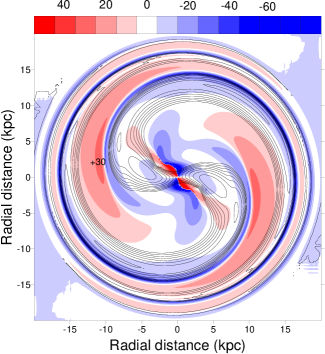
Figure 1: Positive stellar density perturbation superimposed on the vertex deviation map at $t=1.6$ Gyr. Positive and negative vertex deviations are shown in grey scale. The numbers indicate the maximum positive vertex deviation in the inter-arm region and maximum negative vertex deviation in the outer disk. The scale bar is in degrees. More details about this simulation as well as a color figure can be found in vorobyov08 , fig. 9.

We studied the evolution of an initially exponential disk which develop a two-armed spiral. Its vertex deviation shows a large spatial variation (Fig. 1). The values reach up to $90^{\circ}$ in the central region. A strong variation of $l_{\rm v}$ has been found at the outer edges of the spiral structures: $l_{\rm v}$ can vary there from $+40^{\circ}$ to $-40^{\circ}$ within only a few kpc. The epicyclic approximation fails almost everywhere with respect to the vertex deviation (or the Oort ratio). For more details, see Vorobyov & Theis vorobyov08 .

3 Test particle simulations

Our BEADS-2D code is based on the assumption of vanishing 3rd order velocity moments. In the case of pressure-supported stellar systems like globular clusters 3rd order terms are related to the heat flux which is controlled by two-body relaxation. Therefore, the zero-heat flux assumption (ZHFA) can be safely adopted on short timescales (e.g. a few dynamical timescales) due to long two-body relaxation timescales for stellar systems with more than $10^{4}$ stars. However, for rotation-supported systems like disk galaxies the situation is less clear. Still, the two-body relaxation time is long, but now large-scale motions might result in non-negligible higher order moments.

In order to study the ZHFA, we performed test particle simulations for a galactic disk. We measured the velocity moments up to fifth order at different galactocentric radii. Assuming a constant pattern speed $\Omega_{s}$ we solved for the equations of motion of a set of test particles in a corotating frame in polar coordinates,

$$\ddot{R} = R\phi-\frac{\partial\Phi}{\partial R}+2R\dot{\phi}\Omega_{s}+\Omega_{s}^{2}R,\hskip 22.76228pt\ddot{\phi}=-2\frac{\dot{R}}{R}\dot{\phi}-\frac{1}{R^{2}}\frac{\partial\Phi}{\partial\phi}-2\frac{\dot{R}}{R}\Omega_{s}\,.$$

$R$ and $\phi$ describe the radial and azimuthal coordinate of the particle’s trajectory, respectively. The gravitational potential $\Phi(\vec{r},t)$ at position $\vec{r}$ and time $t$ is split into two parts. The first part is a stationary, axisymmetric potential $\Phi_{0}(R)$ derived from a given rotation curve $v_{c}(R)$ with the galactocentric distance $R$. For a better comparison with other authors we chose the rotation curve suggested by Contopoulos & Grosbøl (cf. eq. (2) in contopoulos86 and parameters therein). The second part of the gravitational potential was selected to be a time-dependent (rigidly rotating) two-armed spiral perturbation also suggested in contopoulos86 :

$$\Phi(R,\phi)=f(t)\cdot ARe^{-\epsilon_{s}R}\cdot\cos(m\ln R/\tan i_{0}-2\phi)$$ (2)

For our model we adopted a two-armed ($m=2$) spiral with an amplitude $A=200\,\mathrm{km}^{2}\,\mathrm{s}^{-2}\,\mathrm{kpc}^{-1}$, an inverse scale length $\epsilon_{s}=0.1\,\mathrm{kpc}^{-1}$ and a pitch angle $i_{0}=-30^{\circ}$. We selected $\Omega_{s}=12.5\,\mathrm{km}\,\mathrm{s}^{-1}\,\mathrm{kpc}^{-1}$ which puts corotation (CR) at a radius of about 23 kpc, the 1/4-resonance (UHR) at 12 kpc and the inner Lindblad resonance at 1.4 kpc. In order to avoid any initial kicks the perturbation was switched-on ”adiabatically” on a timescale of 600 Myr. This procedure is attributed to the function $f(t)$ which we chose as in blitz91 .

For our statistical analysis we adopted an approach similar to that of Blitz & Spergel blitz91 . Initially $2\cdot 10^{6}$ stars were distributed in an exponential disk within a radial range from 4 to 40 kpc and a scale length of 10 kpc. The initial velocities were taken to be nearly circular (derived from the rotation curve) with a superimposed small perturbation: the radial velocity was derived from a Gaussian distribution with a dispersion of 20 km/s. The azimuthal velocity perturbation was calculated from a Gaussian distribution, taking asymmetric drift and the ratio of the radial to the azimuthal velocity dispersions within the epicyclic approximation into account blitz91 .

The velocity data are analysed on a polar grid ranging from 4 to 40 kpc with a radial grid spacing of 200 pc and an azimuthal spacing of 500 grid cells. Similar to blitz91 we measured the position of an orbit in intervals of $10^{6}$ years and considered its contribution to the velocity moments of this cell. By this technique (which is based on the ergodicity assumption), a single orbit yields many contributions to the velocity moments, by this strongly increasing the sample size. E.g. a subset of about $2.3\cdot 10^{5}$ particles hitting the radial range of 11.9 to 12.1 kpc yields about $3\cdot 10^{7}$ contributions to the velocity moments in this annulus (measured within the last 2 Gyr of the simulation). In order to be able to detect evolutionary effects, we sampled usually the orbits in 10 different periods with a duration of 1 Gyr each.

4 Results

During the simulations we calculated the cumulative velocity moments $v_{r}^{v}v_{\phi}^{w}$ for each cell hit by a particle and for all sums $s=v+w$ of the exponents ranging from $s=0$ up to $s=5$. From the corresponding mean velocity moments we derived the corresponding velocity dispersion terms including higher order terms $\sigma_{ijk},\sigma_{ijkl}$ and $\sigma_{ijklm}$ with $i,j,k,l,m=r\,\mathrm{or}\,\phi$ like $\sigma_{rrr}\equiv\overline{\left(v_{r}-u_{r}\right)\left(v_{r}-u_{r}\right)\left(v_{r}-u_{r}\right)}=\overline{v_{r}^{3}}-3\overline{v_{r}^{2}}u_{r}+2u_{r}^{3}$ (with the mean radial velocity $u_{r}\equiv\overline{v_{r}}$). We controlled our dispersion term calculation by Mathematica.

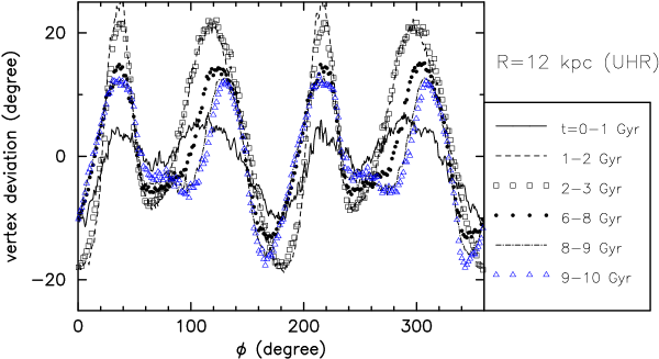
Figure 2: Azimuthal distribution of the vertex deviation $l_{\rm v}$ sampled at different times at a galactocentric distance of 12 kpc (UHR) in a annulus of 200 pc thickness.

Fig. 2 shows the azimuthal distribution of the vertex deviation near the UHR (1:4 resonance) at 12 kpc. Similarly to our BEADS-2D result a four armed-structure is visible for the vertex deviation. Already within the first Gyr four peaks are visible at about the final positions (a slight shift to larger angles can be seen for the second and the fourth peak). However, the absolute values of the vertex deviations vary considerably in time. It is interesting to note that the maximum values of $l_{\rm v}$ exceed the final values (at 10 Gyr) by about a factor of 2. After 6 Gyrs the final values are reached within 20%.

This strong temporal variation is a caveat for test particle simulations: obviously the stellar system needs a long time (by far longer than 3 Gyr) to reach an equilibrium configuration. However, in reality, perturbations evolve on shorter timescales: some might be growing, others might be vanishing. Therefore matching absolute values derived from equilibrium configurations of test particle simulations to observational values can be misleading, because the stellar system might not have the time to establish an equilibrium. The latter strongly favors either self-consistent simulations (like the BEADS-2D approach) or non-equilibrium analyses of test particle models.

The applicability of the BEADS-2D models depends on the validity of the zero-heat flux approximation. Therefore, we calculated the third (and higher) order terms all over the disk. At the UHR most of the third order terms show a clear, well-defined fourfold structure characteristic for the 1:4 resonance region (e.g. patsis06 ). Compared to the initial velocity dispersion (2nd order term) of 20 km/s, most (normalized) values of the 3rd order terms are smaller, but not necessarily negligible.

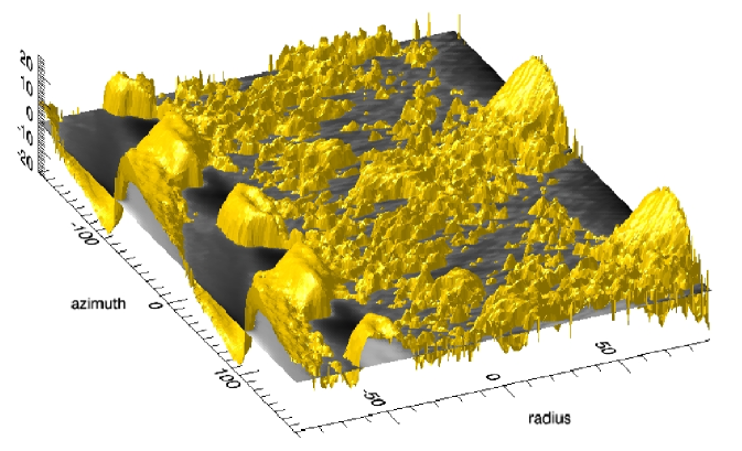
Figure 3: Distribution of the normalized third order velocity dispersion term $\mathrm{sign}(\sigma_{rrr})\cdot\left(|\sigma_{rrr}|\right)^{1/3}$ in the galactic disks sampled in the period 9-10 Gyr. Both axes denote the indices of the corresponding polar coordinates. The radial index 0 corresponds to the corotation radius (23 kpc), whereas the index -90 denotes the inner edge of the disk (4 kpc). The UHR is at about -50. The $z$-axis is given in km/s; For better visualisation the data have been smoothed and filtered.

A view over the whole disk, however, shows that the third order terms are especially large at the UHR and become negligible elsewhere. E.g. Fig. 3 displays $\sigma_{rrr}$ exhibiting clearly the four peaks associated with the 1:4 resonance. Beyond the UHR there are no significant third order terms discernible; it just looks like noise. Although one might speculate that some small structure can be identified by the broader “hills” at corotation, it is remarkable that corotation does not exhibit a more pronounced third order term. The strong peaks found at the lower and higher radial range are due to incomplete sampling: e.g. we did not consider stars inside 4 kpc which gives a bias in the velocity distribution near the inner edge.

It is also interesting to look for terms higher than third order. Near the UHR some of them become very large. E.g. $\sigma_{rr\phi\phi}$ reachs (normalized) peak values of 70 km/s and never drops below 20 km/s. Though other terms are smaller, they all are of the order of the initial velocity dispersion of the stars. Thus, there is no strong decay in magnitude for the higher order velocity dispersion terms near the UHR.

5 Summary

We analysed the structure of the velocity space in galactic disks which are subject to a spiral perturbation. In previous papers we used the Boltzmann moment equations up to second order in order to study the growth and saturation of spiral structure in self-gravitating stellar disks. From this analysis we derived the properties of the velocity ellipsoid all over the disk, namely the vertex deviations and the Oort ratios.

A key assumption of the BME approach is the zero-heat flux approximation, i.e. the neglection of third order velocity terms. We tested this assumption by performing test particle simulations for stars in a disk galaxy subject to a rotating spiral perturbation. As a result we corroborated qualitatively the complex velocity structure found in the BME approach. It turned out that an equilibrium configuration in velocity space is only slowly established on a typical timescale of 5 Gyrs or more. Since many dynamical processes in galaxies (like the growth of spirals or bars) act on shorter timescales, pure equilibrium models might not be fully appropriate for a detailed comparison with observations like the local Galactic velocity distribution. In our simulations third order velocity moments were typically small and uncorrelated over almost all of the disk with the exception of the 1:4 resonance region (UHR). Near the UHR (normalized) fourth and fifth order velocity moments are still of the same order as the second and third order terms. Thus, at the UHR higher order terms are not negligible.

Acknowledgements. CT is very grateful to the organizers of the meeting for a very interesting and inspiring conference as well as for the financial support. Additionally, we would like to thank Christoph Lhotka for his advice in using Mathematica.

References

- (1) Alcobé S., Cubarsi R., 2005, A&A, 442, 929
- (2) Bienaymé O., 1999, A&A, 341, 86
- (3) Binney J., Merrifield M. S., 1998, Galactic Astronomy, Princeton Univ. Press
- (4) Blitz L., Spergel D.N., 1991, ApJ, 370, 205
- (5) Contopoulos G., Grosbøl P., 1986, A&A, 155, 11
- (6) Dehnen W., 1998, AJ, 115, 2384
- (7) Dehnen W., 2000, ApJ, 119, 800
- (8) Dehnen W., Binney J.J., 1998, MNRAS, 298, 387
- (9) Eddington A.S., 1906, MNRAS, 67, 34
- (10) ESA, 1997, The Hipparcos and Tycho Catalogues (ESA Sp-1200)
- (11) Hogg D.W., Blanton M.R., Roweis S.T., Johnston K.V., ApJ, 629, 268
- (12) Kapteyn J.C., 1905, Rep. of the Brit. Ass. for the Advanc. of Science, p. 257
- (13) Kobold H., 1890, Astron. Nachr. 125, 65
- (14) Kuijken K., Tremaine S., 1991, in Proc. of Dynamics of Disc Galaxies, Göteborg, B. Sundelius (ed.), p. 71
- (15) Mayor M., 1970, A&A, 6, 60
- (16) Mayor M., 1972, A&A, 18, 97
- (17) Minchev I., Quillen A.C., 2007, MNRAS, 377, 1163
- (18) Minchev I., Nordhaus J., Quillen A.C., 2007, ApJ, 664, L31
- (19) Mühlbauer G., Dehnen W., 2003, A&A, 401, 975
- (20) Patsis P., 2006, MNRAS, 369, L56
- (21) Press W.H., Teukolsky S.A., Vetterling W.T., Flannery B.P., Numerical Recipes, 1992, Cambridge Univ. Press
- (22) Ratnatunga K.A., Upgren A.R., 1997, ApJ, 476, 811
- (23) Schwarzschild K., 1907, Nachr. Kgl. Ges. d. Wiss. zu Göttingen, Math. Phys. Klasse, 5, 614
- (24) Vorobyov E.I., Theis Ch., 2006, MNRAS, 373, 197 (VT06)
- (25) Vorobyov E.I., Theis Ch., 2008, MNRAS, in press, cf. also astro-ph/0709.2768
- (26) Wielen R., 1974, Highlights of Astronomy, 3, 395
- (27) Yuan C., 1971, AJ, 76, 664