Direct measurement of the cross-shock electric potential at low plasma $\beta$, quasi-perpendicular bow shocks

Abstract

We use the Cluster EFW experiment to measure the cross-shock electric field at ten low $\beta$, quasi-perpendicular supercritical bow shock crossings on March 31, 2001. The electric field data are Lorentz-tranformed to a Normal Incidence frame (NIF), in which the incoming solar wind velocity is aligned with the shock normal. In a boundary normal coordinate system, the cross-shock (normal) electric field is integrated to obtain the cross shock potential. Using this technique, we measure the cross-shock potential at each of the four Cluster satellites and using an electric field profile averaged between the four satellites. Typical values are in the range 500-2500 volts. The cross-shock potential measurements are compared with the ion kinetic energy change across the shock. The cross-shock potential is measured to be from 23 to 236% of the ion energy change, with large variations between the four Cluster spacecraft at the same shock. These results indicate that solar wind flow through the shock is likely to be variable in time and space and resulting structure of the shock is therefore nonstationary.

Submitted to Geophysical Research Letters, BALE ET AL. NIF Electric potential at shocks Stuart D. Bale, Space Sciences Laboratory, University of California, Berkeley, CA 94720-7450, USA. (bale@ssl.berkeley.edu)

1 Introduction

At collisionless shocks, a large ’cross-shock’ electric potential arises to oppose the incoming plasma flow. This potential, and its corresponding electric field, have the sense to repel incoming ions (which comprise the bulk of the kinetic energy and momentum) and to reflect some ions, providing additional dissipation and also plays a role in the redistribution of the upstream flow and magnetic field to the downstream state; the physics of this energy partitioning is not yet fully understood.

In the Ohm’s law sense, the cross-shock electric field arises from a combination of the Hall current, electron pressure gradients, and drag due to the small population of gyrating ions at the shock front. There are few, reliable published measurements of the cross-shock potential, largely because it requires a DC (double-probe) electric field instrument and these have been deployed primarily on low-apogee magnetospheric missions. Formisano [1982] estimated a voltage drop of 140 and 240V at two shocks. The double-probe instrument on ISEE was used to measure electric fields of up to 100 mV/m at the shock [Wygant et al., 1987] and a Normal Incidence Frame (NIF) electric potential of 420V [Scudder et al., 1986]. Eastwood et al. [2007] used Cluster measurements to calculate a potential drop of 260V, which corresponded to the ion kinetic energy change across the shock. Very large electric fields (600 mV/m), including parallel electric fields of 100 mV/m have been measured by the Polar spacecraft at a high Mach shock [Bale and Mozer, 2007], however the single-spacecraft Polar mission does not allow for good estimates of shock frame transformations. Furthermore, the bow shock is known to have large amplitude electric field structure from electron inertial scales [Walker et al., 2004] down to Debye scales [Bale et al., 1998]. Several authors have used a Liouville mapping of thermal electrons across the bow shock to estimate the deHoffman-Teller frame shock potential [viz. Schwartz et al., 1988], which can be related back to the NIF potential by a frame transformation. Gedalin [1997] calculated the expected shock potential (assuming pressure balance) and found that it should peak at an Alfven Mach number of around 2; this is where the magnetic compression begins to saturate, while the shock thickness continues to grow [Bale et al., 2003] with Mach numbers, leading to a small potential and more magnetic reflection at high Mach numbers.

The four Cluster spacecraft can be used to calculate a shock reference frame, which is important to transform correctly electric field data. In this letter, we measure directly the cross-shock electric field and compute the NIF electric potential. We find that the potential varies significantly between the different spacecraft at the same shock, indicating rapid temporal and/or spatial variations. This seems to be consistent with expectations of shock ’reformation’ [e.g. Krasnoselskikh et al., 2002; Hellinger et al., 2002 Matsukiyo and Scholer, 2006] and indicates that plasma flow through the shock and particle heating and energization are likely to be bursty.

2 Cluster data

The four Cluster spacecraft fly together in a controlled tetrahedron orbit with apogee near 19 $R_{e}$ and inter-spacecraft separations that vary from a few hundred to several thousand kilometers. Each winter, apogee passes through the dayside of the magnetosphere and Cluster crosses the bow shock (at least twice during each 57 hour orbit). On March 31, 2001, Cluster encountered the bow shock 11 times as a CME/magnetic cloud passed over the earth. The large, steady magnetic field of the cloud gives a low upstream plasma $\beta$ and hence, very planar bow shocks, which are ideal for this study. The alpha particle density was especially high during this interval, with an average value of $n_{\alpha}/n_{p}\approx 9\%$, as is often the case within magnetic clouds. The alpha density was used in computing ion masses below; however, it is not clear how the enhanced alpha density will effect the measured electric potentials.

The EFW experiment [Gustafsson et al., 1997] measures probe-to-spacecraft voltage on four 8 cm spherical voltage probes, each extended on wire booms 44 m from the spacecraft body, in the spin plane. Since only two components of the electric field are measured, we assume that $\vec{E}\cdot\vec{B}$ = 0 (ideal MHD) in order to determine the three-component electric field and correct this where required later. Since the $B_{z}$ (GSE) component is large here (in a CME), this makes for a good reconstruction of the missing ($E_{z}$) component of the electric field. The electric field data are calibrated locally near each shock by forcing agreement between the component of the ion velocity perpendicular to $\vec{B}$ and $(\vec{E}\times\vec{B})/B^{2}$; this correction is of order 1 mV/m in the $X$ GSE direction and minimizes any offsets due to varying plasma or photoelectron/secondary electron conditions. The sum of the four probe voltages gives an estimate of the spacecraft floating potential which is related functionally to the ambient plasma density. We fit the spacecraft potential locally (near each shock) to the plasma density to produce a high time resolution ’density proxy’ measurement. We also use magnetic field data from the FGM experiment [Balogh et al., 1997], ion moments from the CIS instrument [Reme et al., 1997], and electron temperatures from the PEACE instrument [Johnstone et al., 1997]. The fractional alpha particle density is estimated using ACE data upstream and convected back to the shock crossing time; the alpha density is used to estimate the solar wind mass density, where needed.

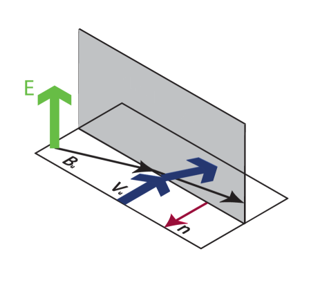
Figure 1: The shock coordinate system is defined with respect to the normal and the coplanarity plane, which contains the magnetic field and velocity vectors. In the normal incidence frame, the solar wind velocity is directed along the normal (red arrow). The convection electric field $\vec{E}=-\vec{v}\times\vec{B}$ (green arrow) is normal to the coplanarity plane and is approximately constant through the shock layer.

3 Measurements at bow shock crossings

Of the 11 bow shock crossings observed by Cluster on March 31, 2001, ten (10) of them were chosen for this study. These shocks were used by Maksimovic et al. [2003] to study global shock motion.

3.1 Shock normals

We compute the shock normal $\hat{n}$ by comparing the shock arrival time at the four Cluster satellites $\tau_{i}$ and inverting the matrix equation $\mathbf{r}\cdot\hat{n}=v_{sh}\vec{\tau}$, where $\mathbf{r}$ is a matrix of relative spacecraft positions and $v_{sh}$ is the shock speed in the spacecraft frame [viz Bale et al., 2003]. We do this separately using both spacecraft potential and magnetic field magnitude data and find normals that agree to within a few degrees and speeds that agree to within a few km/s, typically. Minimum variance normals are also in good agreement. A single spacecraft crosses the shock in 2-10 seconds typically and the shock transit time between different spacecraft is from 7 to 37 seconds.

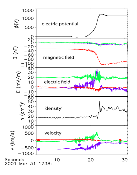
Figure 2: A typical shock crossing on March 31, 2001. The electric and magnetic fields and perpendicular velocity are in the coordinate system described in Figure 1; the purple line is the $\hat{x}$ component, green is $\hat{y}$, and red is the $\hat{z}$ component, large dots in the bottom panel show the perpendicular component of the ion velocity measured by CIS. The electric potential (top panel) is computed by integrating the normal (purple) component of the electric field (middle panel). The $B_{y}$ (out-of-coplanarity) magnetic field can be seen in the second panel (green trace).

3.2 Lorentz frame and coordinate transformations

The spacecraft-frame (measured) electric field can differ from that of the shock frame by several mV/m. Therefore, we Lorentz transform the measured field into the shock frame using the measured shock velocity $\vec{v}_{sh}=v_{sh}\hat{n}$ to generate the shock-frame electric field $\vec{E}_{sh}=\vec{E}+\vec{v}_{sh}\times\vec{B}$. Then we compute the NIF velocity $\vec{v_{NIF}}=\hat{n}\times(\vec{v}_{u}\times\hat{n})$, where $\vec{v}_{u}$ is the solar wind velocity in the shock frame, and Lorentz transform the electric field $\vec{E}_{NIF}=\vec{E}_{sh}+\vec{v}_{NIF}\times\vec{B}$ and the incoming flow velocity $v_{sw}=v_{u}-v_{NIF}$ to the NI frame. Note that to this point, we have assumed that $\vec{E}\cdot\vec{B}=0$ (which is a Lorentz invariant).

Finally, the shock frame electric and magnetic fields and velocity are rotated into a coordinate system (Figure 1) which is defined with the shock normal as the $\hat{x}$ direction and the maximum variance of the magnetic field vector as the $\hat{z}$ direction; $\hat{x}$ and $\hat{z}$ define the coplanarity plane. In this coordinate system, the cross-shock electric field is in the $\hat{x}$ direction, the convection electric field $-\vec{v}_{sw}\times\vec{B}$ is in the $\hat{y}$ direction, and the magnetic field shearing direction is $\hat{z}$. Figure 2 shows data in this frame and coordinate system at one of our shock crossings.

3.3 The cross-shock electric potential

The shock speed calculated as described in Section 3.1 is used to generate a spatial shock profile $dx=v_{sh}dt$ and the cross-shock ($\hat{x}$ component) electric field can be integrated directly to obtain the cross-shock potential. To compensate for the assumption of $\vec{E}\cdot\hat{B}=0$, we now assume that the true cross-shock electric field lies purely in the $\hat{x}$ (normal) direction, and that we are measuring only the projection of it perpendicular to $\hat{B}$; therefore the cross-shock field can be written as $\vec{E}_{s}=E_{s}~{}\hat{x}={\underline{(E_{s}\sin\Theta_{bn}})}\hat{\perp}-(E_{s}\cos\Theta_{bn})\hat{\parallel}$, where $\hat{\parallel}$ and $\hat{\perp}$ are unit vectors parallel and perpendicular to the magnetic field (and hence in the coplanarity plane). The perpendicular component (underlined above) is the measured $E_{\perp,x}$ and therefore we can recover the cross-shock field amplitude as $E_{s}=E_{\perp,x}/\sin\Theta_{bn}$ and this is the field that we integrate to obtain the NIF potential; this represent a correction of from $0.1\%$ for $\Theta_{bn}\approx 87^{\circ}$ to $21\%$ for $\Theta_{bn}\approx 56^{\circ}$ (see Table 1). It is interesting to note that the cross-shock electric field is comprised of both a large-scale DC field and shorter wavelength, spiky structures of comparable amplitude (viz [Walker et al., 2004]). These structures are included in the integral of cross-shock potential, however, the resulting potential profile is relatively smooth and monotonic (until the magnetic overshoot, which is mimicked in the electric potential profile).

At each shock, the electric potential $\phi_{SCi}$ is computed, as described above, on ${\it each}$ of the four Cluster spacecraft ($i=1,4$) and an ’average’ potential $\phi_{A}$ is computed by first aligning (in time) the data from the four spacecraft, computing an average cross-shock electric field profile, and then integrating it, so that $\phi_{A}$ is like a potential of the volume-averaged field. Table 1 lists the 10 shocks, their macroscopic parameters, the Alfven Mach number $M_{A}$, electron and proton plasma beta, the shock tangent angle $\Theta_{bn}$, and the ion energy $E=1/2mv^{2}_{u}$ and its change across the shock $\Delta E=1/2~{}m(v_{u}^{2}-v_{d}^{2})$, along with the measured electric potentials.

Table 1: Normal Incidence Frame (NIF) shock parameters and measured cross-shock electric potentials on March 31, 2001.

							cross-shock potential (volts)
Shock Time	$M_{A}$	$\beta_{e}$	$\beta_{p}$	$\Theta_{bn}$	E (eV)a	$\Delta$E (eV)b	$\phi_{SC1}$	$\phi_{SC2}$	$\phi_{SC3}$	$\phi_{SC4}$	${\phi_{A}}$c	${{\phi_{A}}}/{E}$	${{\phi_{A}}}/{\Delta E}$
17:14:45	2.4	0.03	0.02	83∘	2299	1926age	1973	1900th	2057	3245age	2190	0.95	1.14
17:18:50	2.9	0.01	0.01	85∘	2223	2116age	1200	830th	1754	1232age	1223	0.55	0.58
17:36:47	3.2	0.06	0.05	86∘	2458	2110age	251	535th	825	755age	482	0.20	0.23
17:38:20	3.9	0.05	0.06	86∘	2561	2331age	840	1884th	923	1375age	1239	0.48	0.53
18:02:15	3.4	0.03	0.03	87∘	2818	2467age	893	714th	1126	971age	909	0.32	0.37
18:28:40	5.5	0.10	0.10	84∘	2487	2266age	2373	1541th	1185	2348age	1800	0.72	0.79
18:48:20	2.5	0.11	0.07	57∘	2581	2121age	1748	1127th	920	1146age	1039	0.40	0.49
19:00:41	3.7	0.10	0.09	64∘	2362	2053age	2968	2813th	3623	2992age	2791	1.18	1.36
19:46:37	2.6	0.02	0.02	62∘	2261	1798age	1012	809th	726	980age	799	0.35	0.44
21:34:06	2.7	0.03	0.03	56∘	1820	1688age	4303	4987th	3495	5402age	3992	2.19	2.36

a$E=1/2mv^{2}_{u}$ is the NIF upstream ion kinetic energy b$\Delta E=1/2m(v^{2}_{u}-v^{2}_{d})$ is the NIF ion kinetic energy change from upstream to downstream cNote that ${\phi_{A}}$ is not the average of the four potentials, rather it is the cross-shock potential of the average shock electric field profile.

4 Discussion

The last columns of Table 1 show $\phi_{A}/E$ and $\phi_{A}/\Delta E$, the average cross-shock potential normalized to the upstream ion kinetic energy $E=1/2mv^{2}_{u}$ and its change across the shock $\Delta E=1/2m(v_{u}^{2}-v_{d}^{2})$. This is a measure of the ability of the shock to oppose the directed plasma flow; i.e. when the electric potential $\phi_{A}$ approaches the upstream ion energy $E$ the shock should turn back the entire solar wind thermal ion population. Figure 3 shows $\phi/E$ with the black dots as $\phi_{A}$ and the error bars representing the maximum and minimum $\phi_{i}$ at each shock and plotted against Alfven Mach number; red dots show the values of $\phi_{A}/\Delta E$ The electric potential can vary by nearly $100\%$ in some cases and in three of the ten cases, $\phi_{A}/E$ is greater than 1.

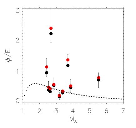
Figure 3: The cross-shock potential normalized to the upstream NIF ion kinetic energy $E=\phi/(1/2mv_{u}^{2})$ plotted against Alfvén Mach number. The black dots are computed from the ’average’ shock potentials $\phi_{A}$ and the error bars show the range of potential variation between the 4 Cluster satellites. Red dots show the ratio of $\phi_{A}$ to the NIF ion kinetic energy change $\Delta E=1/2m(v_{u}^{2}-v_{d}^{2})$. The dotted line is the analytical relationship from Gedalin (1997).

Gedalin [1997] estimated the cross-shock potential in the NIF analytically (assuming a monotonic shock profile and pressure balance) and found that the cross-shock potential peaks at small Alfven Mach numbers ($M_{A}\approx$ 2), qualitatively in agreement with dHT potentials inferred from Liouville mapping of thermal electrons [Schwartz et al.,, 1988]. Our NIF potentials show a similar trend (Figure 3), albeit with poor statistics; the dHT and NIF cross-shock ($\hat{x}$) electric fields are related by a frame transformation $E_{dHT}=E_{NIF}+(E_{y}/B_{x})B_{y}$.

Theoretical studies of shock reformation or nonstationarity predict that quasiperpendicular shock fronts should be unstable in certain regimes of Mach number and plasma $\beta$ [e.g. Krasnoselskikh et al, 2002; Hellinger et al., 2002; Matsukiyo and Scholer, 2006]. In particular, the constraint that the incoming solar wind speed be larger than the whistler phase speed and/or the ion thermal speeds allows the development of a shock front instability that results in ’overturning’ of the front with a characteristic timescale of the ion gyroperiod and a spatial scale of the ion gyroradius.

Recently Lobzin et al. [2007], using Cluster observations, provided convincing evidence that high Mach number quasiperpendicular shocks are nonstationary, moreover, a quasi-periodic shock front reformation takes place which modulates the reflected ion population.

In the reformation scenario, the shock electric potential will oscillate to large values on timescales of the ion gyroperiod $\tau_{ci}$. The time between shock crossings here (from spacecraft to spacecraft) ranges from 7 to 30 seconds, while the ion cyclotron period is $\tau_{ci}\approx$ 2 s; so it is plausible that these shocks are reforming rapidly and the four Cluster spacecraft each encounter the same shock at a different phase of the reformation cycle resulting in large variations in the measured potential. This strongly varying electric potential should produce a modulated reflected ion flux, as observed by Lobzin et al. [2007]. During this interval, the Cluster spacecraft were separated by 400-900 km, while $\rho_{i}\approx$ 200 km, so that the spacecraft-to-spacecraft variations may be spatial, rather than temporal.

This is the first multi-spacecraft study of the cross-shock electric potential (to our knowledge) and it shows that shock electric potentials vary largely on the timescale of the ion gyroperiod and/or spatial scales of ion gyroradii and that the Normal Incidence frame potential is often observed to be greater than the ion kinetic energy change across the shock. These observations are consistent with the quasiperpendicular shock reformation scenario and suggest that the transmission and reflection at the shock front are a bursty phenomena. This shock reformation may be due to an inherent instability (as described in references above) or due to solar wind driving, although there is no one-to-one signature of this in the upstream data [Maksimovic et al., 2003].