Particle current in a symmetric exclusion process with time-dependent hopping rates

Abstract

In a recent study (Jain et al 2007 Phys. Rev. Lett. 99 190601), a symmetric exclusion process with time-dependent hopping rates was introduced. Using simulations and a perturbation theory, it was shown that if the hopping rates at two neighboring sites of a closed ring vary periodically in time and have a relative phase difference, there is a net $DC$ current which decreases inversely with the system size. In this work, we simplify and generalize our earlier treatment. We study a model where hopping rates at all sites vary periodically in time, and show that for certain choices of relative phases, a $DC$ current of order unity can be obtained. Our results are obtained using a perturbation theory in the amplitude of the time-dependent part of the hopping rate. We also present results obtained in a sudden approximation that assumes large modulation frequency.

I introduction

The symmetric exclusion process (SEP) is one of the simplest and well studied models of a stochastic interacting particle system. In this model which can be defined on a $d$-dimensional hypercubic lattice, particles move diffusively while satisfying the hard core constraint that two particles cannot be on the same site. A number of exact results have been obtained for this model, particularly in one dimension Liggett (1985); Zia ; Schütz (2000). If the model is defined on a ring and conserves the total density, the system obeys the equilibrium condition of detailed balance in the steady state and thus does not support any net current. A lot of attention has also been given to non-equilibrium steady states of driven SEP in which the particles can enter or leave the bulk at the boundaries. For this model, the time-dependent correlation functions Santos and Schütz (2001) and dynamical exponents have been obtained using the equivalence of the transition matrix ($W$-matrix) to the Heisenberg model Stinchcombe and Schütz (1995). Recently, large deviation functional and current fluctuations have also been calculated for the driven SEP Spohn (1983); Derrida et al. (2002, 2004). Experimentally it has been shown that SEP can be used to model the diffusion of colloidal particles in narrow pores Gupta et al. (1995); Hahn et al. (1996); Kukla et al. (1996); Wei et al. (2000); Chou (1998); Chou and Lohse (1999).

Motivated by studies on quantum pumps where oscillating voltages can drive electron current across a wire Thouless (1983); Buttiker:1994 ; Aleiner and Andreev (1998); Brouwer:98 ; Switkes et al. (1999); Altshuler and Glazman (1999); Sharma:01 ; Ahorny:02 ; Watson et al. (2003); Andrei:03 ; Leek:05 ; Strass:05 ; Sela:06 ; Diptiman:07 , we have recently shown that similar effect can occur in a SEP model in which the hopping rates at two neighbouring sites are chosen to vary periodically in time and with a relative phase difference Jain Marathe Dhar Chowdhuri (2007). Our results obtained using Monte-Carlo simulations and a second-order perturbative calculation in the amplitude $f_{1}$ of the time-dependent part of the hopping rate can be summarized as follows: (i) A $DC$ current $\bar{J}$ is obtained, which decays with system size $L$ as $\bar{J}\sim 1/L$. Correspondingly the time averaged density profile varies linearly in the bulk of the system. (ii) The DC current $\bar{J}$ depends sinusoidally on the phase difference between rates at two sites. (iii) The dependence of $\bar{J}$ on driving frequency $\omega$ shows a peak at a frequency $\omega^{*}$ with $\bar{J}\rightarrow 1/\omega$ as $\omega\rightarrow\infty$ and $\bar{J}\rightarrow\omega$ as $\omega\rightarrow 0$. The latter result means that a finite number of particles are circulated even in the adiabatic limit.

Classical pumping of particles and heat, in similar time-dependent stochastic models, has also been studied in Astumian:2001 ; marathe07 ; sinitsyn07 ; ohkubo08 and seen in experiments Astumian (2003). Systems exhibiting pumping effect have often been modeled as Brownian ratchets in which non-interacting particles move in an external periodic potential. As discussed in astumian02 , these pump models are similar to Brownian ratchets Reimann (2002) where non-interacting particles placed in spatially asymmetric potentials that vary periodically in time and acted upon by noise execute directed motion. Models of non-interacting particles moving in symmetric potentials have also been considered parrondo98 ; usmani02 and pumping demonstrated. However for the model studied by us, particle interactions seem necessary for the pumping effect . Our model differs from such models in that here we are dealing with a many body particle system with interactions. For such an extended system, as described in the following section, the $n$-point equation does not close and involves next order correlation functions also. Pumping effect has also been found in the steady state of a driven SEP with two species ($A$ and $B$) of particles in which both species have the same diffusion constant Brzank and Schütz (2007). In this case, although the total current $J_{A}+J_{B}$ due to both species obeys the Fick’s law, the current due to one of the species does not follow the density gradient. However the pumping mechanism is different from that in our model where it arises due to the time-dependent rates.

In this paper, we consider a generalization of our earlier model by allowing the rates at all the sites to be time-dependent with a relative phase difference between neighbouring sites. The model is treated analytically using two approximations: a perturbation theory in the time-dependent part of the driving, and an expansion in the large frequency limit to leading orders. The treatment in this paper considerably simplifies the earlier one given in Jain Marathe Dhar Chowdhuri (2007). The most interesting new result is that in the model with time-dependent rates at all sites, a current of order unity can be obtained even in the thermodynamic limit for certain choices of relative phase differences.

The paper is organized as follows. In section (II), the model is defined. In section (III) the details of the first perturbation theory (expansion in $f_{1}$) are given, and two special choices of hopping rates are discussed. The results obtained from a sudden approximation (expansion in $1/\omega)$) are given in section (IV). Finally we end with a discussion in section (V).

II Definition of Model

The model is defined on a ring with $L$ sites. A site $l=1,2,3,...L$ can be occupied by $n_{l}=0$ or $1$ particle and the system contains a total of $N=\rho L$ particles where $\rho$ is the total density. A particle at site $l$ hops to an empty site either on the left or right with equal rates given by:

$$u_{l} = f_{0}+f_{1}v_{l}$$

$${\rm where}~{}~{}v_{l} = \alpha_{l}\sin(\omega t+\phi_{l})=\nu_{l}e^{i\omega t}+\nu_{l}^{*}e^{-i\omega t}~{}.$$ (1)

Here the site-dependent complex amplitudes are defined by $\nu_{l}=\alpha_{l}~{}e^{i\phi_{l}}/2i$ with $\alpha_{l}$ real and $f_{1}$ is chosen such that all hopping rates are positive. We will discuss two particular choices for the hopping rates in detail. Our first choice corresponds to the case where the hopping rates are time-dependent at only two sites of the ring, and we get an average current which decays inversely with system size. In the second case, we choose time-dependent hopping rates at all sites and show that a finite current can be obtained even in the thermodynamic limit.

A configuration of the system can be specified by the set $\{n_{l}\}$, $l=1,2,...L$. Let us define ${\bf P}(t)$ as the probability vector in the configuration space, with elements $P(C,t)$ giving the probability of the system being in the configuration $C=\{n_{l}\}$ at time $t$. Then the stochastic dynamics of the many particle system is described by the master equation:

$$\frac{d{\bf P}(t)}{dt}={\bf W}(t)~{}{\bf P}(t)={\bf W_{0}}~{}{\bf P}(t)+{\bf W_{1}}(t)~{}{\bf P}(t)$$ (2)

where ${\bf W}$ is the transition matrix, which we have split into a time-independent and a time-dependent part. One can also consider the time-evolution equations for $m$-point equal-time correlation functions $C_{l_{1},l_{2},l_{3},....,l_{m}}(t)=\langle n_{l_{1}}...n_{l_{m}}\rangle=\sum_{\{n_{l}\}}n_{l_{1}}...n_{l_{m}}P(\{n_{l}\},t)$. Thus, for example, the density $\rho_{l}(t)=\langle n_{l}\rangle$ and the two-point correlation function $C_{l,m}(t)$ satisfy the following equations:

$$\frac{\partial\rho_{l}}{\partial t}\ +2u_{l}\rho_{l}-u_{l-1}\rho_{l-1}-u_{l+1}\rho_{l+1}=u_{l}(C_{l-1,l}+C_{l,l+1})-u_{l+1}C_{l,l+1}-u_{l-1}C_{l-1,l}$$

$$\frac{\partial C_{l,m}}{\partial t}\ +2(~{}u_{l}+u_{m}~{})C_{l,m}-u_{l-1}~{}C_{l-1,m}-u_{l+1}~{}C_{l+1,m}-u_{m-1}~{}C_{l,m-1}-u_{m+1}~{}C_{l,m+1}$$

$$= u_{l}~{}(~{}C_{l-1,l,m}+C_{l,l+1,m}~{})+u_{m}~{}(~{}C_{l,m-1,m}+C_{l,m,m+1}~{})-u_{l-1}~{}C_{l-1,l,m}-u_{l+1}~{}C_{l,l+1,m}$$

$$-u_{m-1}~{}C_{l,m-1,m}-u_{m+1}~{}C_{l,m,m+1},~{}~{}{\rm for}~{}~{}~{}|l-m|\neq 1$$

$$\frac{\partial C_{l,l+1}}{\partial t}\ +(~{}u_{l}+u_{l+1}~{})C_{l,l+1}-u_{l-1}~{}C_{l-1,l+1}-u_{l+2}~{}C_{l,l+2}$$

$$= u_{l}~{}~{}C_{l-1,l,m}+u_{l+1}~{}C_{l,l+1,l+2}~{}-u_{l-1}~{}C_{l-1,l,l+1}-u_{l+2}~{}C_{l,l+1,l+2}~{}.$$ (4)

From Floquet’s theorem jung93 , it follows that the long time state of the system (assumed to be unique) will be periodic in time, with period $T=2\pi/\omega$. Here we will be mainly interested in the $DC$ current ${\bar{J}}$ defined as

$$\bar{J}_{l}=\frac{1}{T}\ \int_{0}^{T}J_{l,l+1}(t)~{}dt,$$ (5)

where the current $J_{l,l+1}$ in a bond connecting sites $l$ and $l+1$ is given by

$$J_{l,l+1}=u_{l}(\rho_{l}-C_{l,l+1})-u_{l+1}(\rho_{l+1}-C_{l,l+1})$$ (6)

and the local density $\rho_{l}=\langle n_{l}\rangle$. From the periodicity of the state at long times and particle conservation, it follows that the $DC$ current is uniform in space and therefore, using Eq. (6), we can write for the $DC$ current:

$$\bar{J} = \frac{1}{LT}\int_{0}^{T}\sum_{l=1}^{L}J_{l,l+1}(t)~{}dt$$ (7)

$$= \frac{f_{1}}{LT}\int_{0}^{T}\sum_{l=1}^{L}(v_{l+1}(t)-v_{l}(t))C_{l,l+1}(t)~{}dt$$ (8)

Thus to find the $DC$ current, we need to compute the two-point correlation function $C_{l,l+1}(t)$. In this paper, we will develop two different perturbation schemes, valid for general $v_{l}$, and then apply them to some special choices of the rates $v_{l}$.

Note that for $f_{1}=0$, the above model reduces to the homogeneous SEP with periodic boundary conditions whose properties are known exactly. In this case the steady state is an equilibrium state which obeys detailed balance and hence the average current is zero (note that this result holds even when the rates $\{u_{l}\}$ are site-dependent, but time-independent). In the steady state, all configurations are equally probable i.e. $P(C)=1/{L\choose N}$ when $f_{1}=0$. Then one can show that the density and correlation functions for the homogeneous SEP are given by:

$$\rho_{l}^{(0)} = \rho=\frac{N}{L}\$$

$$C_{l_{1},l_{2}}^{(0)} = \rho\frac{(N-1)}{(L-1)}\$$

$$C_{l_{1},l_{2},l_{3},....,l_{m}}^{(0)} = {L-m\choose N-m}/{L\choose N}.$$ (9)

III Perturbation theory: expansion in $f_{1}$.

For $f_{1}\neq 0$, the knowledge of the exact steady state of homogeneous SEP enables us to set up a perturbation expansion in $f_{1}$ of various observables. We now describe this perturbation theory within which we calculate an expression for ${DC}$ current $\bar{J}$ in the bulk of the system. A similar perturbation technique was developed for a two-state system in astumian89 . We expand various quantities of interest with $f_{1}$ as the perturbation parameter about the homogeneous steady state corresponding to $f_{1}=0$. Thus we write

$$\rho_{l}(t) = \langle n_{l}(t)\rangle=\rho+\sum_{r=1}^{\infty}f_{1}^{r}\rho_{l}^{(r)}(t)$$ (10)

$$C_{l,m}(t) = \langle n_{l}(t)n_{m}(t)\rangle=C_{l,m}^{(0)}+\sum_{r=1}^{\infty}f_{1}^{r}C_{l,m}^{(r)}(t)~{},$$ (11)

and similar expressions for higher correlations. Plugging in Eq. (11) into Eq. (8), we find that the lowest order contribution to $\bar{J}$ is at ${\cal{O}}(f_{1}^{2})$ and given by:

$$\bar{J}^{(2)}=\frac{f_{1}^{2}}{T~{}L}~{}\int_{0}^{T}\sum_{l=1}^{L}(~{}v_{l}~{}-~{}v_{l+1}~{})~{}C_{l,l+1}^{(1)}~{}dt~{}.$$ (12)

To develop our perturbation theory and find two-point correlation function $C_{l,m}^{(1)}$, we start with the time evolution equation for density $\rho_{l}(t)$ which is given by Eq. (II). Plugging in the expansions in Eqs.(10) and (11), we get the following equation for the density $\rho_{l}^{(r)}$ at $r^{th}$ order:

$$\frac{\partial\rho_{l}^{(r)}}{\partial t}\ - f_{0}\Delta_{l}\rho_{l}^{(r)}+2v_{l}\rho_{l}^{(r-1)}-v_{l-1}\rho_{l-1}^{(r-1)}-v_{l+1}\rho_{l+1}^{(r-1)}$$ (13)

$$= v_{l}(C_{l-1,l}^{(r-1)}+C_{l,l+1}^{(r-1)})-v_{l-1}C_{l-1,l}^{(r-1)}-v_{l+1}C_{l,l+1}^{(r-1)},$$

where $\Delta_{l}g_{l}=g_{l+1}-2g_{l}+g_{l-1}$ defines the discrete Laplacian operator. Thus the density at $r^{th}$ order can be obtained in terms of density and two point correlation function at $(r-1)^{th}$ order. We check that at the zeroth order, we obtain the homogeneous SEP for which the density and all equal time correlations are given by Eq. (9). At first order, the above equation then gives:

$$\frac{\partial\rho_{l}^{(1)}}{\partial t}\ -f_{0}\Delta_{l}\rho_{l}^{(1)}=r_{0}\Delta_{l}v_{l},$$ (14)

where $r_{0}=\rho-C_{l,m}^{(0)}$. The solution for this equation is the sum of a homogeneous part which depends on initial conditions and a particular integral. At long times the homogeneous part vanishes while the particular integral has the following asymptotic form:

$$\rho_{l}^{(1)}(t)=A_{l}^{(1)}e^{i\omega t}+A_{l}^{*(1)}e^{-i\omega t}.$$ (15)

Substituting Eq. (15) in Eq. (14) we obtain the following equation for $\{A_{l}^{(1)}\}$:

$$(i\omega+2f_{0})A_{l}^{(1)}-f_{0}A_{l-1}^{(1)}-f_{0}A_{l+1}^{(1)}=r_{0}(\nu_{l+1}-2\nu_{l}+\nu_{l-1})~{}.$$ (16)

This can be written in matrix form as:

$${\hat{Z}}(\omega)~{}~{}{\bf A}=-r_{0}~{}{\hat{B}}~{}{\bf\Phi},$$ (17)

where

$$Z_{lm} = -f_{0}~{}\delta_{l,m+1}+(~{}i\omega+2f_{0}~{})~{}\delta_{l,m}-f_{0}~{}\delta_{l,m-1}$$

$$B_{lm} = -\delta_{l,m+1}+2~{}\delta_{l,m}-\delta_{l,m-1}$$

$${\bf A} = \{A_{1}^{(1)},A_{2}^{(1)},....,A_{L}^{(1)}\}^{T},{\bf\Phi}=\{\nu_{1},\nu_{2},....,\nu_{L}\}^{T},$$ (18)

and periodic boundary conditions are implicitly taken. The above equation can be solved for ${\bf A}$ and we get:

$${\bf A}=-{r_{0}}~{}{\hat{G}}(\omega)~{}{\hat{B}}~{}{\bf\Phi},$$ (19)

where ${\hat{G}}(\omega)={\hat{Z}^{-1}}(\omega)$. Both ${\hat{G}}(\omega)$ and ${\hat{B}}$ are cyclic matrices and so can be diagonalized simultaneously. The eigenvalues of ${\hat{Z}}(\omega)$ are $i\omega+4f_{0}\sin^{2}(p\pi/L)$, while that of ${\hat{B}}$ are $4\sin^{2}(p\pi/L)$ with $p=1,2,...,L$, and eigenvector elements are $e^{i2\pi pl/L}/L^{1/2}$. Hence $A_{l}^{(1)}$ can be written as:

$$A_{l}^{(1)}=-\frac{4r_{0}}{L}\ \sum_{m=1}^{L}\sum_{p=1}^{L}~{}~{}\frac{e^{-i\frac{2\pi p(l-m)}{L}}~{}\sin^{2}(p\pi/L)~{}}{i\omega+4f_{0}\sin^{2}(p\pi/L)}\ \nu_{m},$$ (20)

which in the large $L$ limit gives:

$$A_{l}^{(1)}=-\frac{r_{0}}{f_{0}}\ \nu_{l}~{}+~{}\frac{ir_{0}\omega}{f_{0}^{2}}\ \frac{1}{z_{+}-z_{-}}\sum_{m=1}^{L}~{}[~{}z_{-}^{|m-l|}~{}+~{}z_{-}^{L-{|m-l|}}~{}]~{}\nu_{m},$$ (21)

where, $z_{-}=y/2-[(y/2)^{2}-1]^{1/2},~{}z_{+}=1/z_{-}$ and $y=2+({i\omega}/{f_{0}})$.

To compute the ${\cal{O}}(f_{1}^{2})$ contribution to $\bar{J}$, we need to evaluate $C_{l,m}^{(1)}$, which we now proceed to obtain. Inserting the perturbation series in Eqs. (10) and (11) into Eq. (4) we get the following equation for the correlation $C_{l,m}^{(r)}$ at $r^{th}$ order for $|m-l|\neq 1$:

$$\frac{\partial C_{l,m}^{(r)}}{\partial t}\ - f_{0}~{}(~{}\Delta_{l}+\Delta_{m}~{})~{}C_{l,m}^{(r)}+2v_{l}~{}C_{l,m}^{(r-1)}-v_{l-1}~{}C_{l-1,m}^{(r-1)}-v_{l+1}~{}C_{l+1,m}^{(r-1)}$$

$$+ 2v_{m}~{}C_{l,m}^{(r-1)}-v_{m-1}~{}C_{l,m-1}^{(r-1)}-v_{m+1}~{}C_{l,m+1}^{(r-1)}$$

$$= v_{l}~{}(~{}C_{l-1,l,m}^{(r-1)}+C_{l,l+1,m}^{(r-1)}~{})+v_{m}~{}(~{}C_{l,m-1,m}^{(r-1)}+C_{l,m,m+1}^{(r-1)}~{})$$

$$- v_{l-1}~{}C_{l-1,l,m}^{(r-1)}-v_{l+1}~{}C_{l,l+1,m}^{(r-1)}-v_{m-1}~{}C_{l,m-1,m}^{(r-1)}-v_{m+1}~{}C_{l,m,m+1}^{(r-1)},$$

$${\rm while~{}for}~{}~{}~{}m=l+1:$$

$$\frac{\partial C_{l,l+1}^{(r)}}{\partial t}\ + f_{0}~{}(~{}2C_{l,l+1}^{(r)}-C_{l-1,l+1}^{(r)}-C_{l,l+2}^{(r)}~{})$$

$$= v_{l+2}~{}(~{}C_{l,l+2}^{(r-1)}~{}-~{}C_{l,l+1,l+2}^{(r-1)}~{})~{}+~{}v_{l-1}~{}(~{}C_{l-1,l+1}^{(r-1)}~{}-~{}C_{l-1,l,l+1}^{(r-1)}~{})$$

$$- ~{}v_{l}~{}(~{}C_{l,l+1}^{(r-1)}~{}-~{}C_{l-1,l,l+1}^{(r-1)}~{})~{}-~{}v_{l+1}~{}(~{}C_{l,l+1}^{(r-1)}~{}-~{}C_{l,l+1,l+2}^{(r-1)}~{}).$$ (22)

At first order we get:

$$\frac{\partial C_{l,m}^{(1)}}{\partial t}\ - f_{0}(\Delta_{l}+\Delta_{m})C_{l,m}^{(1)}=k_{0}(\Delta_{l}v_{l}+\Delta_{m}v_{m})~{},$$

$$\frac{\partial C_{l,l+1}^{(1)}}{\partial t} + f_{0}\left(2C_{l,l+1}^{(1)}-C_{l-1,l+1}^{(1)}-C_{l,l+2}^{(1)}\right)=k_{0}(v_{l-1}+v_{l+2}-v_{l}-v_{l+1}),$$ (23)

where $k_{0}=C_{l_{1},l_{2}}^{(0)}-C_{l_{1},l_{2},l_{3}}^{(0)}$ and these are known from Eq. (9). The computation of even the homogeneous solution of the above set of equations is in general a non-trivial task because of the form of the equations involving nearest neighbor indices and requires a Bethe ansatz or dynamic product ansatz Schütz (2000); Santos and Schütz (2001). However it turns out that the long time solution can still be found exactly and is given by:

$$C_{l,m}^{(1)}(t)=\frac{k_{0}}{r_{0}}[\rho_{l}^{(1)}(t)+\rho_{m}^{(1)}(t)]=A_{l,m}^{(1)}e^{i\omega t}+A_{l,m}^{*(1)}e^{-i\omega t}~{},$$ (24)

where $A_{l,m}^{(1)}=(k_{0}/r_{0})(A_{l}^{(1)}+A_{m}^{(1)})$. It is easily verified that this satisfies Eq. (23) for all $l,m$. To determine whether the system indeed has a product measure requires a more detailed analysis of the higher order terms in the perturbation series and higher correlations. We have verified that at least to first order in perturbation theory, all correlation functions in fact have the same structure as the two-point correlation function in Eq. (24).

We now plug the solution in Eq. (24) into Eq. (12) for the average current in the system and after some simplifications obtain:

$$\bar{J}^{(2)}=-\frac{f_{1}^{2}}{L}\ ~{}\frac{k_{0}}{r_{0}}~{}\sum_{l=1}^{L}~{}(~{}A_{l+1}^{*(1)}\nu_{l}~{}+~{}A_{l+1}^{(1)}\nu_{l}^{*}~{}-~{}A_{l}^{*(1)}\nu_{l+1}~{}-~{}A_{l}^{(1)}\nu_{l+1}^{*}~{})~{},$$ (25)

with $A_{l}^{(1)}$ given by Eq. (21). For any given choice of the rates $\nu_{l}$, this general expression can be used to explicitly evaluate the net $DC$ current in the system.

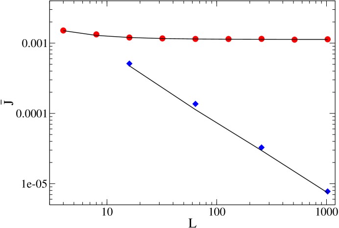
Figure 1: Log-log plot of $\bar{J}$ versus system size $L$ at half filling for two cases discussed in the text. The points (◆) correspond to simulations for the $2$ special sites problem with $\phi=\pi/2$, $f_{0}=0.3$, $f_{1}=0.2,~{}\omega=0.2\pi$. In this case the current goes as $\sim L^{-1}$. The points (⚫) corresponds to all sites having time-dependent hopping rates with $q=\pi/2$ and $f_{0}=0.5,~{}f_{1}=0.1,~{}\omega=0.2\pi$. In this case the current goes to a constant value at large $L$. The bold lines indicate the results from the perturbation theory.

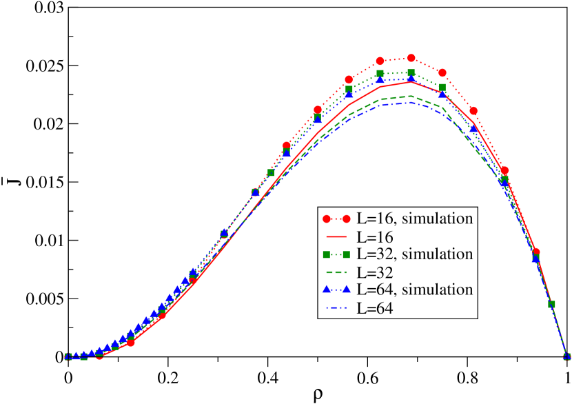
Figure 2: Plot of ${DC}$ current $\bar{J}$ versus density $\rho=N/L$ for parameters $f_{0}=0.5$, $f_{1}=0.4$, $\omega=0.2\pi$ and $\phi_{l}=\pi l/2$ for system sizes $L=16,32$ and $64$. Both the results from simulations (symbols connected by dotted lines) and from the perturbation theory (lines) are plotted.

We now consider two special choices of the rates $\{\nu_{l}\}$.

(i) The choice $\alpha_{1}=\alpha_{L}=1$, all other $\alpha_{l}=0$, and $\phi_{1}=0,\phi_{L}=\phi$ corresponds to the pumping problem with two special sites studied in Jain Marathe Dhar Chowdhuri (2007). In the limit of large $L$, this gives:

$${\bar{J}}^{(2)}=\left(\frac{f_{1}}{f_{0}}\right)^{2}\frac{k_{0}\omega\sin\phi}{L}~{}{\rm Re}[z_{-}],$$ (26)

which agrees with the result presented in Jain Marathe Dhar Chowdhuri (2007) ( apart from a factor of two which was missed in that paper). Writing $z_{+}=re^{i\eta}$, we find that for $\omega\ll\omega^{*}=2f_{0}$, the magnitude $r\approx 1+\sqrt{\omega/\omega^{*}}$ and the angle $\eta\approx\sqrt{\omega/\omega^{*}}$. In the opposite limit, $r\approx 2\omega/\omega^{*}$ and $\eta\approx\pi/2-\omega^{*}/\omega$. Using $z_{+}=1/z_{-}$, we find that the current has the scaling form:

$${\bar{J}}^{(2)}=\frac{f_{1}^{2}k_{0}\sin\phi}{f_{0}L}G\left(\frac{\omega}{2f_{0}}\right)$$ (27)

where the scaling function $G(x)=2x$ for $x\ll 1$ and $1/x$ for $x\gg 1$. We note that $\bar{J}$ is independent of $f_{0}$ for large $x$. This can be seen by writing the master equation as:

$$\frac{d{\bf P}}{d(\omega t)}=\frac{f_{0}}{\omega}{\bf W_{0}P(t)}+\frac{f_{1}}{\omega}{\bf W_{1}P(t)}~{}.$$ (28)

For $\omega\gg f_{0}$, the first term on the right hand side can be neglected thus giving the probability distribution to be a function of $f_{1}/\omega$.

(ii) The second case we consider here assumes $\alpha_{l}=1$ at all sites and $\phi_{l}=ql$, where $q=2\pi s/L$ with $s=1,2...L/2$, so that there is a constant phase difference $q$ between successive sites. In this case, $A_{l}^{(1)}$’s given by Eq. (20), evaluated at large $L$ gives:

$$A_{l}^{(1)} = \frac{ir_{0}}{2f_{0}}e^{iql}a$$ (29)

$${\rm where}~{}~{}a = \frac{1-\cos q}{y/2-\cos q}$$

and from Eq. (25) we get for the average current:

$$\bar{J}^{(2)} = -\frac{f_{1}^{2}k_{0}}{f_{0}}\sin q~{}{\rm Im}[a]~{}$$ (30)

$$= \frac{2~{}f_{1}^{2}~{}k_{0}~{}\omega~{}\sin q~{}(1-\cos q)}{[~{}\omega^{2}~{}+~{}4f_{0}^{2}~{}(1-\cos q)^{2}~{}]}\ .$$

Thus we see that for most values of $q$ we get a finite current, even in the limit $L\to\infty$. For $q\sim 1/L$ and $q\sim\pi-1/L$, the current goes to zero for large system size as $\bar{J}\sim L^{-3}$. From the current expression in Eq. (30), we can find out the value $q=q^{*}$, at which the current is a maximum. By differentiating Eq. (30) with respect to $q$ we get:

$$\cos(q^{*})=(1+\Omega^{2})-\sqrt{(1+\Omega^{2})^{2}-(1-\Omega^{2})},$$ (31)

where $\Omega=\omega/2f_{0}$. It turns out that for large $\omega$ the maximum is at $q^{*}=2\pi/3$, while for small frequencies we get $q^{*}\sim\sqrt{\omega}$. Also we find from Eq. (30) that in the adiabatic and fast drive limits, the currents are respectively given by:

$$\bar{J}^{(2)}=\begin{cases}\frac{f_{1}^{2}k_{0}}{2f_{0}^{2}}~{}{\cot(q/2)}~{}\omega~{}~{}~{},~{}~{}~{}\omega/f_{0}<<(1-\cos q)\\ 2f_{1}^{2}k_{0}\sin q(1-\cos q)~{}\frac{1}{\omega}~{}~{}~{},~{}~{}~{}\omega/f_{0}>>1~{}.\end{cases}$$ (32)

The perturbation theory results described above turn out to be quite accurate as can be seen from the comparisons with simulation results shown in Fig. (1) for both cases (i) and (ii). In this figure, we have plotted the current for different system sizes and verify the $\bar{J}\sim L^{-1}$ dependence for case (i) and $\bar{J}\sim L^{0}$ for case (ii) with $q=\pi/2$. Using the expression for $k_{0}$ in Eqs. (26, 30), we find that ${\bar{J}}^{(2)}\sim\rho^{2}(1-\rho)$ which has a maximum at $\rho^{*}=2/3$ and breaks particle-hole symmetry. This particle-hole asymmetry can be understood easily. From the definition of the model we see that, unlike the particles, the hopping rates of a hole are not symmetric: a hole at site $l$ hops towards right with rate $u_{l+1}$ and left with $u_{l-1}$. In Fig. (2) we have plotted simulation results for the average current as a function of particle density, for different system sizes, and find good agreement with our perturbative result, even at a relatively large value of $f_{1}/f_{0}$.

In simulations we have looked at the density profiles and find that the site wise density profile $\bar{\rho}_{l}$ in case (ii) is flat. This is unlike in Jain Marathe Dhar Chowdhuri (2007), where we found high densities at the two special sites and then a linear density profile in the bulk. The flat density profile, for case (ii), is understood because here there are no special pumping sites. It is interesting that we can get current in the system even in the absence of Fick’s law. We also note that even if the hop-out rates are made biased in one direction, like in the asymmetric exclusion process (ASEP), we can still get a current opposing this bias (for small biases).

IV Sudden approximation: $\omega/f_{0}\gg 1$

In this section, we find the $DC$ current within sudden approximation following the procedure of Reimann:1996 . Calling $\theta=\omega t$, the master equation Eq. (2) can be rewritten as

$$\frac{d{\bf P}(\theta)}{d\theta}=\frac{1}{\omega}\left[{\bf W_{0}}+{\bf W_{1}}(\theta)\right]{\bf P}(\theta)$$ (33)

which can be expanded in powers of $1/\omega$ by using ${\bf P}(\theta)=\sum_{n=0}^{\infty}\omega^{-n}{\bf P}_{s}^{(n)}(\theta)$ to give

$$\frac{d{\bf P}_{s}^{(0)}}{d\theta} = 0$$ (34)

$$\frac{d{\bf P}_{s}^{(1)}(\theta)}{d\theta}-{\bf W_{1}}(\theta){\bf P}^{(0)}_{s} = {\bf W_{0}}{\bf P}^{(0)}_{s}$$ (35)

and so on. From the zeroth order equation, we see that ${\bf P}^{(0)}_{s}$ is independent of $\theta$. In fact, for $\omega\to\infty$, we expect the system to behave as the unperturbed homogeneous SEP for which ${\bf W_{0}}{\bf P}^{(0)}_{s}=0$ is satisfied and as discussed in Section II, all the elements of the vector ${\bf P}^{(0)}_{s}$ are known. Using this fact, the first order correction ${\bf P}^{(1)}_{s}$ can be found by integrating Eq. (35) over $\theta$. Following steps as those leading to Eq. (12), we can obtain an expression for average current $\bar{J}_{s}$ at order ${\cal{O}}(1/\omega)$ which is given by:

$${\bar{J}}_{s}^{(1)}=\frac{f_{1}}{2\pi\omega L}\int_{0}^{2\pi}d\theta~{}\sum_{l=1}^{L}(v_{l+1}-v_{l}){\tilde{C}}_{l,l+1}^{(1)}$$ (36)

where we have expanded the nearest neighbor correlation function $C_{l,l+1}=\sum_{n=0}^{\infty}\omega^{-n}{\tilde{C}}_{l,l+1}^{(n)}$ in powers of $1/\omega$ and used the expression for ${\tilde{C}}_{l,l+1}^{(0)}=C_{l,l+1}^{(0)}$ given by Eq. (9). The first order correction to correlation function can be obtained by perturbatively expanding Eq. (4) and obeys the following simple equation:

$$\frac{d{\tilde{C}}^{(1)}_{l,l+1}}{d\theta}=f_{1}k_{0}~{}(v_{l+2}+v_{l-1}-v_{l}-v_{l+1})~{}.$$ (37)

We now again discuss the two special choices of rates $v_{l}$, discussed in the previous section.

(i) In this case, only two sites have time-dependent hopping rates. Solving the equations above for the correlation function, we get:

$${\tilde{C}}^{(1)}_{1,2} = f_{1}k_{0}(\cos(\theta)-\cos(\theta+\phi))+c_{1,2}$$ (38)

$${\tilde{C}}^{(1)}_{L-1,L} = -f_{1}k_{0}(\cos(\theta)-\cos(\theta+\phi))+c_{L-1,L}$$ (39)

$${\tilde{C}}^{(1)}_{L,1} = f_{1}k_{0}(\cos(\theta)+\cos(\theta+\phi))+c_{L,1}$$ (40)

where $c_{i,j}$ are constants of integration (which do not contribute to current). Using the above equations in the expression for ${\bar{J}}^{(1)}_{s}$, we finally obtain

$${\bar{J}}^{(1)}_{s}=\frac{2f_{1}^{2}k_{0}\sin\phi}{\omega L}~{}.$$ (41)

Thus, we find that to leading order in $1/\omega$ (and arbitrary $f_{1}$), the $DC$ current is the same as the one obtained by taking large $\omega$ limit in the current expression Eq. (27) obtained from the $f_{1}$ expansion.

(ii) In this case with $\alpha_{l}=1$ at all sites, the equations for the first order correlation functions can be solved for arbitrary phases $\phi_{l}$, and we get:

$${\tilde{C}}_{l,l+1}^{(1)}=k_{0}f_{1}\left[\cos(\theta+\phi_{l})+\cos(\theta+\phi_{l+1})-\cos(\theta+\phi_{l-1})\cos(\theta+\phi_{l+2})\right]~{}.$$ (42)

Using these in the current expression and after some simplifications, we get:

$${\bar{J}}_{s}^{(1)}=\frac{k_{0}f_{1}^{2}}{\omega L}\sum_{l=1}^{L}\left[2\sin(\phi_{l+1}-\phi_{l})-\sin(\phi_{l+1}-\phi_{l-1})\right].$$ (43)

Note that the above expression depends on the phase difference between nearest and next nearest neighbor sites. For $\phi_{l}=ql$, we recover the result stated in the second line of Eq. (32).

V Discussion

In this article, we have considered a lattice model of diffusing particles with hard core interactions and shown that if the hopping rates at various sites are chosen to be symmetric but time-dependent, a $DC$ current can be generated in the system. Thus a ratchet effect is obtained in the sense that a directed current occurs even though there is no net applied external biasing force. Unlike many other examples of models of classical ratchets, there is no asymmetric potential or asymmetric noise in our model. However asymmetry is incorporated in the modulation of the hopping rates, and this is best seen when we consider the case where the modulation is given by $v_{l}(t)=\sin(\omega t-ql)$. This of course corresponds to a wave traveling in a given direction. A non-trivial aspect of the problem studied is the fact that the effect goes away as soon as we switch off the hard-core interactions. For non-interacting particles, the $DC$ current given by ${\bar{J}}=({1}/{LT})\int_{0}^{T}dt~{}\sum_{l=1}^{L}u_{l}\rho_{l}-u_{l+1}\rho_{l+1}$, is immediately seen to be exactly zero for arbitrary choice of the time-dependent rates. On the other hand, having interactions in the system is not a sufficient condition to generate a $DC$ current. For the models considered in this paper, the hopping rate is site-wise symmetric. But if the hopping rates are symmetric bond-wise, i.e., the hop rate $u_{l,l+1}$ from site $l$ to $l+1$ is the same as that from $l+1$ to $l$, then the $DC$ current is zero for any choice of phases $\phi_{l}$. To see this, consider the density evolution equation obeyed by bond-wise symmetric SEP:

$$\frac{\partial\rho_{l}}{\partial t}=u_{l-1,l}(\rho_{l-1}-\rho_{l})+u_{l,l+1}(\rho_{l+1}-\rho_{l})$$ (44)

Unlike Eq. (II) for site-wise symmetric SEP, $\rho_{l}=\rho$ is a solution of the above equation for any choice of rates $u_{l}$. In fact, an inspection of the master equation shows that, even with a time-dependent ${\bf W}$-matrix, all configurations are equally likely, thus leading to zero current. Thus the exclusion process with bond-wise symmetric rates does not give the ratchet effect. It is not completely clear as to what are the necessary and sufficient conditions to get a directed current sinitsyn08 .

For the model considered here, since the equations for any $n$-point correlation function do not close, it does not seem simple to solve the model exactly. We have therefore studied the system analytically using a perturbation theory in the amplitude $f_{1}$ and the inverse frequency $1/\omega$. In this paper, we have been able to obtain the $DC$ current at order $f_{1}^{2}$ by solving the evolution equations for density and two point correlation function to order $f_{1}$. This is unlike our earlier solution in Jain Marathe Dhar Chowdhuri (2007) where the density was obtained to second order in $f_{1}$. Also, we have been able to obtain results for large driving frequency by solving the correlation function alone by such perturbative approaches. Comparing with simulations we find that the perturbative results turn out to be quite accurate.

We now briefly comment on the adiabatic limit, which has been much studied in the quantum context. In our case, from our perturbation theory result we see that, over one time period of the driving there is a finite particle transport, even in the adiabatic limit. Formally we can obtain an exact expression for the net particle transport. For this we start with the master equation ${\partial{\bf P}}/{\partial t}={\bf W}(t){\bf P}$. Let ${\bf P}^{(0)}(t)$ be the instantaneous equilibrium solution satisfying ${\bf W}(t){\bf P}^{(0)}=0$. Then, for slow rates $\omega$, ${\bf P}(t)$ will have the form ${\bf P}^{(0)}(t)+\omega{\bf P}^{(1)}(t)$ where the correction is given by: $\omega{\bf P}^{(1)}={\bf W}^{-1}~{}{\partial{\bf P}^{(0)}}/{\partial t}$ . The net particle transported across any bond in one time cycle, ${\cal{N}}$, can then be expressed as:

$${\cal{N}}=\int_{0}^{T}dt\sum_{C}J(C)P(C,t)=-\int_{0}^{2\pi}dx\sum_{C,C^{\prime}}J(C)\frac{\partial W^{-1}_{C,C^{\prime}}(x)}{\partial x}P^{(0)}(C^{\prime},x)~{},$$ (45)

where $J$ refers to the current on any given bond. Thus we have a formal expression, for the net particle transported, in terms of an integral over an equilibrium average of some quantity. However this expression does not appear to have any simple physical interpretation and it is not easy to obtain any explicit results, unlike the fast case treated in section (IV). Recently adiabatic pumping phenomena have been studied in the context of geometric phase interpretation sinitsyn07 , but the main focus has been on two-state stochastic systems. In this case, the current from system to the reservoirs was calculated using full counting statistic in the adiabatic or slow driving regime.

Finally, we point out that an experimental realization of the effect observed in our model should be possible in colloidal systems. For instance, consider a colloidal suspension in an externally applied laser field. This constitutes a system of diffusive interacting particles in an external potential (generated by the laser field) of the form $V(x,t)=V_{0}\sin(\omega t-qx)$. This system is similar to the model that we have studied. There are some differences, namely, in this case because the external field is space dependent, hence the effective hopping rates are not symmetric in the forward and backward directions. It would be interesting to study this model to see if a current can be generated here, and perhaps one can make detailed predictions for experimental observation.

Acknowledgement: K.J. thanks T. Antal, K. Mallick, A. Schadschneider and G.M. Schütz for useful discussions. R.M. thanks A. Kundu for useful discussions.

References

- Liggett (1985) T. Liggett, Interacting particle systems (Springer-Verlag, New York, 1985).
- (2) B. Schmittmann and R. K. P. Zia, in Phase transitions and Critical Phenomena, vol. 17, edited by C. Domb and J. Lebowitz (Academic Press, London, 1995).
- Schütz (2000) G.M. Schütz, in Phase transitions and Critical Phenomena, edited by C. Domb and J. Lebowitz (Academic Press, London, 2000), pp. 3–242.
- Santos and Schütz (2001) J.E. Santos and G.M. Schütz, Phys. Rev. E 64, 036107 (2001).
- Stinchcombe and Schütz (1995) R. B. Stinchcombe and G. M. Schütz, Phys. Rev. Lett. 75, 140 (1995).
- Spohn (1983) H. Spohn, J. Phys. A 16, 4275 (1983).
- Derrida et al. (2002) B. Derrida, J. L. Lebowitz, and E. R. Speer, J. Stat. Phys. 107, 599 (2002).
- Derrida et al. (2004) B. Derrida, B. Douçot, and P.-E. Roche, J. Stat. Phys. 115, 717 (2004).
- Gupta et al. (1995) V. Gupta et al., Chem. Phys. Lett. 247, 596 (1995).
- Hahn et al. (1996) K. Hahn, J. Kärger, and V. Kukla, Phys. Rev. Lett. 76, 2762 (1996).
- Kukla et al. (1996) V. Kukla et al., Science 272, 702 (1996).
- Wei et al. (2000) Q.-H. Wei, C. Bechinger, and P. Leiderer, Science 287, 625 (2000).
- Chou (1998) T. Chou, Phys. Rev. Lett. 80, 85 (1998).
- Chou and Lohse (1999) T. Chou and D. Lohse, Phys. Rev. Lett. 82, 3552 (1999).
- Thouless (1983) D. J. Thouless, Phys. Rev. B 27, 6083 (1983).
- (16) M. Büttiker, H. Thomas, and A. Prêtre, Z. Phys. B 94, 133 (1994).
- Aleiner and Andreev (1998) I. Aleiner and A. Andreev, Phys. Rev. Lett. 81, 1286 (1998).
- (18) P.W. Brouwer, Phys. Rev. B 58, R10135 (1998).
- Switkes et al. (1999) M. Switkes et al., Science 283, 1905 (1999).
- Altshuler and Glazman (1999) B. L. Altshuler and L. I. Glazman, Science 283, 1864 (1999).
- (21) P. Sharma and C. Chamon, Phys. Rev. Lett. 87, 096401 (2001).
- (22) O. Entin-Wohlman, A. Aharony, and Y. Levinson, Phys. Rev. B 65, 195411 (2002).
- Watson et al. (2003) S. Watson et al., Phys. Rev. Lett. 91, 258301 (2003).
- (24) R. Citro, N. Andrei, and Q. Niu, Phys. Rev. B 68, 165312 (2003).
- (25) P. Leek et al., Phys. Rev. Lett. 95, 256802 (2005).
- (26) M. Strass, P. Hänggi, and S. Kohler, Phys. Rev. Lett. 95, 130601 (2005).
- (27) E. Sela and Y. Oreg, Phys. Rev. Lett. 96, 166802 (2006).
- (28) A. Agarwal and D. Sen, J. Phys. Condens. Matter 19, 046205 (2007).
- Jain Marathe Dhar Chowdhuri (2007) K. Jain et al., Phys. Rev. Lett. 99, 190601 (2007).
- (30) R.D. Astumian and I. Derenyi, Phys. Rev. Lett. 86, 3859 (2001).
- (31) R. Marathe, A.M. Jayannavar and A. Dhar, Phy. Rev. E 75, 030103(R) (2007).
- (32) N.A. Sinitsyn, I. Nemenman, Europhys. Lett. 77, 58001 (2007).
- (33) J. Ohkubo, J. Stat. Mech., P02011 (2008).
- Astumian (2003) R. D. Astumian, Phys. Rev. Lett. 91, 118102 (2003).
- (35) R. D. Astumian and P. Hanggi, Phys. Today 55, No. 11, 33 (2002).
- Reimann (2002) F. Jülicher, A. Ajdari, and J. Prost, Rev. Mod. Phys. 69, 1269 (1997); P. Reimann, Phys. Rep. 361, 57 (2002).
- (37) J. M. R. Parrondo, Phys. Rev. E 57, 7297 (1998).
- (38) O. Usmani, E. Lutz and M. Buttiker, Phys. Rev. E 66, 021111 (2002).
- Brzank and Schütz (2007) A. Brzank and G. M. Schütz, Diffusion Fundamentals 4, 7.1 (2006).
- (40) P. Jung, Phys. Rep. 234, 175 (1993).
- (41) R.D. Astumian and B. Robertson, J. Chem. Phys. 91, 4891 (1989).
- (42) P. Reimann et al., Phys. Lett. A 215, 26 (1996).
- (43) V. Y. Chernyak, N. A. Sinitsyn, cond-mat/0808.0205 (2008).