Observation of swell dissipation across oceans

Abstract

Global observations of ocean swell, from satellite Synthetic Aperture Radar data, are used to estimate the dissipation of swell energy for a number of storms. Swells can be very persistent with energy e-folding scales exceeding 20,000 km. For increasing swell steepness this scale shrinks systematically, down to 2800 km for the steepest observed swells, revealing a significant loss of swell energy. This value corresponds to a normalized energy decay in time $\beta=4.2\times 10^{-6}$ s ^-1. Many processes may be responsible for this dissipation. The increase of dissipation rate in dissipation with swell steepness is interpreted as a laminar to turbulent transition of the boundary layer, with a threshold Reynolds number of the order of 100,000. These observations of swell evolution open the way for more accurate wave forecasting models, and provides a constraint on swell-induced air-sea fluxes of momentum and energy.

ARDHUIN ET AL. OCEAN SWELL DISSIPATION Fabrice Ardhuin, Service Hydrographique et Océanographique de la Marine, 29609 Brest, France. (ardhuin@shom.fr) Bertrand Chapron, Laboratoire d’Océanographie Spatiale, Ifremer, Centre de Brest, 29280 Plouzané, France. (bertrand.chapron@ifremer.fr) Fabrice Collard, Collecte Localisation Satellites, division Radar, 29280 Plouzané, France. (Dr.fab@cls.fr)

1 Introduction

Swells are surface waves that outrun their generating wind, and radiate across ocean basins. At distances of 2000 km and more from their source, these waves closely follow principles of geometrical optics, with a constant wave period along geodesics, when following a wave packet at the group speed (e.g. Snodgrass et al., 1966; Collard et al., 2009). These geodesics are great circles along the Earth surface, with minor deviations due to ocean currents.

Because swells are observed to propagate over long distances, their energy should be conserved or weakly dissipated (Snodgrass et al., 1966), but little quantitative information is available on this topic. As a result, swell heights are relatively poorly predicted (e.g. Rogers, 2002; Rascle et al., 2008). Numerical wave models that neither account specifically for swell dissipation, nor assimilate wave measurements, invariably overestimate significant wave heights ($H_{s}$) in the tropics. Typical biases in such models reach 45 cm or 25% of the mean observed wave height in the East Pacific (Rascle et al., 2008). Further, modelled peak periods along the North American west coast exceed those measured by open ocean buoys, on average by 0.8 s (Rascle et al., 2008), indicating an excess of long period swell energy. Theories proposed so far for nonlinear wave evolution or air-sea interactions (e.g. Watson, 1986; Tolman and Chalikov, 1996), require order-of-magnitude empirical correction in order to produce realistic wave heights (e.g. Tolman, 2002). Swell evolution over large scales is thus not understood.

Swells are also observed to modify air-sea interactions (Grachev and Fairall, 2001), and swell energy has been suggested as a possible source of ocean mixing (Babanin, 2006). A quantitative knowledge of the swell energy budget is thus needed both for marine weather forecasting and Earth system modelling.

The only experiment that followed swell evolution at oceanic scales was carried out in 1963. Using in situ measurements, a very uncertain but moderate dissipation of wave energy was found (Snodgrass et al., 1966). The difficulties of this type of analysis are twofold. First, very few storms produce swells that line up with any measurement array, and second, large errors are introduced by having to account for island sheltering. Qualitative investigations by Holt et al. (1998) and Heimbach and Hasselmann (2000) demonstrated that a space-borne synthetic aperture radar (SAR) could be used to track swells across the ocean, using the coherent persistence of swells along their propagation tracks. Building on these early studies, Collard et al. (2009) demonstrated that SAR-derived swell heights can provide estimates of the dissipation rate. Here we make a systematic and quantitative analysis of four years of global SAR measurements, using level 2 wave spectra (Chapron et al., 2001) from the European Space Agency’s (ESA) ENVISAT satellite. The swell analysis method is briefly reviewed in section 2. The resulting estimates of swell dissipation rates are interpreted in section 3, and conclusions follow in section 4.

2 Swell tracking and dissipation estimates

Our analysis uses a two step method. Firstly, using SAR-measured wave periods and directions at different times and locations, we follow great circle trajectories backwards at the theoretical group velocity. The location and date of a swell source is defined as the spatial and temporal center of the convergence area and time of the trajectories. We define the spherical distance $\alpha$ from this storm center ($\alpha=X/R$ where $X$ is the distance along the surface on a great circle, and $R$ is the Earth radius).

Secondly, we chose a wave period $T$ and, starting from the source at time $t=0$ and an angle $\theta_{0}$, we follow imaginary wave packets along the great circle at the group speed $Cg=gT/(4\pi)$. SAR data are retained if they are acquired within 3 hours and 100 km from the theoretical position of our imaginary wave packet, and if a swell partition is found with peak wavelength and direction within 50 m and 20^∘ of their expected values. This set of SAR observations constitutes one swell track. We repeat this procedure by first varying $\theta_{0}$. Tracks with neighboring values of $\theta_{0}$ are merged in relatively narrow direction bands (5 to 10^∘ wide) in order to increase the number of observations along a track. This ensemble of tracks is the basic dataset used in our analysis. Such track ensembles are produced for different storms and different wave periods. Because the SAR sampling must match the natural swell propagation, ten storms only produced 22 track ensembles with enough SAR data that satisfies our selection criteria in the period 2003 to 2007. These criteria are wind speeds less than 9 m s^-1, swell heights larger than 0.5 m, and the observations should span more than 3000 km along the great circle, in order to produce a stable estimate of the swell spatial decay rate $\mu$.

In the absence of dissipation (i.e. $\mu=0$), Collard et al. (2009) demonstrated that, in any chosen direction $\theta_{0}$ and at the spherical distance $\alpha$ and time $t$ corresponding to a propagation at a chosen group speed $C_{g}$, the swell energy $E_{s}$ decreases asymptotically as $1/[\alpha\sin(\alpha)]$. The $\sin(\alpha)$ factor arises from the initial spatial expansion of the energy front, with a narrowing of the directional spectrum. The $\alpha$ factor is due to the dispersive spreading of the energy packet, because $C_{g}$ is proportional to $T$, associated to a narrowing of the the frequency spectrum. Collard et al. (2009) also showed that for realistic wave conditions $E_{s}$ should be within 20% of the asymptotic values for distances $\alpha R$ larger than 4000 km from the storm center, where $R$ is the Earth radius. In our estimation of $\mu$, data within 4000 km of the originating storm are ignored to make sure that the remaining data are in the far field of the storm.

This 4000 km value was estimated for a storm of radius $r=1000$ km. This applies to any storm provided that all the energy for the wave period $T$ is confined within this radius at $t=0$, with no generation of such long swells for $t>0$. Fast moving and long-lived storms may lead to larger values of $r$ and, following Collard et al. (2009), deviations from the asymptote larger than 20%. An extreme situation would be a steady storm moving along the great circle at the speed $C_{g}$, that would generate a constant swell energy $E_{s}$ as a function of $\alpha$. No such situation was found in the storms analyzed below.

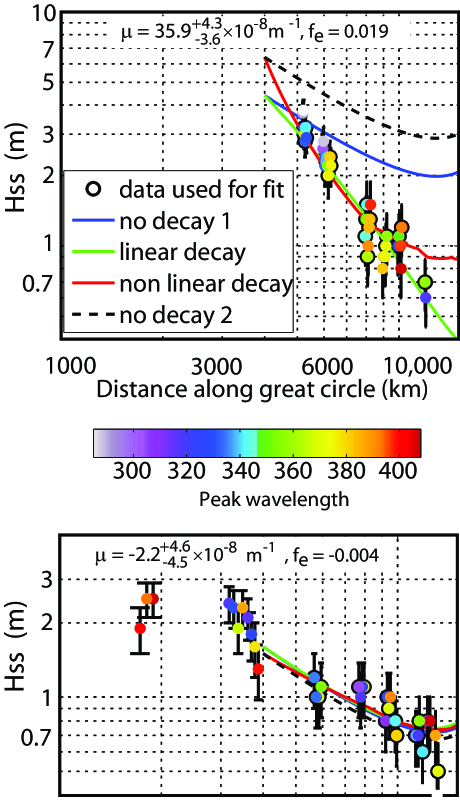
Figure 1: (a) Observed swell wave height as a function of distance, and theoretical decays with fitted constant coefficients using no dissipation, linear ($\mu$ constant) or non-linear ($f_{e}$ constant) dissipation, for the 15 s waves generated by a very strong (top) North Pacific storm on 12 February 2007 (auxiliary table 1: swell number 18) and a weaker (bottom) southern ocean storm on 12 August 2007 (auxiliary table 1: swell number 19). Circled dots are the observations used in the fitting procedure. Error bars show one standard deviation of the expected error on each SAR measurement (Collard et al., 2009).

In each track ensemble, all swells have close initial directions $\theta_{0}$, and the wave field is only a function of $\alpha$. We define the spatial evolution rate

$$\mu=-\frac{\mathrm{d}\left(\alpha\sin\alpha E_{s}\right)/\mathrm{d}\alpha}{R\left(\alpha\sin\alpha E_{s}\right)}.$$ (1)

Positive values of $\mu$ correspond to losses of wave energy (Figure 1.a). Negative, but not significant, values are occasionally found (figure 1.b).

For each track ensemble we take a reference distance $\alpha_{0}=\pi/5$ which corresponds to 4000 km. $\mu$ is estimated by finding the pair $\left(\widehat{E}_{s}(\alpha_{0}),\mu\right)$, that minimizes the mean square difference between observed swell energies $E_{s}(\alpha_{i})$ with $i$ ranging from 1 to $N$, and the theoretical constant linear decay,

$$\widehat{E}_{s}(\alpha_{i})\alpha_{i}\sin\alpha_{i}=\widehat{E}_{s}(\alpha_{0})\alpha_{0}\sin\alpha_{0}{\mathrm{e}}^{-R\mu(\alpha_{i}-\alpha_{0})}.$$ (2)

Because we only have two parameters $\mu$ and $\widehat{E}_{s}(\alpha_{0})$ to adjust, the minimization is performed by a complete search of the parameter space.

Collard et al. (2009) estimated that the SAR-derived swell heights $H_{ss}=4\sqrt{E_{s}}$ are gamma-distributed about a true value $H_{ss}-b_{H}$. The bias is well approximated by

$$b_{H}=0.11+0.1H_{ss}-0.1\max\{0,U_{10SAR}-7\}$$ (3)

with $H_{ss}$ in meters and the wind speed $U_{10}$ in m s^-1. A realistic model of the standard deviation of the measurement error is

$$\sigma_{H}=0.10\mathrm{m}+\min\left\{0.25H_{ss},0.8\mathrm{m}\right\}.$$ (4)

Using this error model, we generated 400 synthetic data sets by perturbing independently each measured swell wave height, in order to obtain a confidence interval for $\mu$. For each swell case, the values of $\mu$ and $H_{ss}(\alpha_{0})$ reported below are the medians of the 400 calculated values.

For all our swell data, $\mu$ ranges from -0.6 to $3.7\times 10^{-7}$ m^-1 (Figure 2.a), comparable to 2.0$\times 10^{-7}$ m^-1 previously reported for large amplitude swells with a 13 s period(Snodgrass et al., 1966). Clarifying earlier observations by Darbyshire (1958) and Snodgrass et al. (1966), our analysis unambiguously proves that swell dissipation increases with the wave steepness. We recall that, in the absence of dissipation, a maximum 20% deviation of $E_{s}$ relative to the asymptote is expected due to the storm shape. This deviation is equal to the one produced by a real 5.0$\times 10^{-8}$ m^-1 dissipation over 4000 km. Thus a comparable error on the estimation of $\mu$ is expected when, as we do here, the storm shape is not taken into account (Collard et al., 2009).

3 Interpretation of swell dissipation

At present there is no consensus on the plausible causes of the loss of swell energy (WISE Group, 2007). Interaction with oceanic turbulence is expected to be relatively small (Ardhuin and Jenkins, 2006). Observed modifications and reversals of the wind stress over swells (Grachev and Fairall, 2001) suggest that some swell momentum is lost to the atmosphere. The wave-induced modulations of air-sea stresses yield a flux of energy from the waves to the wind, due to the correlations of pressure and velocity normal to the sea surface, and the correlations of shear stress and tangential velocity. An upward flux of momentum, readily observed over steep laboratory waves, can thus result in a wave-driven wind (Harris, 1966). If these modulations are linearized (e.g. Kudryavtsev and Makin, 2004), the swell dissipation rate becomes linear in terms of the wave energy, with a proportionality constant that typically depends on the wind, but which does increase with the swell steepness, as we observe here.

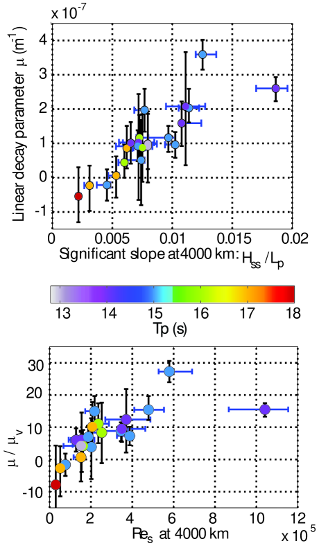
Figure 2: Swell dissipation for 22 events (see auxiliary material for details). (a) Estimated linear attenuation coefficient as a function of the initial significant slope, ratio of the swell significant wave height and peak wavelength, $s=4H_{s}/L$, taken 4000 km from the storm centre, for a variety of peak swell periods (colors). (b) Attenuation coefficient normalized by the viscous attenuation $\mu_{\nu}$ (eq. 5), as a function of the significant swell Reynolds number Re_s determined from significant velocity and displacement amplitudes at 4000 km from the storm.

Our observations show no clear trend with wind magnitude $U_{10}$ and wind-wave angle $\theta_{w}$: the swell age $C/U_{10}$ or $C/(U_{10}\cos\theta_{w})$ averaged over the swell track gives little correlation with $\mu$, even when wheigthed with the swell energy. We thus take a novel approach, and interpret our data by neglecting the effect of the wind, considering only the shear stress modulations induced by swell orbital velocities. Little data are available for air flows over swells, but boundary layers over fixed surfaces are well known, and should have similar properties if their significant orbital amplitudes of velocity and displacement are doubled (Collard et al., 2009). The dissipation then depends on the surface roughness and a significant Reynolds number, $\mathrm{Re}(\varphi)=4u_{\mathrm{orb}}(\varphi)a_{\mathrm{orb}}(\varphi)/\nu$, where $u_{\mathrm{orb}}$ and $a_{\mathrm{orb}}$ are the significant amplitudes of the surface orbital velocities and displacements.

For Re$<10^{5}$, the flow should be laminar (Jensen et al., 1989). The strong shear above the surface makes the air viscosity important, with a dissipation coefficient given by Dore (1978) and Collard et al. (2009)

$$\mu_{\nu}=2\frac{\rho_{a}}{\rho_{w}gC_{g}}\left(\frac{2\pi}{T}\right)^{5/2}\sqrt{2\nu},$$ (5)

where $L$ is the swell wavelength, $L=gT^{2}/(2\pi)$ in deep water with $g$ the acceleration of gravity. At ambient temperature and pressure, the air viscosity is $\nu=1.4\times 10^{-5}$ m²s^-1, and $\mu_{\nu}$ is only a function of $T$. As $T$ increases from 13 to 19 s, $\mu_{\nu}$ decreases from $2.2\times 10^{-8}$ to $5.8\times 10^{-9}$m^-1.

For larger Reynolds numbers the flow becomes turbulent. The energy rate of decay in time can be written as

$$\beta=-\frac{\mathrm{d}E_{s}/\mathrm{d}t}{E_{s}}=C_{g}\mu=\frac{\rho_{a}4\pi^{2}}{\rho_{w}gT^{2}}f_{e}u_{\mathrm{orb}}$$ (6)

where $f_{e}$ is a swell dissipation factor. For a smooth surface, $f_{e}$ is of the order of 0.002 to 0.008 (Jensen et al., 1989), when assumed equal to the friction factor $f_{w}$.

Re is difficult to estimate from the SAR data only, because ENVISAT’s ASAR does not resolve the short windsea waves. However, in deep water we can define the smaller ‘swell Reynolds number’ $\mathrm{Re_{s}}$ from $u_{\mathrm{orb,s}}=2\sqrt{E_{s}}2\pi/T$ and $a_{\mathrm{orb,s}}=2\sqrt{E_{s}}$.

Our estimates of $\mu$ exceed $\mu_{\nu}$ by a factor that ranges from $O(1)$ to 28 (Figure 2.b), quantitatively similar to oscillatory boundary layer over fixed surfaces with no or little roughness. Namely, dissipation rates $\mu$ of the order of the viscous value $\mu_{\nu}$ are found for Re${}_{s}<5\times 10^{4}$ when the the flow may be laminar, and we only find large values of $\mu/\mu_{\nu}$ when Re${}_{s}>5\times 10^{4}$ over a significant portion of the swell track. For reference, a 6.3 m s^-1 wind can generate a fully-developed wind-sea with Re$=2\times 10^{5}$, making the boundary layer turbulent for any swell amplitude. Using the numerical wave model described in Ardhuin et al. (2009), one finds that this value of Re_s translates to Re$\simeq 10^{5}$. That same model also gives values of $u_{\mathrm{orb}}$. Fitting a constant $f_{e}$ for each track ensemble yields $-0.001\leq f_{e}\leq 0.019$, with a median of 0.007, close to what is expected over a smooth surface. This suggests that the roughness of the waves for this oscillatory motion is very small compared to the orbital amplitude.

A parameterization of swell dissipation, taking $f_{e}$ constant in the range 0.0035 to 0.007, generally yields accurate wave heights (not shown). The quality of the end result also depends on the other parameterizations for wind input, whitecapping and wave-wave interactions, and requires a rather lengthy discussion (e.g. Ardhuin et al., 2008, 2009).

Beyond this simple model, we expect that winds should modify the boundary layer over swell, with a significant effect for winds larger than 7 m s^-1 (Collard et al., 2009). Kudryavtsev and Makin (2002) considered the wind stress modulations due to short wave roughness modulated by swells, and found that the preferential breaking of short waves near long wave crests could double the wind-wave coupling coefficient $\mu$ for the long waves. Yet, their linear model cannot explain the nonlinear dissipation observed here, because they only considered lowest order effects. Further investigations should probably consider both wind and finite amplitude swell effects to explain the observed variability of $\mu$.

If this dissipation is due to the proposed air-sea friction mechanism, the associated momentum flux $\rho_{w}gE_{s}/2$ goes to the atmosphere. If, on the contrary, underwater processes dominate, an energy flux $\rho_{w}gC_{g}E_{s}$ may go into ocean turbulence. Accordingly, these fluxes are small. For 3 m high swells, the momentum flux is 8% of the wind stress produced by a 3 m s^-1 wind. This momentum flux thus plays a minor role in observed O(50%) modifications of the wind stress at low wind(Drennan et al., 1999; Grachev and Fairall, 2001). Wind stress modifications are more likely associated with a nonlinear influence of swell on turbulence in the atmospheric boundary layer (Sullivan et al., 2008). This effect may arise as a result of the low-level wave-driven wind jet (Harris, 1966) and its effects on the wind profile around the critical level for the short wave generation (Hristov et al., 2003) . Whatever the actual process, the dissipation coefficient $\mu$ is a key parameter for validating theoretical and numerical models (Kudryavtsev and Makin, 2004; Hanley and Belcher, 2008).

4 Conclusions

Using high quality data from a space-borne synthetic aperture radar, ocean swells were systematically tracked across ocean basins over the years 2003 to 2007. Ten storms provided enough data to allow a total of 22 estimations of the swell energy budget for peak periods of 13 to 18 s. The dissipation of small-amplitude swells is not distinguishable from viscous dissipation, with decay scales larger than 20000 km. On the contrary, steep swells lose a significant fraction of their energy, up to 65% over a distance as short as 2800 km. This non-linear behavior is consistent with a transition from a laminar to a turbulent air-side boundary layer. Many other processes may contribute to the observed dissipation, and a full model of the air-sea interface will be needed for further progress. The present observations and analysis opens the way for a better understanding of air-sea fluxes in low wind conditions, and more accurate hindcasts and forecasts of sea states (see Ardhuin et al., 2008, 2009, and e.g. the SHOM results in Bidlot 2008).

Further investigations are necessary to understand the wind stress modulations and their variations with wind speed, direction, and swell amplitude. Such an effort is essential for the improvement of numerical wave models and their application to remote sensing and the estimation of air-sea fluxes.