A fast approach for overcomplete sparse decomposition based on smoothed $\ell^{0}$ norm

Abstract

In this paper, a fast algorithm for overcomplete sparse decomposition, called SL0, is proposed. The algorithm is essentially a method for obtaining sparse solutions of underdetermined systems of linear equations, and its applications include underdetermined Sparse Component Analysis (SCA), atomic decomposition on overcomplete dictionaries, compressed sensing, and decoding real field codes. Contrary to previous methods, which usually solve this problem by minimizing the $\ell^{1}$ norm using Linear Programming (LP) techniques, our algorithm tries to directly minimize the $\ell^{0}$ norm. It is experimentally shown that the proposed algorithm is about two to three orders of magnitude faster than the state-of-the-art interior-point LP solvers, while providing the same (or better) accuracy.

EDICS Category: MAL-SSEP, SPC-CODC, DSP-FAST

I Introduction

Finding sparse solutions of Under-determined Systems of Linear Equations (USLE) is of significant importance in signal processing and statistics. It is used, for example, in underdetermined Sparse Component Analysis (SCA) and source separation [1, 2, 3, 4], atomic decomposition on overcomplete dictionaries [5, 6], compressed sensing [7, 8], decoding real field codes [9], image deconvolution [10, 11], image denoising [12], electromagnetic imaging and Direction of Arrival (DOA) finding [13]. Despite recent theoretical developments [14, 15, 16, 17], the computational cost of the methods has remained as the main restriction, especially for large systems (large number of unknowns/equations). In this article, a new approach is proposed which provides a considerable reduction in complexity. To introduce the problem in more details, we will use the context of Sparse Component Analysis (SCA). The discussions, however, may be easily followed in other contexts and applications.

SCA can be viewed as a method to achieve separation of sparse sources. Suppose that $m$ source signals are recorded by a set of $n$ sensors, each of which records a combination of all sources. In linear instantaneous (noiseless) model, it is assumed that ${\bf x}(t)={\bf A}{\bf s}(t)$ in which ${\bf x}(t)$ and ${\bf s}(t)$ are the $n\times 1$ and $m\times 1$ vectors of source and recorded signals, respectively, and ${\bf A}$ is the $n\times m$ (unknown) mixing matrix. The goal of Blind Source Separation (BSS) [18, 19] is then to find ${\bf s}(t)$ only by observing ${\bf x}(t)$. The general BSS problem is impossible for the case $m>n$. However, if the sources are sparse (i.e., not a totally blind situation), then the problem can be solved in two steps [1, 2]: first estimating the mixing matrix, and then estimating the sources assuming ${\bf A}$ being known. For sparse sources, the first step – which can become very tricky for large $m$ – may be accomplished by means of clustering [1, 2, 20, 21]. The second step requires that for each sample ($t_{0}$) the sparse solution of the USLE ${\bf x}(t_{0})={\bf A}{\bf s}(t_{0})$ be found [1, 2, 22, 23]. Note also that the sparsity of the sources is not necessarily in the time domain: if $T\{.\}$ is a linear ‘sparsifying’ transformation, then $T\{{\bf x}\}={\bf A}\,T\{{\bf s}\}$. Due to linearity of $T$, both the linearity of the mixing and the statistical independence properties of sources are preserved in the transformed domain. Hence, SCA may be applied in the transformed domain.

In the atomic decomposition viewpoint [5], the signal vector ${\bf x}=[x(1),\dots,x(n)]^{T}$ is composed of the samples of a ‘single’ signal $x(t)$, and the objective is to represent it as a linear combination of $m$, $n\times 1$ signal vectors $\{{\bf a}_{i}\}_{i=1}^{m}$. After [24], the vectors ${\bf a}_{i}$, $1\leq i\leq m$ are called atoms and they collectively form a dictionary over which the signal is to be decomposed. We may write ${\bf x}=\sum_{i=1}^{m}s_{i}{\bf a}_{i}={\bf A}{\bf s}$, where ${\bf A}\triangleq[{\bf a}_{1},\dots,{\bf a}_{m}]$ is the $n\times m$ dictionary (matrix) and ${\bf s}\triangleq(s_{1},\dots,s_{m})^{T}$ is the $m\times 1$ vector of coefficients. A dictionary with $m>n$ is called overcomplete. Although, $m=n$ (e.g. Discrete Fourier Transform) is sufficient to obtain such a decomposition, using overcomplete dictionaries has a lot of advantages in many diverse applications (refer for example to [6] and the references in it). In all these applications, we would like to use as small as possible number of atoms to represent the signal. Again, we have the problem of finding sparse solutions of the USLE ${\bf A}{\bf s}={\bf x}$.

To obtain the sparsest solution of ${\bf A}{\bf s}={\bf x}$, we may search for a solution with minimal $\ell^{0}$ norm, i.e., minimum number of nonzero components. It is usually stated in the literature [6, 9, 4] that searching the minimum $\ell^{0}$ norm is an intractable problem as the dimension increases (because it requires a combinatorial search), and it is too sensitive to noise (because any small amount of noise completely changes the $\ell^{0}$ norm of a vector). Consequently, researchers consider other approaches. One of the most successful approaches is Basis Pursuit (BP) [5, 15, 4, 25] which finds the minimum $\ell^{1}$ norm (that is, the solution of ${\bf A}{\bf s}={\bf x}$ for which $\sum_{i}{|s_{i}|}$ is minimized). Such a solution can be easily found by Linear Programming (LP) methods. The idea of Basis Pursuit is based on the observation that for large systems of equations, the minimum $\ell^{1}$ norm solution is also the minimum $\ell^{0}$ norm solution [14, 15, 5]. By using fast LP algorithms, specifically interior-point LP solvers, large-scale problems with thousands of sources and mixtures become tractable. However, it is still very slow, and in the recent years several authors have proposed improvements for BP, to speed up the algorithm and to handle the noisy case [16, 6, 10, 11]. Another family of algorithms is Iterative Re-weighted Least Squares (IRLS), with FOCUSS [13] as an important member. These are faster than BP, but their estimation quality is worse, especially if the number of non-zero elements of the sparsest solution is not very small. Another approach is Matching Pursuit (MP) [24, 26, 1] which is very fast, but is a greedy algorithm and does not provide good estimation of the sources. The approach presented in [27] is also very fast, but adjusting its parameters is not easy.

Contrary to previous approaches, the method we present in this paper is based on direct minimization of the $\ell^{0}$ norm. We will see that our method performs typically two to three orders of magnitude faster than BP (based on interior-point LP solvers), while resulting in the same or better accuracy. We have already briefly reported the basics of this approach in [28] and its complex version in [29]. However, in this paper, we are going to present a highly more complete description of this approach and consider, mathematically and/or experimentally, its convergence properties and the effects of its parameters.

The paper is organized as follows. The next section introduces the basic principles of our approach. The final algorithm is then stated in Section III. In Section IV, convergence properties of the algorithm is discussed. Finally, Section V provides some experimental results of our algorithm and its comparison with BP.

II Basic Principles Of Our Approach

II-A The Main Idea

The problems of using $\ell^{0}$ norm (that is, the need for a combinatorial search for its minimization, and its too high sensibility to noise) are both due to the fact that the $\ell^{0}$ norm of a vector is a discontinuous function of that vector. Our idea is then to approximate this discontinuous function by a suitable continuous one, and minimize it by means of a minimization algorithm for continuous functions (e.g. steepest descent method). The continuous function which approximates $\|{\bf s}\|_{0}$, the $\ell^{0}$ norm of ${\bf s}$, should have a parameter (say $\sigma$) which determines the quality of the approximation.

For example, consider the (one-variable) family of functions:

$$f_{\sigma}(s)\triangleq\exp{(-s^{2}/2\sigma^{2})},$$ (1)

and note that:

$$\lim_{\sigma\to 0}f_{\sigma}(s)=\left\{\begin{array}[]{ll}1&;\mbox{if $s=0$}\\ 0&;\mbox{if $s\neq 0$}\end{array}\right.,$$ (2)

or approximately:

$$f_{\sigma}(s)\approx\left\{\begin{array}[]{ll}1&;\mbox{if $|s|\ll\sigma$}\\ 0&;\mbox{if $|s|\gg\sigma$}\end{array}\right..$$ (3)

Then, by defining:

$$F_{\sigma}({\bf s})=\sum_{i=1}^{m}f_{\sigma}(s_{i}),$$ (4)

it is clear from (2) and (3) that $\|{\bf s}\|_{0}\approx m-F_{\sigma}({\bf s})$ for small values of $\sigma$, and the approximation tends to equality when $\sigma\to 0$. Consequently, we can find the minimum $\ell^{0}$-norm solution by maximizing $F_{\sigma}({\bf s})$ (subject to ${\bf A}{\bf s}={\bf x}$) for a very small value of $\sigma$. Note that the value of $\sigma$ determines how smooth the function $F_{\sigma}$ is: the larger value of $\sigma$, the smoother $F_{\sigma}$ (but worse approximation to $\ell^{0}$-norm); and the smaller value of $\sigma$, the closer behavior of $F_{\sigma}$ to $\ell^{0}$-norm.

Note that for small values of $\sigma$, $F_{\sigma}$ is highly non-smooth, and contains a lot of local maxima, and hence its maximization is not easy. On the other hand, for larger values of $\sigma$, $F_{\sigma}$ is smoother and contains less local maxima, and its maximization is easier (we will see in the next subsection that there is no local maxima for large enough $\sigma$’s). Consequently, our idea is to use a ‘decreasing’ sequence for $\sigma$: for maximizing $F_{\sigma}$ for each value of $\sigma$ (using e.g. gradient algorithms), the initial value of the maximization algorithm is the maximizer of $F_{\sigma}$ for the previous (larger) value of $\sigma$. If we gradually decrease the value of $\sigma$, for each value of $\sigma$ the maximization algorithm starts with an initial solution near to the actual maximizer of $F_{\sigma}$ (this is because $\sigma$ and hence $F_{\sigma}$ have only slightly changed and consequently the maximum of the new $F_{\sigma}$ is eventually near to the maximum of the previous $F_{\sigma}$), and hence we eventually escape from getting trapped into local maxima and reach to the actual maximum for small values of $\sigma$, which gives the minimum $\ell^{0}$-norm solution.

Note that the basic idea holds not only for Gaussian family of functions $f_{\sigma}$ given in (1), but also for any family of functions $f_{\sigma}$ which approximates the Kronecker delta function, i.e., satisfies (2) and (3). For example, it also holds for the family of ‘triangular’ functions:

$$f_{\sigma}(s)=\left\{\begin{array}[]{ll}1&;\mbox{if $|s|\geq\sigma$}\\ (\sigma+s)/\sigma&;\mbox{if $-\sigma\leq s\leq 0$}\\ (\sigma-s)/\sigma&;\mbox{if $0\leq s\leq\sigma$}\end{array}\right.,$$ (5)

and for the family of ‘truncated hyperbolic’ functions:

$$f_{\sigma}(s)=\left\{\begin{array}[]{ll}1&;\mbox{if $|s|\geq\sigma$}\\ 1-(s/\sigma)^{2}&;\mbox{if $|s|\leq\sigma$}\\ \end{array}\right.,$$ (6)

and also for the family of functions:

$$f_{\sigma}(s)=\sigma^{2}/(s^{2}+\sigma^{2}).$$ (7)

II-B Initialization

Up to now, the behavior of the function $f_{\sigma}$ was discussed for small values of $\sigma$. It is also interesting to consider the behavior for very large values of $\sigma$.

More specifically, it can be shown that “for sufficiently large values of $\sigma$, the maximizer of $F_{\sigma}({\bf s})$ subject to ${\bf A}{\bf s}={\bf x}$ is the minimum $\ell^{2}$-norm solution of ${\bf A}{\bf s}={\bf x}$, i.e., the solution given by the pseudo-inverse of ${\bf A}$”. Here, we give only a justification to this property for the case of Gaussian family of functions introduced in (1) by using Lagrange multipliers, and we leave the formal proof to Section IV-B.

Using the method of Lagrange multipliers, for maximizing $F_{\sigma}({\bf s})=\sum_{i=1}^{m}f_{\sigma}(s_{i})=\sum_{i=1}^{m}\exp{(-s_{i}^{2}/2\sigma^{2})}$ subject to ${\bf A}{\bf s}={\bf x}$, we set the derivative of the Lagrangian ${\cal L}({\bf s},\boldsymbol{\lambda})=F_{\sigma}({\bf s})-\boldsymbol{\lambda}^{T}({\bf A}{\bf s}-{\bf x})$ with respect to ${\bf s}$ and $\boldsymbol{\lambda}$ equal to zero, which gives the following Karush-Kuhn-Tucker (KKT) system of $m+n$ nonlinear equations of $m+n$ unknowns ($m$ components of ${\bf s}$, and $n$ components of $\boldsymbol{\lambda}$):

$$\left\{\begin{array}[]{ll}[s_{1}e^{-s_{1}^{2}/2\sigma^{2}},\dots,s_{m}e^{-s_{m}^{2}/2\sigma^{2}}]^{T}-{\bf A}^{T}\boldsymbol{\lambda}_{1}={\bf 0}\\ {\bf A}{\bf s}-{\bf x}={\bf 0}\end{array}\right.$$ (8)

where $\boldsymbol{\lambda}_{1}\triangleq-\sigma^{2}\boldsymbol{\lambda}$.

On the other hand, the minimum $\ell^{2}$ norm solution of ${\bf A}{\bf s}={\bf x}$ may be found by minimizing $\frac{1}{2}{\bf s}^{T}{\bf s}$ subject to ${\bf A}{\bf s}={\bf x}$. Using Lagrange multipliers, this minimization results in the system of equations:

$$\left\{\begin{array}[]{ll}[s_{1},\dots,s_{m}]^{T}-{\bf A}^{T}\boldsymbol{\lambda}={\bf 0}\\ {\bf A}{\bf s}-{\bf x}={\bf 0}\end{array}\right.$$ (9)

Comparing systems (8) and (9), we see that for $\sigma\to\infty$ (or where $\sigma\gg\max\{s_{1},\dots,s_{m}\}$), these two systems of equations are identical, and hence the maximizer of $F_{\sigma}({\bf s})$ is the minimum $\ell^{2}$-norm solution of ${\bf A}{\bf s}={\bf x}$.

III The Final Algorithm

The final algorithm, which we call SL0 (Smoothed $\ell^{0}$), is obtained by applying the main idea of the previous section on the Gaussian family (1), and is given in Fig. 1.

    • Initialization: 1. Let ${\bf\hat{s}}_{0}$ be equal to the minimum $\ell^{2}$ norm solution of ${\bf A}{\bf s}={\bf x}$, obtained by pseudo-inverse of ${\bf A}$. 2. Choose a suitable decreasing sequence for $\sigma$, $[\sigma_{1}\ldots\sigma_{J}]$ (see Remarks 5 and 6 of the text). • For $j=1,\dots,J$:
  1. Let $\sigma=\sigma_{i}$. 2. Maximize (approximately) the function $F_{\sigma}$ on the feasible set ${\mathcal{S}}=\{{\bf s}\,|\,{\bf A}{\bf s}={\bf x}\}$ using $L$ iterations of the steepest ascent algorithm (followed by projection onto the feasible set): – Initialization: ${\bf s}={\bf\hat{s}}_{j-1}$. – For $\ell=1\dots L$ (loop $L$ times):
  (a) Let $\boldsymbol{\delta}\triangleq[s_{1}\exp{(-s_{1}^{2}/2\sigma^{2})},\dots,s_{n}\exp{(-s_{n}^{2}/2\sigma^{2})}]^{T}$. (b) Let ${\bf s}\leftarrow{\bf s}-\mu\boldsymbol{\delta}$ (where $\mu$ is a small positive constant). (c) Project ${\bf s}$ back onto the feasible set ${\mathcal{S}}$: $${\bf s}\leftarrow{\bf s}-{\bf A}^{T}({\bf A}{\bf A}^{T})^{-1}({\bf A}{\bf s}-{\bf x}).$$
  3. Set ${\bf\hat{s}}_{j}={\bf s}$.
  • Final answer is ${\bf\hat{s}}={\bf\hat{s}}_{J}$.    

Figure 1: The final SL0 algorithm.

Remark 1.   The internal loop (steepest ascent for a fixed $\sigma$) is repeated a fixed and small number of times ($L$). In other words, for increasing the speed, we do not wait for the (internal loop of the) steepest ascent algorithm to converge. This may be justified by the gradual decrease in the value of $\sigma$, and the fact that for each value of $\sigma$, we do not need the exact maximizer of $F_{\sigma}$. We just need to enter the region near the (global) maximizer of $F_{\sigma}$ for escaping from its local maximizers. See also Remarks 3 to 5 of Section IV-A.

Remark 2.   Steepest ascent consists of iterations of the form ${\bf s}\leftarrow{\bf s}+\mu_{j}\nabla F_{\sigma}({\bf s})$. Here, the step-size parameters $\mu_{j}$ should be decreasing, i.e., for smaller values of $\sigma$, smaller values of $\mu_{j}$ should be applied. This is because for smaller values of $\sigma$, the function $F_{\sigma}$ is more ‘fluctuating’, and hence smaller step-sizes should be used for its maximization. In fact, we may think about changing the value of $\sigma$ in (1) and (4) as looking at the same curve (or surface) at different ‘scales’, where the scale is proportional to $\sigma$. For having equal (i.e., proportional) steps of the steepest ascent algorithm in these different scales, it is not difficult to show that $\mu_{j}$ should be proportional to $\sigma^{2}$. Note that in Fig. 1, instead of $\mu_{j}$, only a constant $\mu$ is appeared. The reason is that by letting $\mu_{j}=\mu\sigma^{2}$ for some constant $\mu$, we have ${\bf s}\leftarrow{\bf s}+(\mu\sigma^{2})\nabla F_{\sigma}={\bf s}-\mu\boldsymbol{\delta}$, where $\boldsymbol{\delta}\triangleq-\sigma^{2}\,\nabla F_{\sigma}=[s_{1}\exp{(-s_{1}^{2}/2\sigma^{2})},\dots,s_{n}\exp{(-s_{n}^{2}/2\sigma^{2})}]^{T}$.

Remark 3.   According to the algorithm, each iteration consists of an ascent step $s_{i}\leftarrow s_{i}-\mu s_{i}\exp(-s_{i}^{2}/2\sigma^{2}),\,1\leq i\leq m$, followed by a projection step. If for some values of $i$ we have $|s_{i}|\gg\sigma$, then the algorithm does not change the value of $s_{i}$ in that ascent step; however it might be changed in the projection step. If we are looking for a suitable large $\mu$ (to reduce the required number of iterations), a suitable choice is to make the algorithm to force all those values of $s_{i}$ satisfying $|s_{i}|\lesssim\sigma$ toward zero. For this aim, we should have $\mu\exp(-s_{i}^{2}/2\sigma^{2})\approx 1$, and because $\exp(-s_{i}^{2}/2\sigma^{2})\lesssim 1$ for $|s_{i}|\lesssim\sigma$, the choice $\mu\gtrsim 1$ seems reasonable.

Remark 4.   The algorithm may work by initializing ${\bf\hat{s}}_{0}$ (the initial estimation of the sparse solution) to an arbitrary solution of ${\bf A}{\bf s}={\bf x}$. However, the discussion of Section II-B shows that the best initial value of ${\bf\hat{s}}_{0}$ is the minimum $\ell^{2}$ norm solution of ${\bf A}{\bf s}={\bf x}$, which corresponds to $\sigma\to\infty$. In another point of view, one may think about the minimum $\ell^{2}$ norm solution as a rough estimate of the sparse solution, which will be modified in the future iterations of the algorithm. In fact, calculating minimum $\ell^{2}$ norm is one of the earliest approaches used for estimating the sparsest solution and is called the Method Of Frames (MOF) [5].

Remark 5.   Having initiated the algorithm with the minimum $\ell^{2}$ norm solution (which corresponds to $\sigma=\infty$), the next value for $\sigma$ (i.e., $\sigma_{1}$) may be chosen about two to four times of the maximum absolute value of the obtained sources ($\max_{i}|s_{i}|$). To see the reason, if we take for example $\sigma>4\max_{i}|s_{i}|$, then $\exp(-s_{i}^{2}/2\sigma^{2})>0.96\approx 1$ for all $1\leq i\leq m$, and comparison with (3) shows that this value of $\sigma$ acts virtually like infinity for all the values of $s_{i}$, $1\leq i\leq m$ (the next remark, too, provides another reason through another viewpoint to the algorithm).

For the next values of $\sigma$, we have used $\sigma_{j}=c\,\sigma_{j-1}$, $j\geq 2$, where $c$ is usually chosen between 0.5 and 1. Its effect is experimentally studied in Section V).

Remark 6.   Equation (4) seems to simply count the “inactive” elements of ${\bf s}$. However, instead of hard-thresholding “$\mbox{inactive}\equiv|s_{i}|<\sigma\,;\mbox{ active}\equiv|s_{i}|>\sigma$”, criterion (4) uses a soft-thresholding, for which $\sigma$ is the rough threshold.

Remark 7.   In applications where the zeros in the sparsest ${\bf s}$ are exactly zero, $\sigma$ can be decreased arbitrarily. In fact, in this case, its minimum value is determined by the desired accuracy, as will be discussed in Theorem 1. For applications in which inactive elements of ${\bf s}$ are small but not exactly zero (say that the ‘source’ vector is noisy), the smallest $\sigma$ should be about one to two times of (a rough estimation of) the standard deviation of this noise. This is because, while $\sigma$ is in this range, (3) shows that the cost function treats small (noisy) samples as zeros (i.e., for which $f_{\sigma}(s_{i})\approx 1$). However, below this range, the algorithm tries to ‘learn’ these noisy values, and moves away from the true answer (according to the previous remark, the soft threshold should be such that all these noisy samples be considered inactive). Restricting $\sigma_{i}$ to be above the standard deviation of the noise, provides the robustness of this approach to noisy sources (or mixtures), which was one of the difficulties in using the exact $\ell^{0}$ norm.

IV Theoretical Analysis of the Algorithm

IV-A Convergence Analysis

In this section, we try to answer two questions for the noiseless case (the noisy case will be considered in Section IV-C): a) Does the basic idea of Section II results in convergence to the actual minimizer of the $\ell^{0}$ norm (assumed to be unique by [13, 15])? and b) If yes, how much should we decrease $\sigma$ to achieve a desired accuracy?

Note that the algorithm of Fig. 1 has two loops: the external loop which corresponds to the basic ideas of Section II for finding the sparsest solution, and the internal loop which is a simple steepest ascent algorithm for maximizing $F_{\sigma}({\bf s})$ for a fixed $\sigma$. In the analysis of this section, it is assumed that the maximization of $F_{\sigma}({\bf s})$ has been exactly done for a fixed $\sigma$ (the maximization algorithm has not got trapped into local maxima). Note that we had proposed the gradual decrease in $\sigma$ to escape from getting trapped into local maxima when maximizing $F_{\sigma}$ for a fixed $\sigma$. A theoretical study to find the series $\sigma_{j}$, $j=1,\ldots J$, which guaranties the convergence is very tricky (if possible) and is not considered in this paper. However, it will be experimentally addressed in the next section.

Assuming the maximization of $F_{\sigma}$ for fixed $\sigma$’s is perfectly done, we show here that the estimation given by the algorithm converges to the unique minimizer of the $\ell^{0}$ norm. In other words, we prove that the sequence of ‘global’ maximizers of $F_{\sigma}$’s will converge to the sparsest solution (which is the basic idea of Section II), and try to answer both above questions.

Before stating the convergence theorem (Theorem 1), we state three lemmas. Recall that $\mathrm{null}({\bf A})=\{{\bf s}|{\bf A}{\bf s}={\bf 0}\}$.

Lemma 1

Assume that the matrix ${\bf A}=[{\bf a}_{1},{\bf a}_{2},\cdots,{\bf a}_{m}]\in\mathbb{R}^{n\times m}$ (where ${\bf a}_{i}$ represents the $i$-th column) has the property that all of its $n\times n$ sub-matrices are invertible, which is called the Unique Representation Property (URP) in [13]. If $m-n$ elements of ${\bf s}\in\mathrm{null}({\bf A})$ converge to zero, then all of its elements (and hence ${\bf s}$) will converge to zero, too.

Proof:

Without loss of generality, assume that all the columns of ${\bf A}$ are normalized, i.e. $\|{\bf a}_{i}\|=1$, $1\leq i\leq m$ (throughout the paper, $\|\cdot\|$ stands for the $\ell^{2}$ or Euclidean or Frobenius norm of a vector or matrix). Then, we have to show:

$$\begin{split}&\forall\beta>0,\quad\exists\alpha>0,\quad\mbox{such that }\forall{\bf s}\in\mathrm{null}({\bf A}):\\ &\mbox{$m-n$ elements of ${\bf s}$ have absolute values}\\ &\qquad\qquad\qquad\mbox{less than $\alpha$}\Rightarrow\|{\bf s}\|\leq\beta\end{split}$$ (10)

Let ${\bf s}=(s_{1},s_{2},\cdots,s_{m})^{T}$ be in $\mathrm{null}({\bf A})$ and assume that the absolute values of at least $m-n$ elements of it are smaller than $\alpha$. Let $I_{\alpha}$ be the set of all indices $i$, for which $|s_{i}|>\alpha$. Consequently, $|I_{\alpha}|\leq n$, where $|X|$ represents the cardinality (i.e., number of elements) of a set $X$. Then we write:

$$\begin{split}\sum_{i=1}^{m}{s_{i}{\bf a}_{i}}={\bf 0}\Rightarrow\sum_{i\in I_{\alpha}}{s_{i}{\bf a}_{i}}+\sum_{i\notin I_{\alpha}}{s_{i}{\bf a}_{i}}={\bf 0}\Rightarrow\\ \|\sum_{i\in I_{\alpha}}{s_{i}{\bf a}_{i}}\|=\|\sum_{i\notin I_{\alpha}}{s_{i}{\bf a}_{i}}\|\leq\sum_{i\notin I_{\alpha}}{\|s_{i}{\bf a}_{i}\|}=\\ \sum_{i\notin I_{\alpha}}{\underbrace{|s_{i}|}_{\leq\alpha}\underbrace{\|{\bf a}_{i}\|}_{1}}\leq\sum_{i\notin I_{\alpha}}{\alpha}=(m-|I_{\alpha}|)\alpha\leq m\alpha\end{split}$$ (11)

Let ${\bf\hat{{\bf A}}}$ be the sub-matrix of ${\bf A}$ containing only those columns of ${\bf A}$ that are indexed by the elements of $I_{\alpha}$. Thus ${\bf\hat{{\bf A}}}$ has at most $n$ columns, and the columns of ${\bf\hat{{\bf A}}}$ are linearly independent, because of the URP of ${\bf A}$. Therefore, there exists a left inverse ${\bf\hat{{\bf A}}}^{-1}$ for ${\bf\hat{{\bf A}}}$. Let $\bar{{\bf s}}$ and ${\bf\tilde{s}}$ denote those sub-vectors of ${\bf s}$ which are, and which are not indexed by $I_{\alpha}$, respectively. Then:

$$\begin{split}\sum_{i\in I_{\alpha}}{s_{i}{\bf a}_{i}}=&{\bf\hat{{\bf A}}}\bar{{\bf s}}\Rightarrow\|\bar{{\bf s}}\|=\|({\bf\hat{{\bf A}}}^{-1})(\sum_{i\in I_{\alpha}}{s_{i}{\bf a}_{i}})\|\\ &\leq\|{\bf\hat{{\bf A}}}^{-1}\|\cdot\|\sum_{i\in I_{\alpha}}{s_{i}{\bf a}_{i}}\|\leq\|{\bf\hat{{\bf A}}}^{-1}\|(m\alpha)\end{split}$$ (12)

$$\begin{split}&\left.\begin{array}[]{l}\|{\bf\tilde{s}}\|\leq\sum_{i\notin I_{\alpha}}{|s_{i}|}\leq(m-|I_{\alpha}|)\alpha\leq m\alpha\\ \|\bar{{\bf s}}\|\leq\|{\bf\hat{{\bf A}}}^{-1}\|m\alpha\end{array}\right\}\Rightarrow\\ &\qquad\qquad\qquad\|{\bf s}\|\leq\|{\bf\tilde{s}}\|+\|\bar{{\bf s}}\|\leq(\|{\bf\hat{{\bf A}}}^{-1}\|+1)m\alpha\end{split}$$ (13)

Now, let $\mathcal{M}$ be the set of all submatrices ${\bf\hat{{\bf A}}}$ of ${\bf A}$, consisting of at most $n$ columns of ${\bf A}$. Then $\mathcal{M}$ is clearly a finite set (in fact $|\mathcal{M}|<2^{m}$). Let

$$M=\max\{\|{\bf\hat{{\bf A}}}^{-1}\|_{\,}\,\,\,|\,{\bf\hat{{\bf A}}}\in\mathcal{M}\},$$ (14)

then

$$\|{\bf s}\|\leq(\|{\bf\hat{{\bf A}}}^{-1}\|+1)m\alpha\leq(M+1)m\alpha.$$ (15)

$M$ is a constant and its value depends only on the matrix ${\bf A}$. Therefore, for each $\beta$ it suffices to choose $\alpha=\beta/m(M+1)$. ∎

The above proof (calculations (11) to (15)) results also in the following corollary:

Corollary 1

If ${\bf A}\in\mathbb{R}^{n\times m}$ satisfies URP, and ${\bf s}\in\mathrm{null}({\bf A})$ has at most $n$ elements with absolute values greater than $\alpha$, then $\|{\bf s}\|<(M+1)m\alpha$, where $M$ is as defined in (14).

Lemma 2

Let a function $f_{\sigma}(s)$ have the properties $f_{\sigma}(0)=1$ and $\forall s,0\leq f_{\sigma}(s)\leq 1$, and let $F_{\sigma}({\bf s})$ be defined as in (4). Assume ${\bf A}$ satisfies the URP, and let ${\mathcal{S}}\triangleq\{{\bf s}\,|\,{\bf A}{\bf s}={\bf x}\}$. Assume that there exists a (sparse) solution ${\bf s}^{0}\in{\mathcal{S}}$ for which $\|{\bf s}^{0}\|_{0}=k\leq n/2$ (such a sparse solution is unique [13, 15]). Then, if for a solution ${\bf\hat{s}}=(\hat{s}_{1},\dots,\hat{s}_{m})^{T}\in{\mathcal{S}}$:

$$F_{\sigma}({\bf\hat{s}})\geq m-(n-k),$$ (16)

and if $\alpha>0$ is chosen such that the $\hat{s}_{i}$’s with absolute values greater than $\alpha$ satisfy $f_{\sigma}(\hat{s}_{i})\leq\frac{1}{m}$, then:

$$\|{\bf\hat{s}}-{\bf s}^{0}\|<(M+1)m\alpha,$$ (17)

where $M$ is as defined in (14).

Proof:

Let $I_{\alpha}$ be the set of all indices $i$ for which $|\hat{s}_{i}|>\alpha$, and denote its number of elements by $|I_{\alpha}|$. Then:

$$\begin{split}F_{\sigma}({\bf\hat{s}})&=\sum_{i=1}^{m}f_{\sigma}(\hat{s}_{i})\\ &=\underbrace{\sum_{i\notin I_{\alpha}}\underbrace{f_{\sigma}(\hat{s}_{i})}_{\leq 1}}_{\leq m-|I_{\alpha}|}+\underbrace{\sum_{i\in I_{\sigma}}\underbrace{f_{\sigma}(\hat{s}_{i})}_{<\frac{1}{m}}}_{<m\cdot\frac{1}{m}=1}<m-|I_{\alpha}|+1.\end{split}$$

Combining this result with (16), we obtain:

$$\begin{split}m-(n-k)\leq F_{\sigma}({\bf\hat{s}})<m-|I_{\alpha}|+1\\ \Rightarrow|I_{\alpha}|<n-k+1\Rightarrow|I_{\alpha}|\leq n-k.\end{split}$$

Consequently, at most $n-k$ elements of ${\bf\hat{s}}$ have absolute values greater than $\alpha$. Since ${\bf s}^{0}$ has exactly $k$ non-zero elements, we conclude that ${\bf\hat{s}}-{\bf s}^{0}$ has at most $(n-k)+k=n$ elements with absolute values greater than $\alpha$. Moreover, $({\bf\hat{s}}-{\bf s}^{0})\in\mathrm{null}({\bf A})$ (because ${\bf A}({\bf\hat{s}}-{\bf s}^{0})={\bf x}-{\bf x}={\bf 0}$), and hence Corollary 1 implies (17). ∎

Corollary 2

For the Gaussian family (1), if (16) holds for a solution ${\bf\hat{s}}$, then:

$$\|{\bf\hat{s}}-{\bf s}^{0}\|<(M+1)m\sigma\sqrt{2\ln m}\,.$$ (18)

Proof:

For Gaussian family (1), the $\alpha$ of the above lemma can be chosen as $\alpha=\sigma\sqrt{2\ln m}$, because for $|\hat{s}_{i}|>\sigma\sqrt{2\ln m}$:

$$f_{\sigma}({\hat{s}_{i}})=\exp\left\{-\frac{\hat{s}_{i}^{2}}{2\sigma^{2}}\right\}<\exp\left\{-\frac{\sigma^{2}\cdot 2\ln m}{2\sigma^{2}}\right\}=\frac{1}{m}.$$

Moreover, this family satisfies the other conditions of the lemma. ∎

Lemma 3

Let $f_{\sigma}$, $F_{\sigma}$, ${\mathcal{S}}$ and ${\bf s}^{0}$ be as in Lemma 2, and let ${\bf s}^{\sigma}$ be the maximizer of $F_{\sigma}({\bf s})$ on ${\mathcal{S}}$. Then ${\bf s}^{\sigma}$ satisfies (16).

Proof:

We write:

$$F_{\sigma}({\bf s}^{\sigma}) \geq F_{\sigma}({\bf s}^{0}) {\bf s}^{\sigma}$$ (because is the maximizer)

$$\geq m-k$$ (see below) (19)

$$\geq m-(n-k) k\leq\frac{n}{2}$$ (because ).

The second inequality was written because ${\bf s}^{0}$ has $m-k$ zeros, and hence in the summation (4) there are $m-k$ ones, and the other terms are non-negative. ∎

Note that Lemma 3 and Corollary 2 prove together that for the Gaussian family (1), $\mathop{\rm argmax}_{{\bf A}{\bf s}={\bf x}}F_{\sigma}({\bf s})\to{\bf s}^{0}$ as $\sigma\to 0$. This result can, however, be stated for a larger class of functions $f_{\sigma}$, as done in the following Theorem.

Theorem 1

Consider a family of univariate functions $f_{\sigma}$, indexed by $\sigma$, $\sigma\in\mathbb{R}^{+}$, satisfying the set of conditions:

1. $\lim_{\sigma\to 0}f_{\sigma}(s)=0\qquad\textrm{; for all }s\neq 0$

2. ${f_{\sigma}(0)}=1\qquad\textrm{; for all }\sigma\in\mathbb{R}^{+}$

3. $0\leq f_{\sigma}(s)\leq 1\qquad\textrm{; for all }\sigma\in\mathbb{R}^{+},s\in\mathbb{R}$

4. For each positive values of $\nu$ and $\alpha$, there exists $\sigma_{0}\in\mathbb{R}^{+}$ that satisfies:

   $$|s|>\alpha\Rightarrow f_{\sigma}(s)<\nu\quad\textrm{; for all }\sigma<\sigma_{0}.$$ (20)

Assume ${\bf A}$ satisfies the URP, and let ${\mathcal{S}}$, $F_{\sigma}$ and ${\bf s}^{0}$ be as defined in Lemma 2, and ${\bf s}^{\sigma}=(s^{\sigma}_{1},\dots,s^{\sigma}_{m})^{T}$ be the maximizer of $F_{\sigma}({\bf s})$ on ${\mathcal{S}}$. Then:

$$\lim_{\sigma\to 0}{{\bf s}^{\sigma}}={\bf s}^{0}.$$ (21)

Proof:

To prove (21), we have to show that:

$$\forall\beta>0\quad\exists\sigma_{0}>0,\quad\forall\sigma<\sigma_{0}\quad\|{\bf s}^{\sigma}-{\bf s}^{0}\|<\beta.$$ (22)

For each $\beta$, let $\alpha=\beta/m(M+1)$, where $M$ is as defined in (14). Then for this $\alpha$ and $\nu=\frac{1}{m}$, condition 4 of the theorem gives a $\sigma_{0}$ for which (20) holds. We show that this is the $\sigma_{0}$ we were seeking for in (22). Note that $\forall\sigma<\sigma_{0}$, (20) states that for $s^{\sigma}_{i}$ ’s with absolute values greater than $\alpha$ we have $f_{\sigma}(s^{\sigma}_{i})<\frac{1}{m}$. Moreover, Lemma 3 states that ${\bf s}^{\sigma}$ satisfies (16). Consequently, all the conditions of Lemma 2 have been satisfied, and hence it implies that $\|{\bf s}^{\sigma}-{\bf s}^{0}\|<(M+1)m\alpha=\beta$. ∎

Remark 1.   The Gaussian family (1) satisfies conditions 1 through 4 of Theorem 1. In fact, conditions 1, 2 and 3 are obvious. To see condition 4, it is sufficient to choose $\sigma_{0}^{2}=-\alpha^{2}/(2\ln{\nu})$ if $\nu<1$, or to choose any arbitrary $\sigma_{0}^{2}\in\mathbb{R}^{+}$ if $\nu\geq 1$. Families of functions defined by (5), (6) and (7) also satisfy the conditions of this theorem.

Remark 2.   Using Corollary 2, where using Gaussian family (1), to ensure an arbitrary accuracy $\beta$ in estimation of the sparse solution ${\bf s}^{0}$, it suffices to choose:

$$\sigma<\frac{\beta}{m\sqrt{2\ln{m}}(M+1)},$$

and do the optimization of $F_{\sigma}$ subject to ${\bf A}{\bf s}={\bf x}$.

Remark 3.   Consider the set of solutions ${\bf\hat{s}}^{\sigma}$ in ${\mathcal{S}}$, which might not be the absolute maxima of functions $F_{\sigma}$ on ${\mathcal{S}}$, but satisfy the condition

$$F_{\sigma}({\bf\hat{s}}^{\sigma})\geq m-(n-k).$$ (23)

By following a similar approach to the proof of Theorem 1, it can be proved that $\lim_{\sigma\to 0}{\bf\hat{s}}^{\sigma}={\bf s}^{0}$. In other words, for the steepest ascent of the internal loop, it is not necessary to reach the absolute maximum. It is just required to achieve a solution in which $F_{\sigma}$ is large enough (see also Remark 1 of Section III).

Remark 4.   The previous remark proposes another version of SL0 in which there is no need to set a parameter $L$: Repeat the internal loop of Fig. 1 until $F_{\sigma}({\bf s})$ exceeds $m-n/2$ (the worst case of the limit given by (23)) or $m-(n-k)$ if $k$ is known a priori (note that (19) implies the maximizer of $F_{\sigma}({\bf s})$ for a fixed $\sigma$ surely exceeds both of these limits). The advantage of such a version is that if it converges, then it is guaranteed that the estimation error is bounded as in (18), in which $\sigma$ is replaced with ${\sigma_{\!J}}$. It has however two disadvantages: firstly, it slows down the algorithm because exceeding the limit $m-(n-k)$ for each $\sigma$ is not necessary (it is just sufficient); and secondly, because of the possibility that the algorithm runs into an infinite loop because $F_{\sigma}({\bf s})$ cannot exceed this limit (this occurs if the chosen sequence of $\sigma$ has not been resulted in escaping from local maxima).

Remark 5.   As another consequence, Lemma 1 provides an upper bound on the estimation error $\|{\bf\hat{s}}-{\bf s}^{0}\|$, only by having an estimation ${\bf\hat{s}}$ (which satisfies ${\bf A}{\bf\hat{s}}={\bf x}$): Begin by sorting the elements of ${\bf\hat{s}}$ in descending order and let $\alpha$ be the absolute value of the ($\left\lfloor\frac{n}{2}\right\rfloor+1$)’th element. Since ${\bf s}^{0}$ has at most $n/2$ non-zero elements, ${\bf\hat{s}}-{\bf s}^{0}$ has at most $n$ elements with absolute values greater than $\alpha$. Moreover, $({\bf\hat{s}}-{\bf s}^{0})\in\mathrm{null}({\bf A})$ and hence Corollary 1 implies that $\|{\bf\hat{s}}-{\bf s}^{0}\|\leq(M+1)m\alpha$, where $M$ is as defined in (14). This result is consistent with the heuristic “if ${\bf\hat{s}}$ has at most $n/2$ ‘large’ components, the uniqueness of the sparsest solution insures that ${\bf\hat{s}}$ is close to the true solution”.

IV-B Relation to minimum norm 2 solution

In section II-B, it was stated and informally justified (for the Gaussian family (1)) that for very large $\sigma$’s, the maximizer of the function $F_{\sigma}$ subject to ${\bf A}{\bf s}={\bf x}$ is the minimum $\ell^{2}$-norm solution of ${\bf A}{\bf s}={\bf x}$. This result can be more accurately proved, and also generalized to a wider class of functions:

Theorem 2

Consider a family of one variable functions $f_{\sigma}(\cdot)$, parameterized by $\sigma\in\mathbb{R}^{+}$, satisfying the set of conditions:

1. All functions $f_{\sigma}$ are scaled versions of some analytical function $f$, that is, $f_{\sigma}(s)=f(s/\sigma)$

2. $\forall s\in\mathbb{R},\quad 0\leq f(s)\leq 1$

3. $f(s)=1\Leftrightarrow s=0$

4. $f^{\prime}(0)=0$

5. $f^{\prime\prime}(0)<0$

Assume that the matrix ${\bf A}$ is full-rank and let ${\bf\hat{s}}\triangleq\mathop{\rm argmin}_{{\bf A}{\bf s}={\bf x}}{\|{\bf s}\|}={\bf A}^{T}{({\bf A}{\bf A}^{T})}^{-1}{\bf x}$ be the minimum $\ell^{2}$-norm solution of the USLE ${\bf A}{\bf s}={\bf x}$. Then:

$$\lim_{\sigma\to\infty}{\mathop{\rm argmax}_{{\bf A}{\bf s}={\bf x}}F_{\sigma}{({\bf s})}}={\bf\hat{s}}.$$

Proof:

Let ${\bf s}^{\sigma}=(s^{\sigma}_{1},\dots,s^{\sigma}_{m})^{T}=\mathop{\rm argmax}_{{\bf A}{\bf s}={\bf x}}F_{\sigma}{({\bf s})}$. Then, we have to show that $\lim_{\sigma\to\infty}{\bf s}^{\sigma}={\bf\hat{s}}=(\hat{s}_{1},\dots,\hat{s}_{m})^{T}$.

First we show that:

$$\lim_{\sigma\to\infty}\frac{{\bf s}^{\sigma}}{\sigma}={\bf 0}.$$ (24)

Since ${\bf s}^{\sigma}$ is the maximizer of $F_{\sigma}$, we have:

$$F_{\sigma}({\bf s}^{\sigma})\geq F_{\sigma}{({\bf\hat{s}})},$$ (25)

and hence:

$$\lim_{\sigma\to\infty}F_{\sigma}({\bf s}^{\sigma})\geq\lim_{\sigma\to\infty}F_{\sigma}({\bf\hat{s}})=\sum_{i=1}^{m}\lim_{\sigma\to\infty}f(\hat{s}_{i}/\sigma)=m$$

$$\Rightarrow\sum_{i=1}^{m}\lim_{\sigma\to\infty}f(s^{\sigma}_{i}/\sigma)=F_{\sigma}({\bf s}^{\sigma})\geq m.$$ (26)

On the other hand, assumption 2 implies that for all $1\leq i\leq m$, $0\leq\lim_{\sigma\to\infty}f(s^{\sigma}_{i}/\sigma)\leq 1$. Combining this with (26), we have:

$$\lim_{\sigma\to\infty}f(s^{\sigma}_{i}/\sigma)=1\quad\textrm{; for }1\leq i\leq m.$$ (27)

This result, combined with assumption 3 (that is, $f^{-1}(1)=0$) and the continuity of $f$ implies that for all $1\leq i\leq m$, $\lim_{\sigma\to\infty}s^{\sigma}_{i}/\sigma=0$; from which (24) is deducted.

Now, let $\gamma=\frac{-1}{2}f^{\prime\prime}(0)>0$. Then we can write

$$f(s)=1-\gamma s^{2}+g(s),$$

where:

$$\lim_{s\to 0}{\frac{g(s)}{s^{2}}}=0.$$ (28)

Then:

$$F_{\sigma}({\bf s})=m-\frac{\gamma}{\sigma^{2}}\sum_{i=1}^{m}{s_{i}^{2}}+\sum_{i=1}^{m}{g(s_{i}/\sigma)}.$$

Consequently, (25) can be written as:

$$\frac{\gamma}{\sigma^{2}}\sum_{i=1}^{m}(s^{\sigma}_{i})^{2}-\sum_{i=1}^{m}g(s^{\sigma}_{i}/\sigma)\leq\frac{\gamma}{\sigma^{2}}\sum_{i=1}^{m}(\hat{s}_{i})^{2}-\sum_{i=1}^{m}g(\hat{s}_{i}/\sigma)$$

$$\begin{split}\Rightarrow\|&{\bf s}^{\sigma}\|^{2}-\|{\bf\hat{s}}\|^{2}\leq\frac{\sigma^{2}}{\gamma}\sum_{i=1}^{m}g(s^{\sigma}_{i}/\sigma)-\frac{\sigma^{2}}{\gamma}\sum_{i=1}^{m}g(\hat{s}_{i}/\sigma)\\ &=\frac{1}{\gamma}\sum_{i=1}^{m}\frac{g(s^{\sigma}_{i}/\sigma)}{(s^{\sigma}_{i}/\sigma)^{2}}(s^{\sigma}_{i})^{2}-\frac{1}{\gamma}\sum_{i=1}^{m}\frac{g(\hat{s}_{i}/\sigma)}{(\hat{s}_{i}/\sigma)^{2}}(\hat{s}_{i})^{2}\\ &\leq\frac{1}{\gamma}|\sum_{i=1}^{m}\frac{g(s^{\sigma}_{i}/\sigma)}{(s^{\sigma}_{i}/\sigma)^{2}}(s^{\sigma}_{i})^{2}|+\frac{1}{\gamma}|\sum_{i=1}^{m}\frac{g(\hat{s}_{i}/\sigma)}{(\hat{s}_{i}/\sigma)^{2}}(\hat{s}_{i})^{2}|\\ &\leq\frac{1}{\gamma}(\sum_{i=1}^{m}|\frac{g(s^{\sigma}_{i}/\sigma)}{(s^{\sigma}_{i}/\sigma)^{2}}|)\|{\bf s}^{\sigma}\|^{2}+\frac{1}{\gamma}(\sum_{i=1}^{m}|\frac{g(\hat{s}_{i}/\sigma)}{(\hat{s}_{i}/\sigma)^{2}}|)\|{\bf\hat{s}}\|^{2},\end{split}$$

where for the last inequality, we have used the inequality:

$$|\sum_{i\in I,j\in J}x_{i}y_{j}|\leq\sum_{i\in I}|x_{i}|\sum_{j\in J}|y_{j}|.$$

Finally:

$$\|{\bf s}^{\sigma}\|^{2}\leq\|{\bf\hat{s}}\|^{2}\frac{1+\frac{1}{\gamma}(\sum_{i=1}^{m}|\frac{g(\hat{s}_{i}/\sigma)}{(\hat{s}_{i}/\sigma)^{2}}|)}{|1-\frac{1}{\gamma}(\sum_{i=1}^{m}|\frac{g(s^{\sigma}_{i}/\sigma)}{(s^{\sigma}_{i}/\sigma)^{2}}|)|},$$

$$\lim_{\sigma\to\infty}\hat{s}_{i}/\sigma=0\Rightarrow\lim_{\sigma\to\infty}\frac{g(\hat{s}_{i}/\sigma)}{(\hat{s}_{i}/\sigma)^{2}}=0\quad\textrm{(from (\ref{eq: g order}))},$$

$$\lim_{\sigma\to\infty}s^{\sigma}_{i}/\sigma=0\Rightarrow\lim_{\sigma\to\infty}\frac{g(s^{\sigma}_{i}/\sigma)}{(s^{\sigma}_{i}/\sigma)^{2}}=0\quad\textrm{(from (\ref{eq: g order}))},$$

$$\Rightarrow\lim_{\sigma\to\infty}\|{\bf s}^{\sigma}\|^{2}\leq\|{\bf\hat{s}}\|^{2}.$$ (29)

Noting that ${\bf\hat{s}}$ is the minimum $\ell^{2}$-norm solution of ${\bf A}{\bf s}={\bf x}$, $\|{\bf s}^{\sigma}\|^{2}\geq\|{\bf\hat{s}}\|^{2}$, and hence $\lim_{\sigma\to\infty}\|{\bf s}^{\sigma}\|^{2}\geq\|{\bf\hat{s}}\|^{2}$. Combining this with (29), we have:

$$\lim_{\sigma\to\infty}\|{\bf s}^{\sigma}\|^{2}=\|{\bf\hat{s}}\|^{2}.$$ (30)

On the other hand, since ${\bf\hat{s}}$ is the minimum $\ell^{2}$-norm solution of ${\bf A}{\bf s}={\bf x}$, it is perpendicular to any vector contained in $\mathrm{null}({\bf A})$. This is because $\forall{\bf v}\in\mathrm{null}({\bf A}),{\bf A}{\bf v}={\bf 0}$, and hence ${\bf v}^{T}{\bf\hat{s}}={\bf v}^{T}{\bf A}^{T}({\bf A}{\bf A}^{T})^{-1}{\bf x}=({\bf A}{\bf v})^{T}({\bf A}{\bf A}^{T})^{-1}{\bf x}={\bf 0}$. Consequently, ${\bf\hat{s}}$ is perpendicular to ${\bf s}^{\sigma}-{\bf\hat{s}}$. Therefore:

$$\|{\bf s}^{\sigma}\|^{2}=\|{\bf\hat{s}}\|^{2}+\|{\bf s}^{\sigma}-{\bf\hat{s}}\|^{2}$$

$$\Rightarrow\lim_{\sigma\to\infty}\|{\bf s}^{\sigma}\|^{2}=\|{\bf\hat{s}}\|^{2}+\lim_{\sigma\to\infty}\|{\bf s}^{\sigma}-{\bf\hat{s}}\|^{2}.$$

Combining this with (30) we have $\lim_{\sigma\to\infty}\|{\bf s}^{\sigma}-{\bf\hat{s}}\|^{2}=0$, and hence $\lim_{\sigma\to\infty}{\bf s}^{\sigma}={\bf\hat{s}}$. ∎

Remark 1.   The Gaussian family (1) satisfies the conditions 1 through 5 of Theorem 2. Therefore, for this family of functions, the minimum $\ell^{2}$-norm solution is the optimal initialization. Family of functions defined by (7) also satisfies the conditions of this theorem, contrary to those defined in (5) and (6) which are not analytic.

IV-C The noisy case

As shown in the proof of Theorem 1, in the noiseless case, a smaller value of $\sigma$ results in a more accurate solution and it is possible to achieve solutions as accurate as desired by choosing small enough values of $\sigma$. However, this is not the case in the presence of additive noise, that is, if ${\bf x}={\bf A}{\bf s}+{\bf n}$. In fact, noise power bounds maximum achievable accuracy. We state a theorem in this section, which can be considered as an extension of Theorem 1 to the noisy case.

First, we state the following lemma, which can be considered as a generalization to Lemma 1.

Lemma 4

Let ${\bf A}$ satisfy the conditions of Lemma 1, and assume that the vector ${\bf s}$ has $m-n$ elements with absolute values less than $\alpha$, and $\|{\bf A}{\bf s}\|<\epsilon$. Then $\|{\bf s}\|<\beta$, where

$$\beta=(M+1)(m\alpha+\epsilon),$$

and $M$ is as defined in (14).

Note that in this lemma, instead of condition ${\bf A}{\bf s}=\bf{0}$, we have a relaxed condition $\|{\bf A}{\bf s}\|<\epsilon$. Lemma 1 is the special (noiseless) case of this lemma where $\epsilon\to 0$.

Proof:

Let $I_{\alpha}$, ${\bf\hat{{\bf A}}}$, ${\bf\tilde{s}}$, ${\bf\bar{s}}$ and $M$ be defined as in the proof of Lemma 1. Then

$$\|\sum_{i=1}^{m}{s_{i}{\bf a}_{i}}\|<\epsilon\Rightarrow\|\sum_{i\in I_{\alpha}}{s_{i}{\bf a}_{i}}+\sum_{i\notin I_{\alpha}}{s_{i}{\bf a}_{i}}\|<\epsilon\Rightarrow$$

$$\|\sum_{i\in I_{\alpha}}{s_{i}{\bf a}_{i}}\|<\|\sum_{i\notin I_{\alpha}}{s_{i}{\bf a}_{i}}\|+\epsilon\leq\sum_{i\notin I_{\alpha}}{\|s_{i}{\bf a}_{i}\|}+\epsilon=$$

$$\sum_{i\notin I_{\alpha}}{|s_{i}|\|{\bf a}_{i}\|}+\epsilon\leq\sum_{i\notin I_{\alpha}}{\alpha}+\epsilon=(m-|I_{\alpha}|)\alpha+\epsilon\leq m\alpha+\epsilon.$$

Therefore, by repeating the calculations of (12) and (13), we obtain $\|{\bf s}\|<(M+1)(m\alpha+\epsilon)$. ∎

Theorem 3

Let ${\mathcal{S}}_{\epsilon}=\{{\bf s}|\,\,\|{\bf A}{\bf s}-{\bf x}\|<\epsilon\}$, where $\epsilon$ is an arbitrary positive number, and assume that the matrix ${\bf A}$ and functions $f_{\sigma}$ satisfy the conditions of Theorem 1. Let ${\bf s}^{0}\in{\mathcal{S}}_{\epsilon}$ be a sparse solution, and assume that $f_{\sigma}$ satisfies the extra conditions:

1. There exists $\gamma>0$ such that

   $$|\frac{d}{ds}f_{\sigma}(s)|<\gamma/\sigma\quad\textrm{; for all $\sigma>0$ and all $s$}$$

2. For each positive values of $\nu$ and $\sigma_{0}$, there exists an $\alpha>0$ that satisfies:
   

   $$|s|>\alpha\Rightarrow f_{\sigma}(s)<\nu\quad\textrm{; for all }\sigma<\sigma_{0}$$

Let $M$ and $k$ be defined as in Theorem 1. Then under the condition $k<n/2$, by choosing

$$\sigma_{0}=\frac{m\gamma\epsilon\|{\bf A}^{T}({\bf A}{\bf A}^{T})^{-1}\|}{(n-2k)},$$ (31)

and optimizing $F_{\sigma_{0}}$, the sparse solution can be estimated with an error smaller than

$$(M+1)(m\alpha+\epsilon),$$

where $\alpha$ is the value for which the condition 2 holds for $\sigma_{0}$ and $\nu=1/m$.

Proof:

Let ${\bf n}\triangleq{\bf A}{\bf s}^{0}-{\bf x}$. Then, ${\bf s}^{0}\in{\mathcal{S}}_{\epsilon}$ means that $\|{\bf n}\|<\epsilon$. By defining ${\bf\tilde{n}}\triangleq{\bf A}^{T}({\bf A}{\bf A}^{T})^{-1}{\bf n}$, we have:

$${\bf x}={\bf A}{\bf s}^{0}+{\bf n}={\bf A}{\bf s}^{0}+{\bf A}{\bf\tilde{n}}={\bf A}({\bf s}^{0}+{\bf\tilde{n}})={\bf A}{\bf\tilde{s}},$$

where ${\bf\tilde{s}}\triangleq{\bf s}^{0}+{\bf\tilde{n}}$. Let ${\bf s}^{\sigma}$ be the maximizer of $F_{\sigma}$ on ${\bf A}{\bf s}={\bf x}$, as defined in Theorem 1. When working with $\ell^{0}$-norm, no matter how much small is $\epsilon$ and how much sparse is ${\bf s}^{0}$, ${\bf\tilde{s}}$ is not necessarily sparse. However, as will be discussed, because $F_{\sigma}$ is continuous and $\|{\bf n}\|$ is small, the value of $F_{\sigma}$ at ${\bf\tilde{s}}$ is close to its value at ${\bf s}^{0}$ (and thus, is large). In fact:

$$F_{\sigma}({\bf\tilde{s}})=F_{\sigma}({\bf s}^{0}+{\bf\tilde{n}})\simeq F_{\sigma}({\bf s}^{0})+\nabla F_{\sigma}({\bf s}^{0})\cdot{\bf\tilde{n}}.$$

By defining $g(t)\triangleq F_{\sigma}({\bf s}^{0}+{\bf\tilde{n}}t)$, we have $g(0)=F_{\sigma}({\bf s}^{0})$ and $g(1)=F_{\sigma}({\bf s}^{0}+{\bf\tilde{n}})=F_{\sigma}({\bf\tilde{s}})$. Using the mean value theorem, there exists a $0\leq t\leq 1$ such that:

$$\begin{split}|F_{\sigma}({\bf\tilde{s}})-F_{\sigma}({\bf s}^{0})|=|g(1)-g(0)|\leq(1-0)g^{\prime}(t)\\ =\nabla F_{\sigma}({\bf s}^{0}+{\bf\tilde{n}}t)\cdot{\bf\tilde{n}}\leq\|\nabla F_{\sigma}({\bf s}^{0}+{\bf\tilde{n}}t)\|\cdot\|{\bf\tilde{n}}\|\end{split}$$

We write:

$$\left\{\begin{array}[]{l}\forall s\quad|\frac{d}{ds}f_{\sigma}(s)|<\gamma/\sigma\Rightarrow\|\nabla F_{\sigma}({\bf s}^{0}+{\bf\tilde{n}}t)\|<m\gamma/\sigma\\ \|{\bf\tilde{n}}\|=\|{\bf A}^{T}({\bf A}{\bf A}^{T})^{-1}{\bf n}\|<\|{\bf A}^{T}({\bf A}{\bf A}^{T})^{-1}\|\epsilon\end{array}\right\}\Rightarrow$$ (34)

$$|F_{\sigma}({\bf\tilde{s}})-F_{\sigma}({\bf s}^{0})|<m\gamma\epsilon\|{\bf A}^{T}({\bf A}{\bf A}^{T})^{-1}\|/\sigma$$

Let choose $\sigma_{0}$ according to (31). Then:

$$\left\{\begin{array}[]{l}|F_{\sigma_{0}}({\bf\tilde{s}})-F_{\sigma_{0}}({\bf s}^{0})|<n-2k\\ F_{\sigma_{0}}({\bf s}^{0})\geq m-k\end{array}\right.\Rightarrow F_{\sigma_{0}}({\bf\tilde{s}})>m-(n-k)$$ (37)

The vector ${\bf s}^{0}$ does not necessarily satisfy ${\bf A}{\bf s}={\bf x}$, however we have chosen ${\bf\tilde{s}}$ to be the projection of ${\bf s}^{0}$ onto the subspace ${\bf A}{\bf s}={\bf x}$. Hence, ${\bf\tilde{s}}$ satisfies ${\bf A}{\bf s}={\bf x}$ and since ${\bf s}^{\sigma_{0}}$ is the maximizer of $F_{\sigma_{0}}$ on ${\bf A}{\bf s}={\bf x}$, $F_{\sigma_{0}}({\bf s}^{\sigma_{0}})>m-(n-k)$. Consequently, by choosing $\alpha$ as the value for which the condition 2 holds for $\nu=1/m$ and $\sigma_{0}$, and following the same steps as in the proof of Theorem 1, we conclude that at most $n-k$ elements of ${\bf s}^{\sigma_{0}}$ can have absolute values greater than $\alpha$. Then, since ${\bf s}^{0}$ has at most $k$ nonzero elements, $({\bf s}^{0}-{\bf s}^{\sigma_{0}})$ has at most $n$ elements with absolute values greater than $\alpha$. Noticing $\|{\bf A}({\bf s}^{0}-{\bf s}^{\sigma_{0}})\|=\|{\bf A}{\bf s}^{0}-{\bf x}\|<\epsilon$, we see that $({\bf s}^{0}-{\bf s}^{\sigma_{0}})$ satisfies the conditions of Lemma 4, and hence:

$$\|{\bf s}^{0}-{\bf s}^{\sigma_{0}}\|\leq(M+1)(m\alpha+\epsilon).$$ (38)

∎

Remark 1.   A few calculations show that the Gaussian families (1) satisfies the condition 1 of the theorem for $\gamma=\exp(-1/2)$ and the condition 2 for $\alpha=-\sigma_{0}\sqrt{2\ln(\nu)}$. Family of functions defined by (7) also satisfy the conditions of this theorem.

Remark 2.   Note that for Gaussian family of functions and under the condition $k<n/2$, accuracy of the solution is proportional to the noise power. In fact, we have accuracy of at least $C\cdot\epsilon$, where:

$$C=\big{(}\frac{\exp(-1/2)m^{2}\sqrt{2\ln m}\,\|{\bf A}^{T}({\bf A}{\bf A}^{T})^{-1}\|}{n-2k}+1\big{)}(M+1).$$

If $\epsilon\rightarrow 0$, by choosing $\sigma_{0}$ according to (31), ${\bf s}^{\sigma_{0}}$ converges to ${\bf s}^{0}$.

Remark 3.   According to Theorem 3, in contrast to the noiseless case, it is not possible here to achieve arbitrarily accurate solutions. Accuracy is bounded by the noise power, and to guaranty an error estimation less than $\beta$ using Theorem 3, it is required to satisfy $\epsilon<\beta/C$.

V Experimental Results

In this section, the performance of the presented approach is experimentally verified and is compared with BP (and with FOCUSS for the first experiment). The effects of the parameters, sparsity, noise, and dimension on the performance are also experimentally discussed.

In all of the experiments (except in Experiment 3), sparse sources are artificially created using a Bernoulli-Gaussian model: each source is ‘active’ with probability $p$, and is ‘inactive’ with probability $1-p$. If it is active, each sample is a zero-mean Gaussian random variable with variance $\sigma^{2}_{\mathrm{on}}$; if it is not active, each sample is a zero-mean Gaussian random variable with variance $\sigma^{2}_{\mathrm{off}}$, where $\sigma^{2}_{\mathrm{off}}\ll\sigma^{2}_{\mathrm{on}}$. Consequently, each $s_{i}$ is distributed as:

$$s_{i}\sim p\cdot\mathcal{N}(0,\sigma_{\mathrm{on}})+(1-p)\cdot\mathcal{N}(0,\sigma_{\mathrm{off}}),$$ (39)

where $p$ denotes the probability of activity of the sources, and sparsity implies that $p\ll 1$. $\sigma_{\mathrm{off}}$ models the noise in the sources, that is, small values of the sparse sources in their inactive case. This parameter is mostly meaningful in SCA applications, in which, usually the sources in their inactive states are not exactly zero. However, in sparse decomposition applications $\sigma_{\mathrm{off}}$ can be usually set to zero, that is, most elements of the dictionary are absent in the decomposition.

In our simulations, $\sigma_{\mathrm{on}}$ is always fixed to 1. The effect of $\sigma_{\mathrm{off}}$ is investigated only in the first experiment. In all the other experiments it is set to zero.

Each column of the mixing matrix is randomly generated using the normal distribution and then is normalized to unity. Then, the mixtures are generated using the noisy model:

$${\bf x}={\bf A}{\bf s}+{\bf n},$$ (40)

where ${\bf n}$ is an additive white Gaussian noise (modeling sensor noise, or decomposition inaccuracy) with covariance matrix $\sigma_{n}{\bf I}_{n}$ (where ${\bf I}_{n}$ stands for the $n\times n$ identity matrix).

To evaluate the estimation quality, Signal-to-Noise Ratio (SNR) and Mean Square Error (MSE) are used. SNR (in dB) is defined as $20\log(\|{\bf s}\|/\|{\bf s}-{\bf\hat{s}}\|)$ and MSE as $(1/m)\|{\bf s}-{\bf\hat{s}}\|^{2}$, where ${\bf s}$ and ${\bf\hat{s}}$ denote the actual source and its estimation, respectively.

Using (39), the number of active sources has a binomial distribution with average $mp$. In the experiments, we will use the parameter $k=mp$, instead of $p$.

Experiment 1. Performance analysis

In this experiment, we study the computational cost of the presented method, and compare its performance with $\ell_{1}$-magic [25] as one of the fastest implementations of interior-point LP, and with FOCUSS. In rest of the paper, by LP we mean $\ell_{1}$-magic implementation of the interior point LP.

TABLE I: Progress of SL0 for a problem with $m=1000$, $n=400$ and $k=100$ $(p=0.1)$.

itr. #	$\sigma$	MSE	SNR (dB)
1	1	$4.84\,e\,{-2}$	2.82
2	0.5	$2.02\,e\,{-2}$	5.19
3	0.2	$4.96\,e\,{-3}$	11.59
4	0.1	$2.30\,e\,{-3}$	16.44
5	0.05	$5.83\,e\,{-4}$	20.69
6	0.02	$1.17\,e\,{-4}$	28.62
7	0.01	$5.53\,e\,{-5}$	30.85
algorithm	total time (sec)	MSE	SNR (dB)
SL0	$0.227$	$5.53\,e\,{-5}$	30.85
LP ($\ell_{1}$-magic)	$30.1$	$2.31\,e\,{-4}$	25.65
FOCUSS	$20.6$	$6.45\,e\,{-4}$	20.93

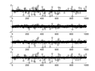
Figure 2: Evolution of SL0 toward the solution: $m=1000$, $n=400$ and $k=100(p=0.1)$. From top to bottom, first plot corresponds to the actual source, second plot is its estimation at the first level ($\sigma=1$), third plot is its estimation at the second level ($\sigma=0.5$), while the last plot is its estimation at third level ($\sigma=0.2$).

The values used for the first part of the experiment are $m=1000$, $n=400$, $p=0.1$, $\sigma_{\mathrm{off}}=0$, $\sigma_{\mathrm{on}}=1$, $\sigma_{n}=0.01$ and the sequence of $\sigma$ is fixed to [1, 0.5, 0.2, 0.1, 0.05, 0.02, 0.01]. $\mu$ is fixed to $2.5$. For each value of $\sigma$ the gradient-projection loop (the internal loop) is repeated three times, i.e., $L=3$ (influence of L is discussed in part of experiment 2; in all other experiments $\mu$ and $L$ are fixed to 2.5 and 3).

We use the CPU time as a measure of complexity. Although it is not an exact measure, it gives a rough estimation of the complexity, for comparing SL0 and LP algorithms. Our simulations are performed in MATLAB7 environment using an AMD Athlon sempron 2400+, 1.67GHz processor with 512MB of memory, and under Microsoft Windows XP operating system.

Table I shows the gradual improvement in the output SNR after each iteration, for a typical run of SL0. Moreover, for this run, the total time and final SNR have been shown for SL0, for LP, and for FOCUSS. It is seen that SL0 performs two orders of magnitude faster than LP, while it produces a better SNR (in some applications, it can be even three orders of magnitudes faster: see Experiment 6). Figure 2 shows the actual source and it’s estimations at different iterations for this run of SL0.

The experiment was then repeated 100 times (with the same parameters, but for different randomly generated sources and mixing matrices) and the values of SNR (in dB) obtained over these simulations were averaged. These averaged SNR’s for SL0, LP, and FOCUSS were respectively 30.85dB, 26.70dB, and 20.44dB; with respective standard deviations 2.36dB, 1.74dB and 5.69dB. The minimum values of SNR for these methods were respectively 16.30dB, 18.37dB, and 10.82dB. Among the 100 runs of the algorithm, the number of experiments for which SNR$>$20dB was 99 for SL0 and LP, but only 49 for FOCUSS.

In the second part of the experiment, we use the same parameters as in the first part, except $\sigma_{\mathrm{off}}=0.01$ to model the noise of the sources in addition to AWG noise modeled by $\sigma_{n}$. The averaged SNR’s for SL0, LP, and FOCUSS were respectively 25.93dB, 22.15dB and 18.24; with respective standard deviations 1.19dB, 1.23dB and 3.94dB.

Experiment 2. Dependence on the parameters

In this experiment, we study the dependence of the performance of SL0 to its parameters. The sequence of $\sigma$ is always chosen as a decreasing geometrical sequence $\sigma_{j}=c\sigma_{j-1},\,1\leq j\leq J$, which is determined by the first and last elements, $\sigma_{1}$ and ${\sigma_{\!J}}$, and the scale factor $c$. Therefore, when considering the effect of the sequence of $\sigma$, it suffices to discuss the effect of these three parameters on the performance. Reasonable choice of $\sigma_{1}$, and also approximate choice of $\mu$ have already been discussed in Remarks 2 to 5 of Section III. Consequently, we are mainly considering the effects of other parameters.

The general model of the sources and the mixing system, given by (39) and (40), has four essential parameters: $\sigma_{\mathrm{on}}$, $\sigma_{\mathrm{off}}$, $\sigma_{n}$, and $p$. We can control the degree of source sparsity and the power of the noise by changing $k=mp$ and $\sigma_{n}$. We examine the performance of SL0 and its dependence to these parameters for different levels of noise and sparsity. In this and in the followings, except Experiment 6, all the simulations are repeated 100 times with different randomly generated sources and mixing matrices and the values of the SNR’s (in dB) obtained over these simulations are averaged.

Figures 3 represents the averaged SNR (as the measure of performance) versus the scale factor $c$, for different values of $k=mp$ and $\sigma_{n}$. It is clear from Fig. 3(a) that SNR increases when $c$ increases form zero to one. However, when $c$ exceeds a critical value (0.5 in this case), SNR remains constant and does not increase anymore.

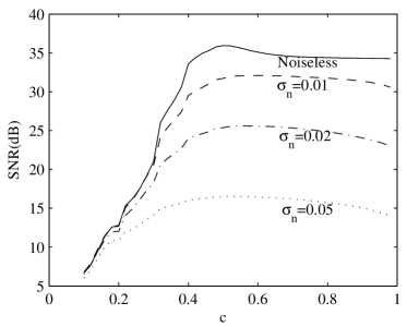
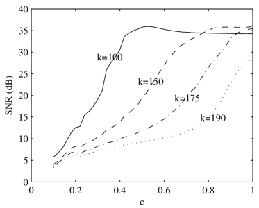
Figure 3: Performance of SL0 as function of $c$ for the case $m=1000$ and $n=400$ (SNR’s are averaged over 100 runs of the algorithm). $\sigma_{1}$ is fixed to 1 (large enough) and ${\sigma_{\!J}}$ is fixed to 0.01 (small enough). In (a) $k$ is fixed to 100 and effect of noise is investigated. In (b) $\sigma_{n}$ is fixed to 0.01 and effect of sparsity factor is analyzed.

Generally, the optimal choice of $c$ depends on the application. When SNR is the essential criterion, $c$ should be chosen large, resulting in a more slowly decreasing sequence of $\sigma$, and hence in a higher computational cost. Therefore, the choice of $c$ is a trade-off between SNR and computational cost. However, as seen in the figures, when $c$ approaches to unity, SNR does not increase infinitely. In Fig. 3(a), the optimal value of $c$, i.e. the smallest value of $c$ that achieves the maximum SNR, is approximatively $c=0.5$. However, it is clear from Fig. 3(b) that the optimal choice of $c$ depends on the sparsity, but not on the noise power. Exact calculation of the optimal $c$ might be very hard. To guarantee an acceptable performance, it suffices to choose $c$ greater than its optimal value.

From [15], we know that $k<n/2$ is a theoretical limit for sparse decomposition. However, most of the current methods cannot approach this limit (see Experiment 3). In Fig. 3(b), $k=190\simeq 200=n/2$ is plotted, and it is clear that by choosing $c$ larger than $0.9$ an acceptable performance can be achieved (however, with a much higher computational cost).

In Fig. 4, SNR is plotted versus $-\ln({\sigma_{\!J}})$ (where ${\sigma_{\!J}}$ is the last and smallest $\sigma$) for different values of $k$ and $\sigma_{n}$. In Fig. 4(a), for the noiseless case, SNR increases linearly, by increasing in $-\ln({\sigma_{\!J}})$. Although not directly clear from the figure, calculation of the obtained values of the figure better shows this linear relationship. This confirms the results of Theorem 1 (accuracy is proportional to the final value of $\sigma$). In the noisy case, SNR increases first, and then remains constant. As was predicted by Theorem 3, in the noisy case the accuracy is bounded and might not be increased arbitrarily.

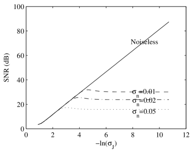
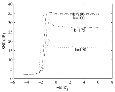
Figure 4: Performance of SL0 versus ${\sigma_{\!J}}$ for $m=1000$ and $n=400$ (SNR’s are averaged over 100 runs of the algorithm). $\sigma_{1}$ is fixed to 1 (large enough) and $c$ is fixed to 0.8 (near enough to one). In (a) $k$ is fixed to 100 and effect of noise is investigated. In (b) $\sigma_{n}$ is fixed to 0.01 and effect of sparsity factor is analyzed.

Generally, the optimal choice of ${\sigma_{\!J}}$ depends on the application. In applications in which SNR is highly more important than the computational load, ${\sigma_{\!J}}$ should be chosen small, resulting in a larger sequence of $\sigma$, and hence a higher computational cost. However, excessively small choice of ${\sigma_{\!J}}$ (smaller than the optimal choice) does not improve SNR (in fact SNR is slightly decreased. Recall also the Remark 6 of Section III). It is clear from Fig. 4 that the optimal choice of ${\sigma_{\!J}}$ depends on the noise power, but not on the sparsity. Exact calculation of the optimal ${\sigma_{\!J}}$ might be very hard. To guarantee an acceptable performance, it suffices to choose ${\sigma_{\!J}}$ less than its optimal value.

From this experiment it can be concluded that, although finding optimal values of the parameters for optimizing the SNR with the least possible computational cost may be very hard, the algorithm is not very sensitive to the parameters, and it is not difficult to choose a sequence of $\sigma$ (i.e., $c$ and ${\sigma_{\!J}}$).

Finally, to study the effect of $L$ (number of iterations of the internal steepest ascent loop), the parameters are fixed to the values used at the beginning of Experiment 1, and the averaged SNR (over 100 runs of the algorithm) is plotted versus $L$ in Fig. 5. It is clear from this figure that the final SNR achieves its maximum for a small $L$, and no longer improves by increasing it, while the computation cost is directly proportional to $L$. Hence, as it was said in Remark 1 of Section III and Remark 3 of Section IV-A, we generally fix $L$ to a small value, say $L=3$.

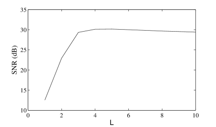
Figure 5: Averaged SNR (on 100 runs of the algorithm) versus $L$ for the case $m=1000$ and $n=400$, $k=100$ and $\sigma_{n}=0.01$

Experiment 3. Effect of sparsity on the performance

How much sparse a source vector ${\bf s}$ should be to make its estimation possible using our algorithm? Here, we try to answer this question experimentally. As mentioned before, there is the theoretical limit of $n/2$ on the maximum number of active sources to insure the uniqueness of the sparsest solution. But, practically, most algorithms cannot achieve this limit [15, 13].

To be able to measure the effect of sparsity, instead of generating the sources according to the model (39), we randomly activate exactly $k$ elements out of $m$ elements. Figure 6 then shows the output SNR versus $k$, for several values of $c$, and compares the results with LP. Note that SL0 outperforms LP, specially in cases where $k\simeq n/2=200$.

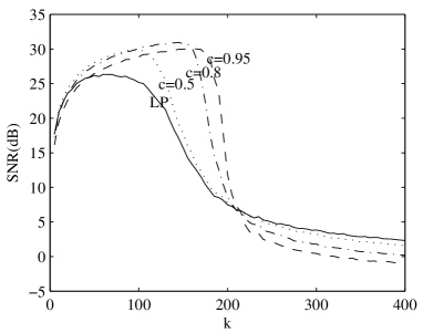
Figure 6: Averaged SNR’s (over 100 runs of the algorithm) versus $k$, the average number of active sources, for SL0 algorithm with several values of $c$, and for LP. The parameters are $m=1000$, $n=400$, $\sigma_{1}=1$, ${\sigma_{\!J}}=0.01$, $\sigma_{n}=0.01$.

It is obvious from the figure that all methods work well if $k$ is smaller than a critical value, and they start breaking down as soon as $k$ exceeds this critical value. Figure 6 shows that the break-down value of $k$ for LP and for SL0 with $c=0.5$ is approximately 100 (half of the theoretical limit $n/2=200$). For $c=0.8$ and $c=0.95$, this break-down value is approximately 150 and 180. Consequently, with our algorithm, it is possible to estimate less sparse sources than with LP algorithm. It seems also that by pushing $c$ toward 1, we can push the breaking-down point toward the theoretical limit $n/2$; however, the computational cost might become intolerable, too.

Experiment 4. Robustness against noise

In this experiment, the effect of the noise variance, $\sigma_{n}$, on the performance is investigated for different values of ${\sigma_{\!J}}$ and is compared with the performance of LP. Figure 7 depicts SNR versus $\sigma_{n}$ for different values of ${\sigma_{\!J}}$ for both methods. The figure shows the robustness of SL0 against small values of noise. In the noiseless case ($\sigma_{n}<.02$), LP performs better (note that $\sigma_{\mathrm{off}}=0$, and in SL0, $\sigma$ is decreased only to 0.005). In the noisy case, smoothed-$\ell^{0}$ achieves better SNR. Note that the dependence of the optimal ${\sigma_{\!J}}$ to $\sigma_{n}$ is again confirmed by this experiment.

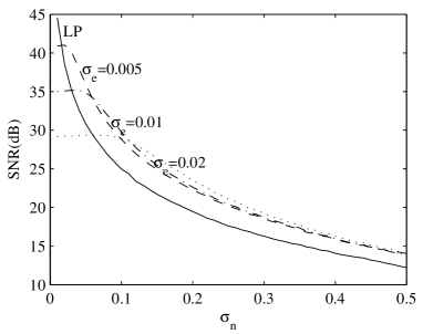
Figure 7: Averaged SNR’s (over 100 runs of the algorithm) versus the noise power $\sigma_{n}$ for different values of ${\sigma_{\!J}}$, and for LP. The parameters are $m=100$, $n=400$, $k=100$, $\sigma_{1}=1$, and $c=0.8$.

Experiment 5. Number of sources and sensors

In this experiment, we investigate the effect of the system scale (i.e., the dimension of the mixing matrix, $m$ and $n$) on the performance and justify the scalability of SL0.

First, to analyze the effect of the number of mixtures ($n$), by fixing $m$ to 1000, SNR is plotted versus $n$, for different values of $k$ in Fig. 8(a). It is clear from this figure that both methods perform poorly while $2k>n$ (note that the sparsest solution is not necessarily unique in this case). SL0 performs better as soon as $n$ exceeds $2k$ (the theoretical limit for the uniqueness of the sparsest solution).

Then, to analyze the effect of scale, $n$ is fixed to $\lceil 0.4m\rceil$, and SNR is plotted versus $\log(m)$ for different values of $k$ in Fig. 8(b). From this figure it is obvious that SL0 and LP perform similarly for small values of $k$ ($k\simeq 10)$, but SL0 outperforms LP for larger values of $k$ ($k\simeq 100$).

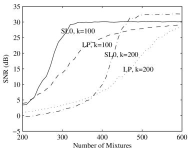
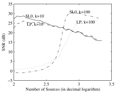
Figure 8: Effect of scale on performance (SNR’s are averaged over 100 runs of the algorithm). $\sigma_{n}=0.01$, $c=0.8$, $\sigma_{1}=1$, ${\sigma_{\!J}}=0.01$, and SL0 is compared with LP. In (a) $m$ is fixed to 1000 and SNR is plotted versus $n$ for different values of $k$. In (b) SNR is plotted versus $\log(m)$ for different values of $k$, while $n$ is fixed to $\lceil 0.4m\rceil$.

Experiment 6. Computational Cost in BSS applications

In BSS and SCA applications, the model (40) is written as ${\bf x}(t)={\bf A}{\bf s}(t)+{\bf n}(t),\,1\leq t\leq T$, where $T$ is the number of samples. In matrix form, this can be written as ${\bf X}={\bf A}{\bf S}+{\bf N}$, where ${\bf X}$, ${\bf S}$, and ${\bf N}$ are respectively $n\times T$, $m\times T$ and $n\times T$ matrices, where each column stands for a time sample.

For solving this problem with LP, the system ${\bf x}(t)={\bf A}{\bf s}(t)+{\bf n}(t)$ should be individually solved for each value of $1\leq t\leq T$. This trivial approach can also be used with SL0. However, since all the steps of SL0 presented in Fig. 1 are in matrix form, it can also be directly run on the whole matrices ${\bf X}$ and ${\bf S}$. Because of the speed of the current matrix multiplication algorithms, this results in an increased speed in the total decomposition process.

Figure 9 shows the average computation time per sample of SL0 for a single run of the algorithm, as a function of $T$ for the case $m=1000$, $n=400$ and $k=100$. The figure shows that by increasing $T$, average computation time first increases, then decreases and reach to a constant. For $T=1$, the computation time is 266ms (this is slightly different with the time of the first experiment, 227ms, because these are two different runs). However, for $T=10000$, the average computation time per sample decreases to 38ms. In other words, in average, SL0 finds the sparse solution of a linear system of 400 equations and 1000 unknowns just in 38ms (compare this with 30s for $\ell_{1}$-magic, given in Experiment 1).

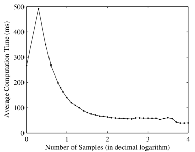
Figure 9: Average computation time per sample of SL0, as a function of $T$, number of (time) samples, for the case $m=1000$, $n=400$ and $k=100$. $\sigma_{n}$ is chosen 0.01 and the sequence of $\sigma$ is fixed to [1, 0.5, 0.2, 0.1, 0.05, 0.02, 0.01], the same parameter used in first experiment.

VI Conclusions

In this paper, we showed that the smoothed $\ell^{0}$ norm can be used for finding sparse solutions of an USLE. We showed also that the smoothed version of the $\ell^{0}$ norm not only solves the problem of intractable computational load of the minimal $\ell^{0}$ search, but also results in an algorithm which is highly faster than the state-of-the-art algorithms based on minimizing the $\ell^{1}$ norm. Moreover, this smoothing solves the problem of high sensitivity of $\ell^{0}$ norm to noise. In another point of view, the smoothed $\ell^{0}$ provides a smooth measure of sparsity.

The basic idea of the paper was justified by both theoretical and experimental analysis of the algorithm. In the theoretical part, Theorem 1 shows that SL0 is equivalent to $\ell^{0}$-norm for a large family of functions $f_{\sigma}$. Theorem 2 gives a strong assessment for using $\ell^{2}$-norm solution for initialization. This theorem also suggests that the minimal $\ell^{2}$ norm can be seen as a rough estimation of the sparse solution (like Method Of Frames), which will be modified in the future iterations. Theorem 3 justifies the robustness of SL0 against noise.

Other properties of the algorithm were studied experimentally. In particular, we showed that (1) the algorithm is highly faster than the state-of-the-art LP approaches (and it is even more efficient in SCA applications), (2) choosing suitable values for its parameters is not difficult, (3) contrary to previously known approaches it can work if the number of non-zero components of ${\bf s}$ is near $n/2$ (the theoretical limit for the uniqueness of the sparse solution), and (4) the algorithm is robust against noise.

Up to now, we have no theoretical result for determining how much ‘gradual’ we should decrease the sequence of $\sigma$, and it remains an open problem for future works. Some open questions related to this issue are: Is there any sequence of $\sigma$ which guaranties escaping from local maxima for the Gaussian family of functions $F_{\sigma}$ given in (1)? If yes, how to find this sequence? If not, what happens with other families of functions $F_{\sigma}$? Moreover, is there any (counter-)example of ${\bf A}$, ${\bf s}$ and ${\bf x}$ for which we can prove that for any sequence $\sigma$ the algorithm will get trapped into a local maximum? These issues, mathematically difficult but essential for proving algorithm convergence, are currently investigated. However, Experiment 2 showed that it is fairly easy to set some parameters to achieve a suitable performance. Moreover, for an estimation ${\bf\hat{s}}$ of the sparsest source (obtained by any method), we provided in Remark 5 of Section IV-A an upper bound for the estimation error.

In addition, future works include better treatment of the noise in the model (40) by taking it directly into account in the algorithm (e.g. by adding a penalty term to $F_{\sigma}$). Moreover, testing the algorithm on different applications (such as compressed sensing) using real-world data is under study in our group.

References

- [1] R. Gribonval and S. Lesage, “A survey of sparse component analysis for blind source separation: principles, perspectives, and new challenges,” in Proceedings of ESANN’06, April 2006, pp. 323–330.
- [2] P. Bofill and M. Zibulevsky, “Underdetermined blind source separation using sparse representations,” Signal Processing, vol. 81, pp. 2353–2362, 2001.
- [3] P. G. Georgiev, F. J. Theis, and A. Cichocki, “Blind source separation and sparse component analysis for over-complete mixtures,” in Proceedinds of ICASSP’04, Montreal (Canada), May 2004, pp. 493–496.
- [4] Y. Li, A. Cichocki, and S. Amari, “Sparse component analysis for blind source separation with less sensors than sources,” in ICA2003, 2003, pp. 89–94.
- [5] S. S. Chen, D. L. Donoho, and M. A. Saunders, “Atomic decomposition by basis pursuit,” SIAM Journal on Scientific Computing, vol. 20, no. 1, pp. 33–61, 1999.
- [6] D. L. Donoho, M. Elad, and V. Temlyakov, “Stable recovery of sparse overcomplete representations in the presence of noise,” IEEE Trans. Info. Theory, vol. 52, no. 1, pp. 6–18, Jan 2006.
- [7] D. L. Donoho, “Compressed sensing,” IEEE Transactions on Information Theory, vol. 52, no. 4, pp. 1289–1306, April 2006.
- [8] R. G. Baraniuk, “Compressive sensing,” IEEE Signal Processing Magazine, vol. 24, no. 4, pp. 118–124, July 2007.
- [9] E. J. Candès and T. Tao, “Decoding by linear programming,” IEEE Transactions Information Theory, vol. 51, no. 12, pp. 4203–4215, 2005.
- [10] M. A. T. Figueiredo and R. D. Nowak, “An EM algorithm for wavelet-based image restoration,” IEEE Transactions on Image Processing, vol. 12, no. 8, pp. 906–916, 2003.
- [11] M. A. T. Figueiredo and R. D. Nowak, “A bound optimization approach to wavelet-based image deconvolution,” in IEEE Internation Conference on Image Processing (ICIP), August 2005, pp. II–782–5.
- [12] M. Elad, “Why simple shrinkage is still relevant for redundant representations?,” IEEE Transactions on Image Processing, vol. 52, no. 12, pp. 5559–5569, 2006.
- [13] I. F. Gorodnitsky and B. D. Rao, “Sparse signal reconstruction from limited data using FOCUSS, a re-weighted minimum norm algorithm,” IEEE Transactions on Signal Processing, vol. 45, no. 3, pp. 600–616, March 1997.
- [14] D. L. Donoho and M. Elad, “Maximal sparsity representation via minimization,” the Proc. Nat. Aca. Sci., vol. 100, no. 5, pp. 2197–2202, March 2003.
- [15] D. L. Donoho, “For most large underdetermined systems of linear equations the minimal -norm solution is also the sparsest solution,” Tech. Rep., 2004.
- [16] I. Daubechies, M. Defrise, and C. DeMol, “An iterative thresholding algorithm for linear inverse problems with a sparsity constraint,” Communications on Pure and Applied Mathematics, vol. 57, no. 11, pp. 1413–1457, 2004.
- [17] E.J. Candès, J. Romberg, and T. Tao, “Robust uncertainty principles: exact signal reconstruction from highly incomplete frequency information,” IEEE Transactions on Information Theory, vol. 52, no. 2, pp. 489–509, February 2006.
- [18] A. Hyvarinen, J. Karhunen, and E. Oja, Independent Component Analysis, John Wiley & Sons, 2001.
- [19] Andrzej Cichocki and Shun-ichi Amari, Adaptive Blind Signal and Image Processing: Learning Algorithms and Applications, John Wiley and sons, 2002.
- [20] F. Movahedi, G. H. Mohimani, M. Babaie-Zadeh, and Ch. Jutten, “Estimating the mixing matrix in sparse component analysis (SCA) based on partial k-dimensional subspace clustering,” Neurocomputing, vol. 71, pp. 2330–2343, 2008.
- [21] Yoshikazu Washizawa and Andrzej Cichocki, “On-line k-plane clustering learning algorithm for sparse comopnent analysis,” in Proceedinds of ICASSP’06, Toulouse (France), 2006, pp. 681–684.
- [22] Y.Q. Li, A. Cichocki, and S. Amari, “Analysis of sparse representation and blind source separation,” Neural Computation, vol. 16, no. 6, pp. 1193–1234, 2004.
- [23] M. Zibulevsky and B. A. Pearlmutter, “Blind source separation by sparse decomposition in a signal dictionary,” Neural Computation, vol. 13, no. 4, pp. 863–882, 2001.
- [24] S. Mallat and Z. Zhang, “Matching pursuits with time-frequency dictionaries,” IEEE Trans. on Signal Proc., vol. 41, no. 12, pp. 3397–3415, 1993.
- [25] E. Candes and J. Romberg, “-magic: Recovery of sparse signals via convex programming,” 2005, URL: www.acm.caltech.edu/l1magic/downloads/l1magic.pdf.
- [26] S. Krstulovic and R. Gribonval, “MPTK: Matching pursuit made tractable,” in ICASSP’06, Toulouse, France, May 2006, vol. 3, pp. 496–499.
- [27] A. A. Amini, M. Babaie-Zadeh, and Ch. Jutten, “A fast method for sparse component analysis based on iterative detection-projection,” in AIP Conference Proceeding (MaxEnt2006), 2006, vol. 872, pp. 123–130.
- [28] G. H. Mohimani, M. Babaie-Zadeh, and C. Jutten, “Fast sparse representation based on smoothed l0 norm,” in Proceedings of ICA’07, LNCS 4666, London, UK, September 2007, pp. 389–396.
- [29] G. H. Mohimani, M. Babaie-Zadeh, and C. Jutten, “Complex-valued sparse representation based on smoothed norm,” in Proceedings of ICASSP2008, Las Vegas, April 2008, pp. 3881–3884.
- [30] A. Blake and A. Zisserman, Visual Reconstruction, MIT Press, 1987.