Getting in the Zone for Successful Scalability

1 INTRODUCTION

The 2008 JavaOne conference included many presentations on techniques for achieving better scalability, e.g., caching, collocation, “parallelization,” and pooling. But these are only qualitative descriptions. How can the impact of applying such techniques be quantified? Clearly, this is the domain of performance modeling. Performance models are essential, not only for prediction, but also for interpreting scalability measurements. However, most performance modeling tools, e.g., PDQ [Gun 05] and SIMUL8 [Hol04b ], use a queueing paradigm which requires measured service times as inputs to parameterize each queueing facility being modeled. More often than not, such detailed measurements are not available, thereby thwarting this approach.

A more practical approach is based on statistical regression [Hol04a ] of measured throughput data using parametric models; the advantage being that service-time measurements are not required. One parametric model that has been used successfully for the past two decades is based on the universal scalability law or USL Gun [93, 07, 08]. A distinguishing feature of the USL is its ability to analytically model the retrograde throughput (Fig. 1) commonly seen in custom benchmarks and load-test measurements. If such retrograde behavior is not present, the USL reduces to either Amdahl’s law (See Sect. 2.2) or Gustafson’s linearized form (See Sect. 2.3).

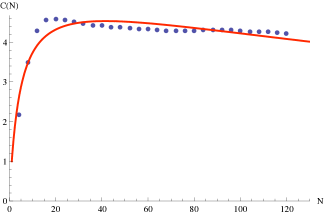
Figure 1: USL parametric model (red) fitted to Websphere relative capacity measurements $C(N)$ as a function of user load $N$ with coefficients $\alpha=0.18169$ and $\beta=0.00047$. Retrograde performance is clear. Amdahl and Gustafson parametric models cannot accommodate this effect

.

As useful as all this has been, the question has remained: Do parametric models like USL represent something more fundamental? We answer that question in the affirmative by showing that the USL corresponds to a certain bounding curve on the throughput of a machine repairman (MRM) queueing model [GH 98]. We use event-based simulation as an exploratory tool to investigate the precise conditions under which such a bound can exist. Amdahl’s law and Gustafson’s linearization are contained as special cases of the MRM model. Based on this new insight, we introduce the concept of scalability zones. Rather than relying on any particular bounding curve to express scalability, we show how each of these bounding curves defines a set of zones. In practice, typical throughput measurements lie across all these zones and this provides a more helpful interpretation for determining potential performance improvements.

Our paper is organized as follows. In Sect. 2 we review each of the parametric scalability models discussed subsequently. In Sect. 3 we review the repairman model and the generalizations necessary to make contact with the parametric models. These extensions include: (i) a prepping repairman in Sect. 3.2 and (ii) synchronous queueing in Sect. 3.3. Sect. 4 describes the simulation models and presents the results that support the identification of the USL with synchronous queueing at a prepping repairman, together with several special cases. Finally, in Sect. 5, we discuss a new approach to interpreting scalability data in terms of zones and transitions between them. These zones are well-defined in terms of queueing effects and thus, can provide vital insights into how best to improve scalability. An example of applying the zone concept to actual scalability measurements is presented.

2 PARAMETRIC MODELS

We begin our analysis by defining the relative capacity:

$$C(N)=X(N)/X(1)$$ (1)

where $X(N)$ represents the throughput generated by either, $N$ processors in the case of hardware scalability [See Gun 07, Chap. 4] or $N$ virtual users in the case of software scalability [See Gun 07, Chap. 6]. The ratio in (1) has two possible interpretations:

Data representation:

$X(N)$ represents the actual throughput measurements, e.g., transactions per second. The relative capacity $C(N)$ is simply the normalization of those data. See Fig. 1.

Analytic representation:

$X(N)$ is represented by a function, e.g., a linear regression model such as: $X(N)=mN+c$ where $m$ is the slope and $c$ is the intercept. See Sect. 4.4

With regard to each of the parametric models discussed in this section, we shall demonstrate that $C(N)$ is best represented, not by a simple linear function, but by a ratio of functions:

$$C(N)=P(N)/Q(N)$$ (2)

where $P(N)$ and $Q(N)$ are polynomials in $N$. Such functions are called rational functions (See en.wikipedia.org/wiki/Rational_function).

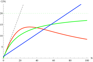
Figure 2: Parametric models: USL (red), Amdahl (green), Gustafson (blue), with parameter values exaggerated to distinguish their typical characteristics relative to ideal linearity (dashed black). The horizontal dashed green line is the Amdahl asymptote at $\alpha^{-1}$. Compare with the application of the USL model in Fig. 1

.

We pause to reflect on the significance of (2). Computer system scalability can be modeled using many possible functions which are not rational functions, e.g., geometric scaling [Gun 96]. As we shall show in Sects. 3 and 4, rational functions are physically correct because they possess a deep connection with queueing theory. As far as we are aware, this fundamental relationship between parametric models and queueing models has not been elucidated before. Conversely, geometric scaling can be excluded on the grounds that it is unphysical from the standpoint of queueing theory [Gun 07, 02].

2.1 Universal Scalability Law

The most general parametric model of scalability is the two-parameter universal scalability law (USL):

$$C(N,\alpha,\beta)=\dfrac{N}{1+\alpha(N-1)+\beta N(N-1)}$$ (3)

which is a rational function with $P(N)=N$ and $Q(N)=aN^{2}+bN+c$; a quadratic polynomial with coefficients $a,b,c\geq 0$. These coefficients have been regrouped into three terms involving only two parameters $\alpha,\beta\geq 0$, in the denominator of (3). These three terms can be interpreted as the “Three C’s”:

1. Concurrency-limited scalability when $\alpha,\beta=0$ such that $C(N)\sim N$, i.e., linear scaling.

2. Contention-limited scalability due to serialization or queueing, i.e., when $\alpha>0,\beta=0$.

3. Coherency-limited scalability due to the delay incurred by making local copies of data or instructions consistent across multiple caches or nodes, i.e., when $\alpha,\beta>0$.

Table 1 summarizes how these parameter values can be used to classify the scalability of different types of platforms and applications.

Table 1: Application classes for the USL model

	Ideal concurrency ($\alpha,\beta=0$)
	Single-threaded tasks
A	Parallel text search
	Read-only queries
	Contention-limited ($\alpha>0,\beta=0$)
	Tasks requiring locking or sequencing
B	Message-passing protocols
	Polling protocols (e.g., hypervisors)
	Coherency-limited ($\alpha=0,\beta>0$)
	SMP cache pinging
C	Incoherent application state between
	cluster nodes
	Worst case ($\alpha,\beta>0$)
	Tasks acting on shared-writable data
D	Online reservation systems
	Updating database records

2.2 Amdahl’s Law

Amdahl’s law [Amd 67] corresponds to the special case of the USL equation (3) with $\beta=0$. Typically, it is used to quantify the achievable speedup:

$$C_{A}(N,\alpha)=\dfrac{N}{1+\alpha(N-1)}$$ (4)

for fine-grained parallelism. Equation (4) is a rational function with $P(N)=N$ and $Q(N)=bN+c$; a linear polynomial with coefficient values $a,b,c\geq 0$.

Amdahl’s law assumes that a single workload comprises a parallel portion and a remaining serial portion. The serial portion or serial fraction, $0<\alpha<1$, is the aggregate fraction of the workload that can only be executed sequentially on a single processor, i.e., the non-parallel portion.

Another fundamental assumption is that the parallel portion of the workload can be partitioned into $N$ equal sub-tasks. If the size of these sub-tasks can be made progressively smaller, then the elapsed execution time will become dominated by the serial fraction such that $C(N)\sim 1/\alpha$ as $N\rightarrow\infty$. In other words, there is an asymptotic ceiling on achievable speedup shown as the horizontal line in Fig. 2.

2.3 Gustafson’s Linearization

Amdahl’s law assumes the size of the work is fixed. Gustafson’s modification [Gus 88] is based on the idea of scaling up the size of the work to match the $N$ processors [See Gun 07, Chap. 4]. This rescaling of the workload results in the theoretical recovery of linear speedup

$$C_{G}(N,\alpha)=(1-\alpha)N+\alpha$$ (5)

which is a rational function with $P(N)=bN+c$; a linear polynomial with coefficients $a,b,c\geq 0$ and $Q(N)=1$, trivially.

Unlike the USL, (5) exhibits the peculiarity that $C_{G}(0,\alpha)=\alpha$, i.e., there is non-zero capacity even if there are no processors in the system! This artifact is shown as the blue line near the origin in Fig. 2 and must be regarded as an unphysical side-effect of the Gustafson linearization of Amdahl’s law.

Although $C_{G}(N,\alpha)$ has inspired various efforts for improving parallel processing efficiencies, achieving truly linear speedup has turned out to be extremely difficult in practice. Most recently, (5) has been proposed as a way to “break Amdahl” scalability for threaded applications running on multicore processors [Sut 08]. Whether this claim will be effective, remains to be seen. There is a significant literature of failed proposals for defeating Amdahl’s law [See, e.g., KH 92, Nel 96, Pre 95]. See Sect. 5 for some additional remarks based on the results of this paper.

2.4 Retrograde Scalability

The key difference between the USL and the other parametric models lies in the fact that only the USL can successfully predict retrograde scaling. See Fig. 2. In other words, if we think of Gustafson’s linear scalability as corresponding to “equal bang for the buck,” and Amdahl’s law as representing “diminishing returns,” then the USL represents “negative return on investment,” or negative ROI.

Such negative ROI effects in application scalability are not the exception but the norm. Figure 1 shows an example of WebSphere benchmark data fitted using Mathematica. The retrograde effect is manifest. It is in this sense that the USL is considered to be universal.

Theorem 1 (Universality).

The necessary and sufficient condition for the relative capacity $C(N)$ to be a universal scalability model is $P(N)=N$ and $Q(N)=aN^{2}+bN+c$ with coefficients $a,b,c>0$.

Proof 1.

The proof is best demonstrated by considering latency rather than throughput. See [Gun 08] for details of this proof. ∎

Interestingly, the proof establishes a similarity between the USL and Brooks’ law [Bro 95] for the management of software projects, viz., “Adding more manpower to a late software project makes it later.” In this case, $N$ is interpreted as people rather than processes or processors. Brooks’ law is the analog of the negative ROI mentioned earlier.

Equation (3) clearly satisfies theorem 1. Next, we show that each of these parametric models has a more fundamental meaning because they correspond to bounds on throughput for a well-defined queueing model.

3 QUEUEING MODELS

In Sects. 3.2 and 3.3, we develop some generalizations of the MRM that do not appear in the queueing-theory literature. First, we briefly review the standard MRM.

3.1 Standard Repairman

The repairman queueing model [GH 98] is shown schematically in Fig. 3) and represents an assembly line comprising a finite number of machines $p$ which break down after a mean lifetime $Z$. A repairman takes a mean time $S$ to repair each broken machine. If multiple machines fail, the additional machines must queue for service in FIFO order. The queue-theoretic notation for the MRM model, $M/M/1//N$, implies exponentially distributed lifetimes and service periods with a finite population $N$ of requests and buffering.

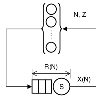
Figure 3: Machine repairman schematic

In steady state, $ZX$ machines are “up”, while $Q$ are “down” for repairs, such that the total number of machines in either state is given by $N=Q+ZX$. Rearranging this expression we have:

$$Q=N-ZX$$ (6)

and applying Little’s law $Q=XR$ to

$$XR=N-ZX$$ (7)

produces

$$R(N)=\dfrac{N}{X(N)}-Z$$ (8)

for the mean residence time at the repair station. Rearranging (8) provides an expression for the mean MRM throughput as a function of $N$:

$$X(N)=\dfrac{N}{R(N)+Z}$$ (9)

Several solutions of $X(N)/X(1)$ are shown in Fig. 4.

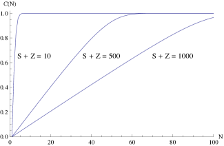
Figure 4: MRM throughput curves with normalized saturation values for round-trip times equal to 10, 500 and 1000 service units. No degradation is possible for any choice of $N$, $S$ or $Z$

MRM has its origins in operations research associated with manufacturing systems [GH 98]. However, because all queueing models are only abstractions, MRM has found more widespread applications. The two most important applications for our discussion are:

Time-share systems:

$N$ represents users making requests to a central processing facility. An MRM queueing model was applied to the performance analysis of a research time-share computing system called CTSS [Sch 67]; the precursor to UNIX.

Multiprocessors:

$N$ represents CPUs or cores and the MRM represents the interconnect that allows the CPUs to communicate and share data [AMBC 90, RF 87].

Table 2: Interpretation of the queueing metrics in Fig. 3 where MRM: machine repairman, CMP: core multiprocessor and TSS: time-share system

Metric	Model	Interpretation
	MRM	machines
$N$	CMP	processors, cores
	TSS	processes, users
	MRM	up time
$Z$	CMP	execution period
	TSS	think time
	MRM	service time
$S$	CMP	transmission time
	TSS	CPU time
	MRM	residence time
$R(p)$	CMP	interconnect latency
	TSS	queueing time
	MRM	failure rate
$X(p)$	CMP	bus bandwidth
	TSS	appln. throughput

A summary of how to interpret the MRM queueing variables in each of the described cases is provided in Table 2. The multiplicity of MRM interpretations justifies the statement in Sect. 2 that these parametric models can be applied to both hardware and software scalability analysis. In particular, since the USL model (3) does not presume any particular type of application or topology, it can be applied equally well from multi-cores to multi-tier systems. That detailed information is present in the USL, but it is encoded in the two parameters: $\alpha$ and $\beta$.

Having reviewed the standard MRM, we new develop some generalizations that will be needed to make the connection between the MRM and the USL explicit. These generalizations are: (i) state-dependent service times and (ii) synchronous queueing, which we treat in Sects. 3.2 and 3.3, respectively.

3.2 Prepping Repairman

Figure 4 shows that the mean throughput is approximately linear for values of $N$ near the origin (i.e., low load) and reaches a saturation plateau at high loads when $N>S/(S+Z)$. Retrograde throughput, of the type exhibited in Fig. 1, is not possible in the standard MRM for any choice of $N$, $S$ or $Z$. However, we do know that retrograde throughput is associated with load-dependent servers in queueing models [See e.g., Gun 05, Chap. 10].

The question then becomes: What should be the form of the load-dependency such that the MRM produces exactly the retrograde throughput exhibited by the USL? In principle, such load-dependence could take any form. In Sects. 3.3 and 4.5 we show, rather surprisingly, that simple linear load-dependence is required to produce USL behavior in the MRM.

Linear load-dependence in the context of the MRM means that the repairman has to prepare up to $N$ failed machines in some way, e.g., rank them, prior to actually servicing them. In general, such ranking will involve pairwise comparisons and this introduces an additional delay that grows binomially with $N$, i.e., $\binom{N}{2}=N(N-1)/2$. Up to a factor of 2, this is precisely the term in the denominator of (3). It is the queueing analog of negative ROI discussed in Sect. 2.4.

It is important to realize that this additional delay due to preparations, is suffered by all of the enqueued machines before the repairman commences service. For brevity, we shall hereafter refer to this kind of load-dependent repairman as the prepping repairman.

3.3 Synchronous Queueing

One more condition is necessary in order to establish the connection between the parametric models of Sect. 2 and the MRM, viz., synchronous queueing. The reason for this requirement stems from the fact that the residence time $R(N)$ in (9) can be quite arbitrary and, mathematically speaking, may not even possess an analytic form. But even if $R(N)$ does have an analytic form, it is unlikely to be a polynomial in $N$ and thus, will not produce rational functions like (2).

If, however, all machines were to break down simultaneously, the queue length at the repairman would be maximized such that the residence time becomes $R(N)=NS$, i.e., one machine in service and $(N-1)$ waiting. Synchronous queueing produces worst-case throughput and it therefore represents a lower bound [ZSEG 82] on (9):

$$\dfrac{N}{NS+Z}\leq X(N)$$ (10)

In the context of multiprocessor scalability (see Table 2), it is tantamount to all $N$ processors simultaneously exchanging data or sending messages across the interconnect.

It is this synchronous queueing condition that causes the throughput (9), in both the standard and load-dependent MRM models, to conform to (2) and thus provide the connection with the rational functions discussed in Sect. 2.

Theorem 2 (Main theorem).

The universal scalability law (3) is equivalent to the synchronous bound on relative capacity in the MRM with linear load-dependent service rate.

Proof 2 (Sketch).

Under synchronous queueing in MRM, when the first request is in service the mean waiting time for the remainder is given by

$$W=(Q-1)\,S$$ (11)

where $Q$ is the mean number of requests in the system. Now, let the service time be load-dependent such that:

$$S(Q)=c\,QS$$

with $c$ a constant of proportionality. For synchronous queueing $Q\equiv N$, so we can rewrite (11) as:

$$W=c\,(Q-1)\,QS=c\,N\,(N-1)\,S$$ (12)

Expressed as relative relative throughput, (12) appears in the denominator of (3) as the $N(N-1)$ term. The detailed proof appears in [Gun 08]. ∎

If we consider synchronous queueing in the standard MRM, i.e., without load-dependent service, we recover Amdahl’s law, which is also the special case of USL with $\beta=0$ in (3).

Corollary 1.

Amdahl’s law (4) is equivalent to the relative throughput due to synchronous queueing in the standard MRM with mean execution time $Z$ and constant service rate $S$.

Proof 3.

The proof requires the identity

$$\alpha=\frac{S}{S+Z}\,.$$ (13)

See [Gun 07, Appendix A] and [Gun 02] for details. ∎

Corollary 2.

Gustafson’s law (5) corresponds to the rescaling $Z\mapsto pZ$ in the MRM.

Proof 4.

See [Gun 08] as well as the simulation results in Sect. 4.4.

The precise nature of the synchronization discussed here turns out to be rather subtle. To see this, consider the case where all $N$ machines have the same deterministic $Z$ period. At the end of the first $Z$ period, all $N$ machines will enqueue at the MRM simultaneously. By definition, however, the machines are serviced serially, so they will return to the the operational phase (parallel execution in the top portion of Fig. 3) separately and thereafter will always return to the repairman at different times. In other words, even if the queueing system is started with synchronized visits to the repairman, that synchronization is immediately lost after the first tour because it is destroyed by the very process of queueing.

Unfortunately, the analytic equations used in this section only provide a steady-state view of the MRM, so we cannot discern the details of the stable synchronization process. Consequently, we turn to discrete-event simulation models [Hol04b ] as an exploratory tool, rather than a predictive tool. As we shall see in Sect. 5, the synchronous MRM simulations also provide deeper insight into potential performance tuning opportunities in real systems.

4 SIMULATION MODELS

From a basic modeling standpoint, using discrete event simulation, these look relatively the same with a fixed number of requests circulating through a closed system with a wait time and service time associated with them. The basic model is shown in Fig. 5.

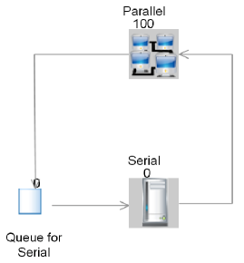
Figure 5: SIMUL8 model corresponding to Fig. 3

There is a place where the requests are running in parallel on multiple CPUs, and another place where the requests are serialized on a single CPU. The cases differ in how requests make the transitions between the two modes of operation.

The simulation models are intended to clarify how the analytical results in Sects. 2 and 3 relate to the way an actual application executes. (cf. Fig. 1) They will be used to demonstrate what features of an architecture might drive an application to the various performance regions or zones defined in Fig. 15. Some of us might be mathematically challenged and prefer to see something running on a real platform, on which we can measure performance, that exhibit the characteristics defined by the analytical equations. In lieu of a real platform, we use simulation models. The criteria used in each of the models on how the parameters are used and how they related to the real world will be defined. Hopefully this will provide the reader with a better understanding of how each of these models are representative of situations that they might have seen on their own computer systems.

We have presented a number of mathematical equations that represent the expected throughput of various models of computer scalability. There are four models discussed in this section for which a discrete simulation queueing model will be created to show that there is a correlation between what the analytic models predict and the results of the simulation models (and thus real platforms).

Discrete event simulation can be defined as “the operation of a system is represented as a chronological sequence of events. A common exercise in learning how to build discrete-event simulations is to model a queue, such as customers arriving at a bank to be served by a teller. In this example, the system entities are CUSTOMER-QUEUE and TELLERS.” As mentioned in Sect. 1, this approach has been used to create models for computer performance evaluation. Simulation represents a real system by modeling the important characteristics. For the models in this paper, there are three objects that are used in the modeling:

1. Resource to be consumed (CPU cycles in this case)

2. Consumer of the resource (CPU actively working on a request)

3. Queue to hold requests for the CPU if it is not available

A word of clarification might be helpful in light of the comment made in Sect. 1, regarding the common impass of needing to parameterize queueing models with service times that are often not available in standard performance measurements. We are not using simulation models to make performance predictions in the usual sense. The simulation models discussed in this paper are constructed to explore the underlying dynamics of the analytic scalability models in Sect. 2 and 3. In order to reveal the connection between the simulation models and the analytic models, it turns out that we only need to define the ratios between the queueing variables $N$, $S$ and $Z$ in Table 2. The actual numbers can be any numeric values, e.g., $S=1.0$ second. In this sense, we are free to construct our simulation models because they do not require measured service times.

4.1 Repairman Simulation

The first simulation model we consider is the standard MRM defined in Sect. 3.1. This model is a closed queueing model and can be used to explain the performance of a system where jobs can run in parallel (no contention for the CPU resource), but every so often they enter a serial activity where only one request can be processed at a time (e.g., programs requesting a lock on a common table). In this case multiple requests may queue up waiting to progress through the serial portion. The other characteristic of the MRM is that it is also defined as an asynchronous model in that the jobs may enter the serial portion independent of one another.

This model (Fig. 5) was constructed using the SIMUL8 event-based simulator. Here the flow of work in closed system is represented. As soon as the serial portion is completed, the request can start execution in parallel with other requests. The “Serial” (S) and “Parallel” (P) objects are consumers of the “CPU” resource, which in this case has 100 CPUs available so that all 100 requests can execute at the same time in the Parallel object. The Serial object has the restriction that only one CPU can be used at a time, forcing outstanding requests to be queued and processed sequentially.

Besides the number of CPUs, the other important parameter in the model in the percent of CPU time spent in the serial execution as compared to the parallel execution. For all the models in this paper, 10% of the time is serial operation. If the time to process a unit of work is 1 second, then $0.9$ seconds are spent in the parallel path and 0.1 seconds in the serial path. The bottleneck of the system is the serial path and will limit the throughput to 10 jobs per second ($1/0.1$). In the model the timings in the Parallel and Serial objects are an exponential distribution based on the service time given above.

So what we want to do in the model is to run a series of configurations and measure the throughput of the system. In this case the percentage in the serial path is fixed and the number of initial requests is varied. The number of available CPUs is set to the number of initial requests. The throughput will be normalized to a system with a single request. Plotting this curve will provide an indication of the effect of adding more CPUs to handle the load as the number of requests in the system also increases. Fig. 6 is the result of the model using the percentages above.

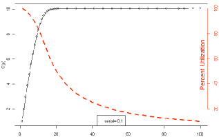
Figure 6: Throughput of the conventional MRM

The x-axis presents the number of CPUs (or requests) in the system. As you can see, we reach a normalized throughput of 10 relatively quickly. Plotted on the secondary y-axis on the right is the system utilization as would be measured by the operating system. Notice that when we reach 100 CPUs, the overall system utilization is only 10%, or as indicated by the graph, only 10 CPUs are doing useful work; the other are idle since the tasks that were executing on them are in the queue waiting for serial execution.

From Table 2, we know that the MRM is representative of a multi-user ($N$), client/server, system where asynchronous requests are contending for a common resource. To minimize loss of throughput, the serial portion must be reduced or the work partitioned so the CPUs can be used more effectively.

The model can provide the direct numbers in the case of the MRM (e.g., an average of $89.7$ requests in the queue and a response time of $9.07$ seconds for a request to make it through the serial portion). But we will see in the other models we will not be able to directly measure these values because of the way the model handles the synchronization of the Parallel and Serial operation. But we can derive these values by keeping track of the amount of CPU consumed in the Parallel and Serial components.

For the case of the MRM with $N=100$ requests, the model was run for $3,000$ seconds, and $27,206$ CPU seconds were consumed in Parallel and $2,999$ in the Serial object. There were $30,118$ requests processed in this time. We can also determine the average number of requests by evaluating the number of CPU sec/sec consumed, which will indicate the number of CPUs required to handle the requests.

$$N_{P} =\dfrac{27206~{}\text{CPU}}{3000~{}\text{sec}}=9.07~{}~{}\text{CPU sec/sec}$$

$$N_{S} =\dfrac{2999~{}\text{CPU}}{3000~{}\text{sec}}=1.00~{}~{}\text{CPU sec/sec}$$

We have the number of requests in the Parallel and Serial objects, so therefore the remainder must be in the queue for the Serial object:

$$N_{Q}=100-9.07-1.00=89.93$$

The response time can be computed using Little’s law:

$$R=\dfrac{N_{Q}+N_{S}}{X}=\dfrac{89.93+1.00}{30118/3000}=9.06~{}\text{sec}$$

where $X$ is the throughput of the MRM.

4.2 Synchronization Gate

The difference between the MRM and Amdahl models is the way that work is returned to the parallel/think processing node. In standard MRM, you can imagine the repairman being presented with a bin of parts that need so have service done on them before returning to operation. The repairman will take a part out of the “bin,” do something to it for time $S$, and then return the part back into operation before picking out the next one from the bin.

In the case of Amdahl, the repairman will still receive a bin of parts to service, but instead of immediately returning the part to operation after it has been serviced, the repairman put the part in an output bin and only when the input bin has been completely serviced are all the parts returned to operation. As shown in Fig. 7, there is effectively a “gate” that prevents the release of parts until the repairman has repaired all of them.

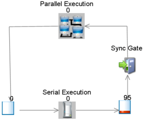
Figure 7: MRM with synchronization gate

Only after all the jobs were in the right buffer after the serial execution were they released back to the parallel execution. But this had some problems in that in the real world jobs do not necessarily all stop at the same time and request some serial operation. There were also some limitations on the types of distributions that could be used for the serial and parallel timings. To overcome these limitations, consider a time sharing system where is one of the jobs needs to run on the serial path, it will stop or suspend all the jobs on the parallel path until it completes. That is effectively what the gate is doing in the figure above. The only impact on the parallel jobs is that their elapsed time has been increased by the time it took the serial job to execute. With this approach, jobs can come out of the parallel path in a random fashion and the overall effect is the same as using a gate.

So the new model of the system looks like Fig. 8 where as soon as a job starts execution on the serial path, a suspend signal is sent to the parallel portion (could be on the next clock tick all the jobs are put in a suspended mode). The serial job will execute and when it is complete, the suspended jobs will be restarted and the job that completed the serial path is returned to execute in the parallel path.

4.3 Amdahl Simulation

Figure 8 is very similar to the MRM (Fig. 5) with the exception that if there is a request running in the Serial object, the processing in the Parallel object will be suspended for the duration of the Serial execution. This is equivalent to all the requests trying to get at the same resource at the same time and each one is serialized and none can restart until all the serial requests have been handled.

In the simulation model, when a request starts to operate in the Serial object, a “breakdown” will be generated for the Parallel object. All work will stop (be suspended) in the Parallel object for the duration of execution on the Serial object and will then pick up where they left off. This effectively extends the elapsed time in Parallel, but the CPU time stays the same. This is contrasted with the MRM, where the elapsed time was the same as the CPU time in the Parallel object.

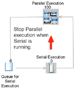
Figure 8: Amdahl model in SIMUL8

In Fig 9, the points represent the output from the model and the green line represents the normalized throughput (speedup) as predicted by Amdahl’s law. The model, which represents a “synchronous” MRM, correlates exactly with the predicted results from Amdahl’s law. The limit in this case is also a speedup of $10$.

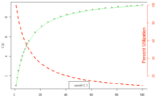
Figure 9: Amdahl throughput

The reason for calculating the number of requests in each object, and the response time, in the following manner is that if you look in the model, the number of requests in the queue averages zero. This is because as soon as a request is completed in the Parallel object, it is sent to the Serial object where it immediately begins execution, since a request can only complete in the Parallel object if it is not suspended which mean there is no request being processed on the Serial object.

This model was run for $3000$ seconds and had a throughput of $27624$ requests. The number of requests in each of the objects and the response times are:

$$N_{P} =\dfrac{24842~{}\text{CPU}}{3000~{}\text{sec}}=8.28~{}~{}\text{CPU sec/sec}$$

$$N_{S} =\dfrac{2750~{}\text{CPU}}{3000~{}\text{sec}}=0.92~{}~{}\text{CPU sec/sec}$$

$$N_{Q} =100-8.28-0.92=90.80$$

$$R =\dfrac{90.80+0.92}{27624/3000}=9.96~{}\text{sec}$$

4.4 Gustafson Simulation

The next simulation model represents Gustafson’s parametric equation discussed in Sect. 2.3. This simulation model (Fig. 10) is similar to the Amdahl model in that requests are running in parallel until they all need the serial portion at the same time, but instead of each request being processed sequentially through the serial portion, all the requests are processed as a batch on a single CPU with a constant service time. This might represent locking on a common table that takes the same time to update, no matter how many requests are waiting. In the Amdahl model, each request must be processed sequentially, so that when there are more requests, there is an additional increase in the time spent in the serial portion. For the Gustafson model, the time spent in the serial portion is constant and is restricted to using a single CPU.

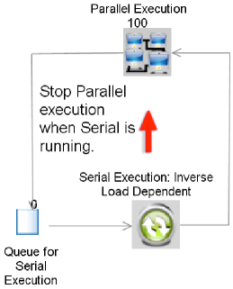
Figure 10: Gustafson model in SIMUL8

Refering to Fig. 11, the speedup is linear (diagonal line). The system utilization (curve) falls from 100% and approaches an asymptote at 90% as $N$ increases. As mentioned in the last paragraph of Sect. 4, this follows from the ratio choice of 10% for the serial fraction defined in (13). The parallel timing is a fixed/constant distribution so that all the requests ask for the serial portion at the same time and the serial timing is exponential.

Gustafson’s law is a linear function; the blue line in Fig. 2. Fitting a linear regression model [Hol04a ] of the form $C(N)=mN+c$ produces $C(N)=0.909N+0.084$ with the coefficient of determination $R^{2}=1$, indicating a nearly perfect fit to the simulation data. To within experimental error the gradient $m=0.909$ represents the gradient in Gustafson’s law, i.e., $(1-\alpha)=0.90$, since we chose $\alpha=0.10$ in all our simulations. Similarly, rounding the intercept value to one significant digit gives $c\simeq 0.1$, in agreement with $\alpha=0.10$ as the intercept in (5).

This model was run for $3000$ seconds and had a throughput of $299608$ requests.

$$N_{P} =\dfrac{270033~{}\text{CPU}}{3000~{}\text{sec}}=90.0~{}~{}\text{CPU sec/sec}$$

$$N_{S} =\dfrac{299~{}\text{CPU}}{3000~{}\text{sec}}=0.10~{}~{}\text{CPU sec/sec}$$

$$N_{Q} =100-90.0-0.10=9.9$$

$$R =\dfrac{9.9+0.10}{299608/3000}=0.10~{}\text{sec}$$

The response time remains the same as the service time ($0.1$ seconds), which is what is expected with the Gustafson model.

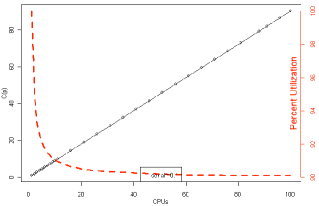
Figure 11: Gustafson throughput

4.5 USL Simulation

The next case is the USL model defined in Sect. 2.1. This is similar to the Amdahl model, but with the addition of a load-dependent serial server. What this means is that as the number of requests waiting for serial service increases, the amount of time that it take the serial portion to run also increases. This is equivalent to a program that might read through the waiting queue to pick the highest priority request to process. So each time a message is retrieved from the queue, the entire queue is searched. This might not take a lot of time, but as the number of outstanding requests increases, so does the serial processing time.

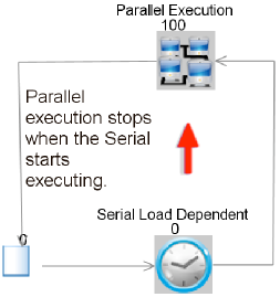
Figure 12: USL model in SIMUL8

This model was run with 10% of the time spent in the serial portion and an additional 0.1% increase in the serial service time for every request that is waiting in the queue.

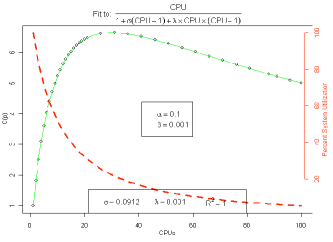
Figure 13: USL throughput

Figure 13 illustrates a retrograde speedup due to the increase in processing time based on the number of requests outstanding in the queue. The points on the graph are the output from the simulation model. The green line is a fit to the Universal Scalability equation. The legend at the bottom of the graph is output from fitting the data points to the equation. The results from the model match the equation ($R^{2}=1$), indicating that Universal Scalability is the equivalent of an Amdahl model, with the addition of a load-dependent serial server.

The model was run for $3000$ seconds and had a throughput of $14727$ requests.

$$N_{P} =\dfrac{13245~{}\text{CPU}}{3000~{}\text{sec}}=8.28~{}~{}\text{CPU sec/sec}$$

$$N_{S} =\dfrac{2867~{}\text{CPU}}{3000~{}\text{sec}}=0.92~{}~{}\text{CPU sec/sec}$$

$$N_{Q} =100-4.42-0.96=94.62$$

$$R =\dfrac{94.62+0.96}{14727/3000}=19.47~{}\text{sec}$$

4.6 Generalized Distributions

For the simulations in Sect. 4, exponential distributions were used in all cases since they are the basis for solving most analytical equations. See Sect. 3.1. But we can show with the simulation models that any distributions can be chosen for the service times, thereby extending the applicability of the USL.

Figure 14 shows the USL model run with the Parallel service time deterministic (FIXED 0.9) and the Serial service time a normal distribution (NORMAL(0.1, 0.02), i.e., a mean of $0.1$ and a standard deviation of $0.02$. The result is very similar to Fig. 13.

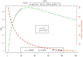
Figure 14: USL model with generalized distributions

5 SCALABILITY ZONES

The simulation results presented in the previous section, not only verify theorem 2 for the USL, but they also provide a deeper insight into the nature of the “Three C’s” in Sect. 2.1. In fact, we could reinterpret them as follows:

1. Concurrency-limited scalability ($\alpha,\beta=0$) corresponds to asynchronous queueing at the repairman, which is the same as the mean value solution (9).

2. Contention-limited scalability ($\alpha>0,\beta=0$) corresponds to synchronous queueing at the repairman.

3. Coherency-limited scalability ($\alpha,\beta>0$) corresponds to synchronous queueing at a prepping repairman.

The particular meaning ascribed to the word “repairman” can be decided upon using Table 2. Moreover, as described in Sect. 2.1, each of the C’s is associated with a term in the denominator of the USL equation and, taken separately, each of them corresponds to a distinct scalability curve: (1) concurrent linearity, (2) synchronous contention (Amdahl’s law), and (3) synchronous contention with load-dependent service. These curves are shown as dashed lines in Fig. 15. The usual convention is to focus on only one of these possible curves to assess scalability. We propose, instead, to consider the three regions between these curves as defining three scalability zones (See Fig. 15):

Zone A:

Linear scalability zone associated with asynchronous requests.

Zone B:

Amdahl-limited scalability zone associated with synchronous requests.

Zone C:

Coherency-limited scalability associated with synchronous requests and exchange-dependent service.

Just as water is only one of three possible phases (viz., ice, water, steam) that exists in a particular temperature range $(32^{\circ}F<T<212^{\circ}F)$, so an application can exist in any one of the three performance phases or zones A, B or C, for a given range of user-loads ($N$). Similarly, just as water undergoes a phase transition to steam (i.e., boiling) with increasing temperature ($T\geq 212^{\circ}F$), so an application can transition between zones as a function of increasing load.

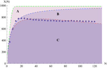
Figure 15: Scalability zones. Unnormalized throughput data $X(N)$ from Fig. 1 overlaid on scalability zones denoted $A,B$ and $C$ consistent with Table 1

Figure 15 presents a case in point. At low load, the WebSphere data lies in Zone A which is bounded by concurrent linearity on the upper side and synchronous contention on the lower side. The data is closer to the lower bound for $N<20$. The new interpretation of these data is that synchronous queueing appears to dominate scalability at low loads. At $N=20$, just like ice melting, the behavior of WebSphere changes rather dramatically as it starts to transition across Zone B and onto the upper side of Zone C. Above $N\geq 40$, WebSphere oscillates along the boundary between Zones C and B.

We know from our extended MRM model that Zone C means load-dependent service is superimposed on top of synchronous messaging in Zone B. This could be occurring for many reasons. Some examples are: priority sorting of the message queue, garbage collection or undesirable memory leaks. We cannot provide a definite explanation without a more thorough investigation of the architecture but that is the job of the software architect or the software engineer, not the performance analyst.

However, we can help the software architect or engineer by directing their attention to the $\mathcal{O}(N^{2})$ performance degradation in the USL model and explaining that Zone C involves synchronous requests with exchange-dependent service. In this way, the zones interpretation can quickly narrow the range of potential causes; something that would otherwise be very difficult to do. As implausible as this may seem to the casual reader, it is our experience that hints of this type are more than sufficient to trigger “Eureka!” moments among those most knowledgeable about the architectural details.

Another practical insight, that emerges from our Zones view, is also worth noting. The zones in Fig. 15 suggest one way to improve throughput performance, viz., attempt to replace the synchronous messaging, evident in Zones B and C, with asynchronous messaging. This strategy is analogous to the well-known performance gains that can be achieved by replacing synchronous (blocking) I/O with asynchronous (non-blocking) I/O. See wiki/Asynchronous_I/O.

Clearly, asynchronous messaging should make throughput scale almost linearly (Gustafson’s dream of Sects. 2.3 and 4.4) but only for very low loads. Beyond $N\simeq 10$ users, the throughput reaches saturation and (8) tells us that user response-time will begin to climb up the proverbial “hockey stick” handle. However, such linearity may not be desirable from a performance management perspective. It may be preferable to reach saturation more slowly and accommodate more aggregate users. Since this is tantamount to keeping on the upper side of Zone B, it is only necessary to ensure that the prepping repairman effect be minimized in the application. It is not necessary to eliminate synchronous messaging.

6 CONCLUSION

In this paper, we have used event-based simulation as an exploratory tool to accomplish several things. Simulation has confirmed the USL parametric modeling equation as being physical in the sense that it corresponds to the synchronous bound on throughput in a particular queueing model: a prepping machine repairman (Sect. 4.5). This result is the generalization of an earlier theorem concerning a queueing interpretation of Amdahl’s law based on rational functions [Gun 02].

By virtue of our approach, we have shown that Amdahl and Gustafson scaling laws are also unified by the same queueing model, viz., the machine-repairman model. Moreover, corollary 1 is a lower bound on throughput; synchronous throughput, and therefore represents worst-case scalability. With this physical interpretation, it follows immediately that Amdahl’s law can be “defeated” more conveniently than proposed in [Nel 96] by simply requiring that all requests be issued asynchronously.

To understand the USL in terms of the machine repairman, the standard queueing model had to be extended to include: (i) synchronous queueing (Sect. 3.3) and (ii) state-dependent service (Sects. 3.2. The precise nature of the synchronous queueing was only revealed by simulation, because the analytic equations used in the proof of theorem 2 are steady-state equations. Consequently, they hide the details of how the synchronization occurs, as well as obscuring how it controls the possible statistical distributions of the $S$ and $Z$ times in Table 2.

The simulation models provide a more intuitive understanding of how all these effects combine in a non-mathematical way. They also reveal how “real world” applications might behave (Table 1) and how this behavior is reflected in the parametric models used for statistical regression (Table 1). It is this concrete physical interpretation of the USL regression parameters that make it a more practical tool than the traditional queueing-model approach for assessing application scalability.

Finally, our investigations have led us to abandon the usual goal of fitting any particular nonlinear scalability model to data. Rather, we treat the data as dynamic and thus capable of making transitions between scalability zones (Sect. 5) as a function of load. Each of these zones comes with a well-defined interpretation in terms of queueing effects and this can be vital for system architects and performance engineers when considering how to get into a better scalability zone.

7 ACKNOWLEDGMENTS

One of us (NJG) thanks Guerrilla-graduates Denny Chen and Paul Puglia for helpful remarks that inspired the proofs of theorems 1 and 2.

TRADEMARKS

JavaOne is a service mark of Sun Microsystems, Inc. Mathematica is a registered trademark of Wolfram Research, Inc. SIMUL8 is a registered trademark of SIMUL8 Corporation. WebSphere is a registered trademark of IBM Corporation. All other Trademarks, product and company names are the property of their respective owners.

References

- AMBC [90] M. Ajmone-Marsan, G. Balbo, and G. Conte. Performance Models of Multiprocessor Systems. MIT Press, Boston, Mass., 1990.
- Amd [67] G. Amdahl. Validity of the single processor approach to achieving large scale computing capabilities. Proc. AFIPS Conf., 30:483–485, Apr. 18-20 1967.
- Bro [95] F. P. Brooks. The Mythical Man-Month. Addison-Wesley, Reading, MA, anniversary edition, 1995.
- GH [98] D. Gross and C. Harris. Fundamentals of Queueing Theory. Wiley, 1998.
- Gun [93] N. J. Gunther. “A simple capacity model for massively parallel transaction systems”. In Proc. CMG Conf., pages 1035–1044, San Diego, California, December 1993.
- Gun [96] N. J. Gunther. Understanding the MP effect: Multiprocessing in pictures. In Proc. CMG Conf., pages 957–968, San Diego, CA, Dec 1996.
- Gun [02] N. J. Gunther. A new interpretation of Amdahl’s law and Geometric scalability. arxiv.org/abs/cs/0210017, Oct 2002.
- Gun [05] N. J. Gunther. Analyzing Computer System Performance Using Perl::PDQ. Springer-Verlag, Heidelberg, Germany, 2005.
- Gun [07] N. J. Gunther. Guerrilla Capacity Planning. Springer-Verlag, Heidelberg, Germany, 2007.
- Gun [08] N. J. Gunther. A general theory of computational scalability based on rational functions. arxiv.org/abs/0808.1431, Aug 2008.
- Gus [88] J. L. Gustafson. “Reevaluating Amdahl’s law”. Comm. ACM, 31(5):532–533, 1988.
- [12] J. Holtman. The use of “R” for system performance analysis. In Proc. CMG Conf., pages 791–802, Las Vegas, Nevada, Dec 2004.
- [13] J. Holtman. Using a discrete simulation tool for modeling. In Proc. CMG Conf., pages 161–172, Las Vegas, Nevada, Dec 2004.
- KH [92] L. Kleinrock and J-H. Huang. On parallel processing systems: Amdahl’s law generalized and some results on optimal design. IEEE Trans. Software Eng., 18(5):434–447, 1992.
- Nel [96] R. D. Nelson. Including queueing effects in Amdahl’s law. Comm. ACM, 39(12es):231–238, 1996.
- Pre [95] F. P. Preparata. Should Amdahl’s law be repealed? In ISAAC ’95: Proceedings of the 6th International Symposium on Algorithms and Computation, page 311, London, UK, Dec 4-6 1995. Springer-Verlag.
- RF [87] D. A. Reed and R. M. Fujimoto. Multicomputer Networks: Message Based Parallel Processing. MIT Press, Boston, Mass., 1987.
- Sch [67] A. L. Scherr. An Analysis of Time-Shared Computer Systems. MIT, Cambridge MA, 1967.
- Sut [08] H. Sutter. Break Amdahl’s law! www.ddj.com/hpc-high-performance-computing/205900309, Jan 2008.
- ZSEG [82] J. Zahorjan, K. C. Sevcik, D. L. Eager, and B. Galler. Balanced job bound analysis of queueing networks. Comm. ACM, 25(2):134–141, Feb 1982.