Steady state of Stochastic Sandpile Models

Abstract

We study the steady state of the abelian sandpile models with stochastic toppling rules. The particle addition operators commute with each other, but in general these operators need not be diagonalizable. We use their abelian algebra to determine their eigenvalues, and the Jordan block structure. These are then used to determine the probability of different configurations in the steady state. We illustrate this procedure by explicitly determining the numerically exact steady state for a one dimensional example, for systems of size $\leq 12$, and also study the density profile in the steady state.

1 Introduction

Sandpile models with stochastic toppling rules are important subclass of sandpile models deepak . The first such model was studied by Manna manna , and these are usually known as Manna models in the literature. They are able to describe the avalanche behavior seen experimentally in the piles of granular media much better than the deterministic models rice . Also, in numerical studies, one gets better scaling collapse, and consequently, more reliable estimates for the values of the critical exponents, than for models with deterministic toppling rules chessa ; campelo .

Unfortunately, at present, the theoretical understanding of models with stochastic toppling rules is much less than that of their deterministic counterparts, e.g. the Bak-Tang -Wiesenfeld (BTW) model btw . For example, there is no analogue of the burning test to distinguish the transient and the recurrent states of a general Manna model. For the deterministic case, it is known that all the recurrent configurations occur with equal probability in the steady state. A similar characterization of the steady state is not known in the Manna case. The steady state has been explicitly determined only for the fully directed stochastic models asap ; rittenberg . In some cases, one can formally characterize the recurrent states of the model, e.g. the $1$-dimensional Oslo rice pile model, but a straightforward direct depth-first calculation of the exact probabilities of different configurations in the steady state takes $\mathcal{O}(exp{(L^{3})})$ steps where $L$ is the system length oslo . While the exact values of the critical exponents have been conjectured for $(1+1)$ dimensional directed Manna model kloster ; paczuski , the prototypical undirected Manna model in one dimension has resisted an exact solution so far dickman1 ; dickman2 ; dickman3 . In higher dimensions, most of the studies are only numerical, and deal with the estimation of the critical exponents of avalanche distribution, and the universality class of the model chessa ; pietronero ; biham ; lubeck ; menech ; mohanty1 ; bonachela ; mohanty2 .

While the original Manna model did not have the abelian property of the BTW model, one can construct stochastic toppling rules with abelian property sasm . In this paper, we discuss this abelian version of the stochastic Manna model. It is a special case of the more general Abelian Distributed Processors Model (ADP) deepak . We shall use the terms Deterministic Abelian Sandpile Models (DASM) and Stochastic Abelian Sandpile Models (SASM), if we need to distinguish between these two classes of models.

We use the algebra of the addition operators to determine the steady state of the model. This algebraic approach provides a computationally efficient method to determine the Markov evolution matrix of the model. The addition operators of SASM are not necessarily diagonalizable even if we restrict ourselves to the space of recurrent configurations. Using the abelian algebra we determine a generalized eigenvector basis in which the operators reduce to Jordan block form. We also define a transformation matrix between this basis and the configuration basis, and express the steady state in the latter basis. This procedure is illustrated by explicitly writing out the case of a one dimensional Manna model. In this special case, we can show that each Jordan block is at most of dimension $2$. We determine the numerically exact steady state of the model for systems of size up to $12$ and determine the asymptotic density profile by extrapolating the results.

This paper is organized as follows: In section $2$, we define the model precisely. In section $3$, we define the addition operators for the model, and discuss their algebra. Calculation of the eigenvalues and the Jordan block structure of the addition operators are given in section $4$. The transformation matrix between the generalized eigenvector basis and the configuration basis is determined in section $5$ and is used to determine the steady state vector in the configuration basis in section $6$. The exact numerical determination of the steady state is discussed in section $7$ with some concluding remarks in section $8$.

2 The Model

We define a generalized Manna model on a graph of $N$ sites with a non-negative integer height variable $z_{i}$ defined at each site $i$. Let the threshold height at $i$ be $z_{i}^{c}$, and the site is unstable if $z_{i}\geq z_{i}^{c}$. If the system is stable, a sand grain is added at a randomly chosen site which increases the height by $1$. For each site $i$, there is a set of $\alpha_{i}^{max}$ lists $E_{\alpha,i}$ with $\alpha=1,2,\cdots,\alpha_{i}^{max}$. If a site is unstable, it relaxes by the following toppling rule: we decrease its height by $z_{i}^{c}$. Then, with probability $p_{\alpha,i}$, we select the list $E_{\alpha,i}$, independent of any previous selections, and then add one grain to each site in that list. If a site occurs more than once in the list, we add that many grains to that site.

Toppling at a site can make other sites unstable and they topple in their turn, until all the lattice sites are stable. It follows from the abelian property of the model that the probabilities of different final stable configurations are independent of the order in which different unstable sites are toppled.

We illustrate these rules with some examples below.

• Model A (The one dimensional Manna model): The graph is $L$ sites on a line and $z_{i}^{c}=2$, for all sites. On toppling each grain is transfered to its neighbors with equal probability. Hence we have $\alpha_{i}^{max}=3$, for all $i$, with $E_{1,i}=\{i-1,i-1\}$, $E_{2,i}=\{i-1,i+1\}$, and $E_{3,i}=\{i+1,i+1\}$ and $p_{1,i}=p_{3,i}=1/4$ and $p_{2,i}=1/2$. Also grains can move out of the system if toppling occurs at a boundary site.

• Model B (The one dimensional dissipative Manna model): Same as model A except that on toppling a grain can move out of the system with probability $\epsilon$. Then $\alpha_{i}^{max}=6$ and the lists of neighbors $E_{1}=\{i-1,i-1\}$, $E_{2}=\{i-1,i+1\}$, $E_{3}=\{i+1,i+1\}$, $E_{4}=\{i-1\}$, $E_{5}=\{i+1\}$ and $E_{6}=\Phi$, where $\Phi$ is an empty set. The corresponding probabilities are $p_{1,i}=p_{3,i}=(1-\epsilon)^{2}/4$, $p_{2,i}=(1-\epsilon)^{2}/2$, $p_{4,i}=p_{5,i}=\epsilon(1-\epsilon)/2$ and $p_{6,i}=\epsilon^{2}$.

  In this case, one can use periodic boundary conditions, as there is dissipation at all sites. the steady state is critical only in the limit $\epsilon\rightarrow 0$. For the models A and B, it is easy to see that all stable configurations occur in the steady state with non-zero probability. We can also define stochastic models where the recurrent configurations form only an exponentially small fraction of all stable configurations. An example of this type is

• Model C: The graph is a square lattice with $N$ sites and $z_{\mathbf{i}}^{c}=2$. Under toppling, with equal probability two particles are transfered to either horizontal or vertical neighbors. Hence $\alpha_{i}^{max}=2$ with $E_{1,\mathbf{i}}=\{\mathbf{i}+\mathbf{e}_{x},\mathbf{i}-\mathbf{e}_{x}\}$ and $E_{2,\mathbf{i}}=\{\mathbf{i}+\mathbf{e}_{y},\mathbf{i}-\mathbf{e}_{y}\}$ with $p_{1,\mathbf{i}}=p_{2,\mathbf{i}}=1/2$.

In the following we will mostly confine ourselves to Model A. The treatment of other cases presents no special difficulties.

3 The addition operators and their algebra

Let us denote the space of stable states as $\Gamma$ spanned by $\Omega=\displaystyle\prod_{i=1}^{N}z_{i}^{c}$ basis vectors labeled by $C$. We define $P(C,t)$ as the probability of finding the system in the basis $C$ at time $t$. To each set $\{P(C,t)\}$, we associate a vector $|P(t)\rangle$ belonging to the vector space $\Gamma$, and write

$$|P(t)\rangle=\sum_{C}P(C,t)|C\rangle.$$ (1)

We define the particle addition operators $\textbf{a}_{i}$ for all $i$ as linear operators acting on $\Gamma$ as follows: Consider adding a sand grain at site $i$ in a configuration $C$, and relaxing the system until a stable configuration is reached. For stochastic toppling rules, the resulting state is not necessarily a basis vector corresponding to a unique stable configuration, but a linear combination of them. If the resulting configuration is $C^{\prime}$ with probability $P_{i}(C^{\prime}|C)$, we define

$$\mathbf{a}_{i}|C\rangle=\sum_{C^{\prime}}P_{i}(C^{\prime}|C)|C^{\prime}\rangle,$$ (2)

for all $C$. Note that the action of any of these operators on a given configuration gives a unique probability state vector.

Eq. (2) is a formal definition of the operators $\{\mathbf{a}_{i}\}$. One can think of these as $\Omega\times\Omega$ matrices, but it is quite non-trivial to actually determine the matrix elements $P_{i}(C^{\prime}|C)$ explicitly from the toppling rules. This is because of the non-zero probability of an arbitrary large number of toppling before a steady state is reached.

For an example, consider the avalanches in model A for system of size $L=3$. Consider the $2^{3}$ stable configurations as the basis vectors and denote them by their height values $|z_{1},z_{2},z_{3}\rangle$. The action of $\textbf{a}_{2}$ on $|0,1,0\rangle$ will generate a unstable state $|0,2,0\rangle$. Using the toppling rules we can write the following set of equations for three unstable states

$$|0,2,0\rangle = \frac{1}{4}|2,0,0\rangle+\frac{1}{2}|1,0,1\rangle+\frac{1}{4}|0,0,2\rangle,$$

$$|2,0,0\rangle = \frac{1}{4}|0,2,0\rangle+\frac{1}{2}|0,1,0\rangle+\frac{1}{4}|0,0,0\rangle,$$

$$|0,0,2\rangle = \frac{1}{4}|0,2,0\rangle+\frac{1}{2}|0,1,0\rangle+\frac{1}{4}|0,0,0\rangle.$$ (3)

We see that there is a nonzero probability that the avalanche can continue for more than $s$ toppling, for any finite $s$. e.g. in the sequence $|0,2,0\rangle\rightarrow|2,0,0\rangle\rightarrow|0,2,0\rangle\cdots$. Thus straight forward application of the relaxation rules do not result in a finite procedure to determine the unstable vector $|0,2,0\rangle$ in terms of the stable configurations. Instead, we have to write Eq. (3) as a matrix equation

$$\textbf{M}\begin{bmatrix}|0,2,0\rangle\\ |2,0,0\rangle\\ |0,0,2\rangle\end{bmatrix}=\begin{bmatrix}|1,0,1\rangle\\ |0,1,0\rangle\\ |0,0,0\rangle\end{bmatrix},$$ (4)

and then invert it. More generally, the determination of $P(C^{\prime}|C)$ involves working in a large space of unstable configurations.

For example in model A, there are $2^{L}$ stable configurations, where each site has $0$ or $1$ particle. Total number of particles is at most $L$. On adding one particle, the number of particles can become $L+1$, where initially, only one site will have height $2$. However, it is easy to verify that by toppling one can generate configurations where the number of particles at a site is much greater than $2$. In fact, all the $L+1$ particles could be at the same site. Then the total number of stable and unstable configurations $\Omega^{\prime}$ is the number of ways one can distribute $L+1$ particles on $L$ sites . It is easily seen that $\Omega^{\prime}$ varies as $4^{L}$, and one needs to invert a matrix of size $\mathcal{O}(\Omega^{\prime}\times\Omega^{\prime})$.

In this paper we will use the operator algebra to obtain an efficient method to determine the probabilities $P(C^{\prime}|C)$ explicitly which requires inverting a matrix only of size $2^{L}\times 2^{L}$. It has been shown sasm that the addition operators for different sites commute i.e.

$$[\mathbf{a}_{i},\mathbf{a}_{j}]=0\rm{,~{}~{}~{}for~{}all~{}}i,j.$$ (5)

Unlike the DASM, the inverse operators $\{\mathbf{a}^{-1}_{i}\}$ for SASM need not exist, even if we restrict ourselves to the set of recurrent configurations. This is because among the recurrent states, one can have two different initial probability vectors that yield the same resultant vector. This makes the determination of the matrix form of the operators difficult for this model.

Apart from the abelian property, the operators also satisfy a set of algebraic equations. For simplicity of presentation, now on we consider $z_{i}^{c}=z_{c}$ and $p_{\alpha,i}=p_{\alpha}$ for all sites. Then consecutive addition of $z_{c}$ grains at a site ensures that the site will topple once and transfers $z_{c}$ grains to its neighbors, irrespective of the initial height. Then the operators obey the following equation

$$\mathbf{a}_{i}^{z_{c}}=\sum_{\alpha}p_{\alpha}\mathbf{a}^{E_{\alpha,i}}\rm{~{}for~{}}1\leq i\leq N,$$ (6)

where we have used the notation $\mathbf{a}^{E}=\displaystyle\prod_{x\epsilon E}\mathbf{a}_{x}$ for any list $E$, and

$$\mathbf{a}_{i}=\mathbf{1},$$ (7)

for sites $i$ outside the lattice. In particular for the examples in Section $2$, these equations are as follows

$$\mathbf{a}_{i}^{2} = \frac{1}{4}(\mathbf{a}_{i-1}+\mathbf{a}_{i+1})^{2}\rm{~{}~{}~{}~{}~{}~{}~{}~{}~{}~{}~{}~{}~{}~{}~{}~{}~{}~{}~{}~{}~{}~{}~{}for~{}Model~{}A,}$$ (8)

$$\mathbf{a}_{i}^{2} = [\frac{1-\epsilon}{2}\mathbf{a}_{i-1}+\frac{1-\epsilon}{2}\mathbf{a}_{i+1}+\epsilon\mathbf{1}]^{2}\rm{~{}~{}~{}~{}~{}for~{}Model~{}B,~{}and~{}}$$ (9)

$$\mathbf{a}_{\mathbf{i}}^{2} = \frac{1}{2}(\mathbf{a}_{\mathbf{i}-\mathbf{e}_{x}}\mathbf{a}_{\mathbf{i}+\mathbf{e}_{x}}+\mathbf{a}_{\mathbf{i}-\mathbf{e}_{y}}\mathbf{a}_{\mathbf{i}+\mathbf{e}_{y}})\rm{~{}~{}~{}~{}~{}~{}~{}~{}for~{}Model~{}C.}$$ (10)

4 Jordan Block structure of the addition operators

In general the matrices $\{\mathbf{a}_{i}\}$ need not be diagonalizable. However, using the abelian property, we can construct a common set of generalized eigenvectors for all the operators $\{a_{i}\}$ such that in this basis the matrices simultaneously reduce to Jordan block form. These generalized eigenvectors split the vector space $\Gamma$ into disjoint subspaces, each corresponding to distinct set of eigenvalues. There will be at least one common eigenvector in each subspace, for all the addition operators.

Proof: Consider one of the operators, say $\mathbf{a}_{1}$. Let $\Gamma_{1}$ be the subspace of $\Gamma$ spanned by the (right) generalized eigen vectors of $\mathbf{a}_{1}$ corresponding to the eigenvalue $a_{1}$. There is at least one such generalized eigenvector, so $\Gamma_{1}$ is non-null. We pick one of the other addition operators, say $\mathbf{a}_{2}$. From the fact that $\mathbf{a}_{2}$ commutes with $\mathbf{a}_{1}$, it immediately follows that $\mathbf{a}_{2}$ acting on any vector in the subspace $\Gamma_{1}$ leaves it within the same subspace. Diagonalizing $\mathbf{a}_{2}$ within this subspace, we construct a possibly smaller but still non-null subspace $\Gamma_{2}$ which is spanned by simultaneous eigenvectors of $\mathbf{a}_{1}$ and $\mathbf{a}_{2}$ with eigenvalues $a_{1}$ and $a_{2}$. Repeating this argument with the other operators, one can construct vectors which are simultaneous eigenvectors of all the $\{\mathbf{a}_{i}\}$.

Let $|\psi\rangle$ be such an eigenvector, with

$$\mathbf{a}_{i}|\psi\rangle=a_{i}|\psi\rangle\rm{,~{}~{}~{}for~{}}\rm{~{}}\rm{~{}}1\leq i\leq N.$$ (11)

Then from Eq.($6$)the eigenvalues satisfy the following set of equations

$$a_{i}^{z_{c}}=\sum_{\alpha}p_{\alpha}a^{E_{\alpha,i}}\rm{~{}~{}~{}for~{}}\rm{~{}}\rm{~{}}1\leq i\leq N,$$ (12)

where we have used the notation $a^{E}=\displaystyle\prod_{x\epsilon E}a_{x}$, for any list $E$.

Rather than work with this general case, we will consider the special case in model A for simplicity. No extra complications occur in the more general case. Then, from Eq.(8), the corresponding eigenvalue equation is

$$a_{i}^{2}=\frac{1}{4}(a_{i-1}+a_{i+1})^{2}\rm{,~{}~{}~{}for~{}}\rm{~{}}\rm{~{}}1\leq i\leq L$$ (13)

These are L coupled quadratic equations in $L$ complex variables $\{a_{i}\}$. We can reduce them to $L$ linear equations by taking square root

$$\eta_{i}a_{i}=\frac{1}{2}(a_{i-1}+a_{i+1}),$$ (14)

where $\eta_{i}=\pm 1$. The Eq. (7) sets the values for the eigenvalues of $\mathbf{a}_{0}$ and $\mathbf{a}_{L+1}$ which are

$$a_{1}=a_{L+1}=1.$$ (15)

There are $2^{L}$ different choices for the set of $L$ different $\eta$’s and for each such choice, we get a set of eigenvalues $\{a_{i}\}$. In general, there will be degenerate sets of eigenvalues and the degeneracy arises if one of the $a_{i}$ is zero. Using the triangular inequality it is easy to show that

$$2|a_{i}|\leq|a_{i-1}|+|a_{i+1}|,$$ (16)

i.e. $|a_{i}|$ are convex functions of discrete variables $i$. Then, given the boundary condition in Eq. (15), there could at most be one $a_{i}=0$ in the solution for a given $\{\eta_{i}\}$, which means that each eigenvalue set can be at most doubly degenerate.

Finding the number of degeneracies of solutions is interesting but difficult in general. We show that for $L=3$ (mod $4$) the number of such degenerate sets of eigenvalues $\geq 2^{(L+1)/2}$.

Proof: Consider the system of length $L=4m+3$, with $m$ being a non negative integer. For any given set $\{\eta_{i}\}$, $i=1$ to $2m+2$, it is possible to construct a solution $\{b_{i}\}$ of Eq. (14) with $i\leq 2m+2$ which satisfies $b_{0}=1$ and $b_{2m+2}=0$. Clearly, from Eq.(14), if we have the solution $\{a_{i}\}$ corresponding to a particular set $\{\eta_{j}\}$, one can construct the solution $\{a_{i}^{\prime}\}$ corresponding to $\{\eta_{j}^{\prime}=-\eta_{j}\}$ using $a_{j}^{\prime}=(-1)^{j}a_{j}$. Using this symmetry we extend $\{b_{i}\}$ ($i=1$ to $(L+1)/2$) to form a set $\{a_{i}\}$ for $i=1$ to $L$ as follows:

$$a_{i} = b_{i}\rm{~{}~{}~{}~{}~{}~{}~{}~{}~{}~{}~{}~{}~{}~{}~{}~{}~{}for~{}}i\leq 2m+2,$$ (17)

$$= (-1)^{i}b_{L+1-i}\rm{~{}~{}~{}for~{}}i>2m+2.$$ (18)

This is a solution of Eq.(14) for the set $\{\eta^{\prime}_{i}\}$ with

$$\eta_{i}^{\prime} = \eta_{i}\rm{~{}~{}~{}~{}~{}~{}~{}~{}~{}~{}~{}~{}~{}~{}~{}~{}~{}for~{}}i\leq 2m+2,$$ (19)

$$= -\eta_{L+1-i}\rm{~{}~{}~{}~{}~{}~{}~{}~{}for~{}}i>2m+2.$$ (20)

and this solution $\{a_{i}\}$ satisfies the boundary conditions $a_{0}=1$, $a_{L+1}=1$, and $a_{2m+2}=0$ (Fig.$1$). There are $2^{2m+2}$ such solutions possible corresponding to all possible sets of $\{\eta_{i}^{\prime}\}$, and this gives the lower bound for the number of degenerate solutions.

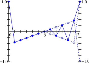
Figure 1: Schematic of a solution of Eq.(14) for $L=11$ with $a_{6}=0$, and $a_{0}=a_{12}=1$. The filled circles represent the values of the solution $\{a_{i}\}$.

A direct numerical calculation for $L\leq 20$ shows that if $L\neq 3$ (mod $4$), all $2^{L}$ sets of eigenvalues are distinct. We present the degeneracies of the solutions in Table.$1$. Calculation for simple choices of $\eta$ shows that the degeneracies are possible only if $L=3$ (mod $4$).

For example, consider $\eta_{i}=-1$ for $i=L$ and for the rest of the sites it is $1$. Then $a_{i}$ is of the form $a_{i}=1-\alpha i$, for all $i$. If we want this to be zero for $i=k$, we must have $\alpha=1/k$. Then, requiring that the equation (14) be satisfied at $i=L$, gives $3L=4k+1$, i.e. $L=3$ (mod $4$). Similarly for the set with $\eta_{L-1}=-1$ and $1$ for rest of the sites imposes a condition on length $3L=8k+1$, which is also a subset of $L=3$ (mod $4$). Finding a general proof that degeneracies occur only if $L=3$ (mod $4$) remain an open problem.

For each degenerate subspace there is a generalized eigenvector linearly independent of the eigenvector corresponding to the eigenvalue of the subspace. In general, let us denote them by $|\{a_{i}\};n\rangle$, where $n=1$ for the eigenvector and $n=2$ for the generalized eigenvector. For non-degenerate subspace $n$ can only be $1$. The vectors satisfy the following equations

$$\mathbf{a}_{i}|\{a_{j}\};1\rangle = a_{i}|\{a_{j}\};1\rangle,$$

$$\mathbf{a}_{i}|\{a_{j}\};2\rangle = a_{i}|\{a_{j}\};2\rangle+\alpha_{i}|\{a_{j}\};1\rangle,$$ (21)

where $\alpha$’s are complex numbers. Then using the Eq. (14) it can be shown easily that $\alpha$’s satisfy the following equation

$$\eta_{i}\alpha_{i}=\frac{1}{2}(\alpha_{i-1}+\alpha_{i+1}).$$ (22)

This is similar to the Eq. (14), except the boundary conditions which are

$$\alpha_{0}=\alpha_{L+1}=0.$$ (23)

For a given set of $\{\eta_{i}\}$, these are $L$ simultaneous set of homogeneous linear equations which has infinitely many possible solutions. In order to get a single solution we choose $\alpha_{i}=1$ if $a_{i}=0$, without loss of generality. This corresponds to choosing a particular normalization of the rank $2$ eigenvectors. The solution of both the equations (14) and (22) can be easily obtained numerically. The generalized eigenvectors and the Jordan block form of the addition operators for the system of size $L=3$ are given in the appendix.

L	$g$	$N_{1}$	$N_{2}$	$N_{3}$	$N_{4}$	$N_{5}$	$N_{6}$	$N_{7}$	$N_{8}$	$N_{9}$	$N_{10}$
3	4	0	4
7	40	0	0	8	24
11	136	0	0	0	8	0	120
15	1304	0	0	0	4	32	48	288	560
19	3024	0	0	0	0	0	8	0	288	0	2432

Table 1: Degeneracies arise if one of the $a_{i}$ is zero in a solution of Eq.(14). In the table, $g$ denotes the total number of solutions with one of the $a_{i}=0$ i.e. the total number of degenerate sets of solution. $N_{i}$ is the number of solutions with the eigenvalue $a_{i}=0$. Values for the other half of the system can be obtained using symmetry.

5 Matrix representation in the configuration basis

Given the well defined action of the addition operators on the generalized eigenvectors it is possible to define a transformation matrix $\mathbf{M}$ between the configuration basis and the generalized eigenvector basis.

$$|\{z_{i}\}\rangle=\sum_{j}\mathbf{M}_{\{z_{i}\},j}|\psi_{j}\rangle,$$ (24)

where $|\{z_{i}\}\rangle$ is the basis vector of $\Gamma$ corresponding to the height configuration $\{z_{i}\}$ and $|\psi_{j}\rangle$ is the $j$th generalized eigenvector. Let us express the configuration $|\{0\}\rangle$, with all sites empty, as a linear combination of all the generalized eigenvectors.

$$|\{0\}\rangle=\sum_{j}c_{j}|\psi_{j}\rangle,$$ (25)

where $c_{j}$s are constants. Then all the stable configurations can be obtained by adding grains at properly chosen sites in $|\{0\}\rangle$.

$$|\{z_{i}\}\rangle=\prod_{i}\mathbf{a}_{i}^{z_{i}}|\{0\}\rangle=\sum_{j}c_{j}\prod_{i}\mathbf{a}_{i}^{z_{i}}|\psi_{j}\rangle,$$ (26)

and hence

$$\mathbf{M}_{\{z_{i}\},j}=\langle\{z_{i}\}|\prod_{i}\mathbf{a}_{i}^{z_{i}}|\psi_{j}\rangle.$$ (27)

The action of the addition operators on the generalized eigenvectors, for example Eq.(21) for model A, would generate the elements of the matrix $\mathbf{M}$. Given $\mathbf{M}$, we can get the eigenvectors of $\mathbf{a}_{i}$, in the configuration basis, in particular, the steady state vector, by the inverse transformation

$$|\psi_{j}\rangle=\mathbf{M}^{-1}|\{z_{i}\}\rangle.$$ (28)

The addition operators in the configuration basis are obtained using the similarity transformation $\mathbf{M}\mathbf{a}^{J}_{i}\mathbf{M}^{-1}$. An explicit form of $\mathbf{M}$ for model A of length $L=3$ is given in the appendix.

6 Determination of the steady state vector

The time-evolution of the system is Markovian and the evolution operator $\mathbf{W}$ is defined by the master equation

$$|P(t+1)\rangle=\mathbf{W}|P(t)\rangle,$$ (29)

where $|P(t)\rangle$ and $|P(t+1)\rangle$ are the state of the system at time $t$ and $t+1$, respectively. We can write the time-evolution operator in terms of the addition operators as

$$\mathbf{W}=\frac{1}{L}\sum_{i}\mathbf{a}_{i}.$$ (30)

Then the common eigenvector of all the addition operators corresponding to eigenvalue $1$ is the steady state vector of the system. The steady state vector can be determined in the stable configuration basis using the matrix $\mathbf{M}^{-1}$. For model A of length $L=3$ the steady state vector is

$$|S\rangle= \frac{13}{392}|0,0,0\rangle+\frac{1}{16}|1,0,0\rangle+\frac{47}{392}|0,1,0\rangle+\frac{3}{16}|1,1,0\rangle$$ (31)

$$+\frac{1}{16}|0,0,1\rangle+\frac{13}{98}|1,0,1\rangle+\frac{3}{16}|0,1,1\rangle+\frac{3}{14}|1,1,1\rangle,$$

where the stable configurations are denoted by $|z_{1},z_{2},z_{3}\rangle$ with $z_{i}$ as the height of the $i$th site. The amplitude of each term in the expansion are the probability of finding the steady state in the corresponding height configuration.

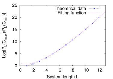
Figure 2: The ratio of the probability of the most probable configuration $C_{max}$ (all occupied) and the least probable configuration $C_{min}$ (all sites empty) plotted as a function of the system length $L$. The fitting function $f(x)=a-bL+cL\log L$, with $a=1.50,b=0.80$ and $c=0.94$.

7 Numerical Results

Here we numerically calculate the exact steady state of model A for different system length and discuss its properties. As shown in Eq. (14) and Eq. (22) the eigenvalues $\{a_{i}\}$ and the off-diagonal matrix elements $\{\alpha_{i}\}$ form sets of linear equations for a given set of $\{\eta_{i}\}$. We solve them by LU decomposition method. Because of the tridiagonal structure of the equations, only $\mathcal{O}(2^{L})$ number of steps are required to get the solution. The maximum number of steps ($\mathcal{O}(2^{3L})$) are required for the inversion of the transformation matrix $\mathbf{M}$. We have used the Gauss-Jordan elimination method for the inversion. It is important to note that, the maximum system length $L$, possible to treat by this method, is determined by the limited memory size of the computers, and not by the computation time. Using desktop computers we were able to determine $\mathbf{M}$ exactly for systems of size $L\leq 12$.

We note that as $L$ is increased, the second largest eigenvalue of $\mathbf{W}$ tends to $1/2$. Thus, the gap between the largest and the next largest eigenvalue of the relaxation matrix does not tend to zero. This gap measures the relaxation time of the system in terms of the macro-time unit of interval between addition of grains. However, the average duration of an avalanche measured in terms of micro-time unit of duration of a single toppling event does diverge, as system size increases.

An interesting question is the extent of variation between probabilities of different configurations in the steady state. In the one-dimensional Oslo model, for a system of $L$ sites, the ratio of probabilities of the most probable to the least probable configuration varies as $\exp(L^{3})$oslo . However in model A, we find that the ratio is not quit as large, and it only varies approximately as $\exp(0.94L\log L)$ (Fig.2) for large $L$.

This suggests that possibly the exact steady state has a product measure. To check this we define a product basis $|\psi^{\prime}\rangle=\displaystyle\prod_{i}|\psi_{i}^{\prime}\rangle$, where $|\psi_{i}^{\prime}\rangle$ could be any one of the two orthogonal vectors

$$|1^{\prime}\rangle = \cos\phi_{i}|1\rangle+\sin\phi_{i}|0\rangle,$$

$$|0^{\prime}\rangle = \sin\phi_{i}|1\rangle-\cos\phi_{i}|0\rangle,$$ (32)

with $\phi_{i}$ a real number. Then in this basis the steady state can be written as

$$|S\rangle=\sum_{\psi^{\prime}}P(\psi^{\prime})|\psi^{\prime}\rangle.$$ (33)

We choose $\{\phi_{i}\}$ so that the ratio between the amplitudes of basis vectors with next-largest and largest amplitudes becomes as small as possible (this would become zero, if the state was a product measure state). In Fig.3, we have plotted for system of size $L=12$, the relative amplitudes in both configuration basis and the optimized product basis as a function of the rank of the basis vectors with the vectors arranged in decreasing orders of their amplitudes. In the optimized basis the second highest probability is only $10$ times smaller than the highest probability. This implies that the steady state measure is not a product measure.

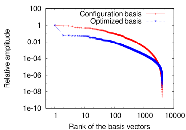
Figure 3: The amplitudes, normalized with its largest value, corresponding to the basis vectors in the steady state plotted as a function of the rank of the basis vectors. The vectors are arranged in decreasing orders of their amplitudes. The plot is given for the configuration basis and the optimized basis for model A of size $L=12$.

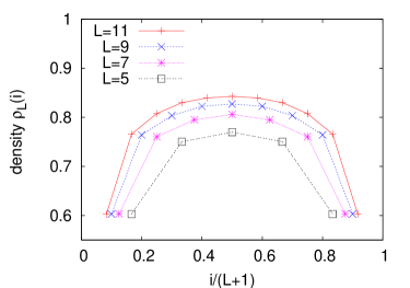
Figure 4: Average steady state density $\rho_{L}(i)$ at site $i$ for model A of different length $L$.

$~{}~{}~{}~{}~{}L~{}~{}~{}~{}~{}$	$~{}~{}~{}~{}~{}~{}\bar{\rho}_{L}~{}~{}~{}~{}~{}~{}$	$~{}~{}~{}~{}~{}~{}\rho_{L}(x_{m})~{}~{}~{}~{}~{}~{}$
2	0.583333	0.583333
3	0.634354	0.709184
4	0.669262	0.737000
5	0.695210	0.769704
6	0.715472	0.786491
7	0.731879	0.805897
8	0.745514	0.816009
9	0.757080	0.827217
10	0.767051	0.834600
11	0.775760	0.842665
12	0.783451	0.848054

Table 2: The values of particle density in the steady state for the model A of different length $L$. Here $\bar{\rho}_{L}$ denotes the steady state particle density averaged over all sites and $\rho_{L}(x_{m})$ denotes the steady state particle density at the central site.

L	$1/\bar{\rho}_{\infty}$	$B$	$\nu_{\perp}$
3	1.061	1.128	0.656
4	1.049	1.132	0.641
5	1.053	1.132	0.646
6	1.049	1.131	0.640
7	1.050	1.131	0.641
8	1.049	1.130	0.639
9	1.049	1.130	0.639
10	1.049	1.130	0.639
11	1.049	1.130	0.639

Table 3: The sequential fit of the functional form in Eq. (35) to the data for average particle density for model A of different length $L$ given in Table $2$.

The steady state density for different sites are plotted in Fig. 4 for different system sizes. Amongst the different fitting forms that we tried, the following functional form gives the best fit

$$\frac{1}{\rho_{L}(x)}=\frac{1}{\bar{\rho}_{\infty}}+b[\frac{1}{(x+d)^{\nu_{\perp}}}+\frac{1}{(L+1-x+d)^{\nu_{\perp}}}],$$ (34)

where $\bar{\rho}_{\infty},b,\nu_{\perp}$ and $d$ are real numbers. Using this functional form the steady state particle density averaged over all sites for system of size $L$ can be written as

$$\frac{1}{\bar{\rho}_{L}}=\frac{1}{\bar{\rho}_{\infty}}+\frac{B}{(L+\delta)^{\nu_{\perp}}},$$ (35)

where $B$ is a real number and $\bar{\rho}_{\infty}$ is the asymptotic value of the average particle density. The exact value of $\bar{\rho}_{L}$ and the particle density at the central site $\rho_{L}(x_{m})$ are listed in the Table $2$ for different system sizes. The sequential fitting method is used to find the values of $\bar{\rho}_{\infty}$, $B$, $\nu_{\perp}$ and $\delta$ from these data. For a given choice of $\delta$, these values are obtained numerically by solving the Eq. (35) for three consecutive lengths $L-1$, $L$ and $L+1$. Best convergence of the values of $\bar{\rho}_{\infty}$, $B$ and $\nu_{\perp}$ are obtained for $\delta=1.1$, which are tabulated in Table $3$. The asymptotic value of the average particle density converges to $\bar{\rho}_{\infty}=0.953$ which is close to the more precise estimate $0.94885(7)$, from Monte Carlo simulations dickman1 .

8 Concluding remarks.

For a general SASM with $N$ sites, the calculation of eigenvalues involves solving $N$ coupled polynomial equations in $N$ variables. This can be done in polynomial time in $\Omega$, the number of stable configurations of the model. These are then used to construct the transformation matrix ${\bf M}$ of size $\Omega\times\Omega$. Finally inverting the matrix ${\bf M}$ gives us the eigenvectors of the evolution operator, in particular the steady state.

Of course, to determine the steady state of any Markov chain on $\Omega$ states, we need to determine the eigenvectors of the evolution matrix of size $\Omega\times\Omega$. The point here is that the specification of the toppling rules does not directly specify the evolution matrix, and determining the matrix elements of the latter from the toppling rules is computationally very nontrivial. Using the abelian property, we are able to tackle this problem.

For a generic model with some parameters, e.g. the model B, except for special symmetries, one does not expect degeneracies in eigenvalues to occur for a generic value of the parameters. For special values of the parameters, if there is a non-trivial Jordan block structure of the evolution operator, it would show up in the time-dependent correlation functions of the model by the presence of terms of the type $t\exp(-\lambda_{j}t)$, in addition to the usual sum of terms of the type $\exp(-\lambda_{j}t)$.

In particular we have explicitly calculated the steady state for a specific model (model A in section 2) of length L$\leq 12$. Extrapolating the results we determined the asymptotic density profile in the steady state. The power-law profile of deviations from the mean value near the ends would be important for determining the avalanche exponents of the model lubeck2 . This remains an interesting open problem.

Appendix A Appendix

Here we give some details of the explicit calculation of the steady state, and the matrix representation of addition operators for model A of length $L=3$.

The eight sets of eigenvalues obtained by solving Eq.(14) are $(1,1,1)$, $(-1,1,-1)$, $(\frac{1}{3},-\frac{1}{3},\frac{1}{3})$, $(-\frac{1}{3},-\frac{1}{3},-\frac{1}{3})$, $(\frac{1}{2},0,-\frac{1}{2})$, and $(-\frac{1}{2},0,\frac{1}{2})$ with the last two sets repeated twice.

For writing the matrix structure of the addition operators, we choose the order of the eigenvectors same as the order of the eigenvalues mentioned above. For the degenerate subspace we order the eigenvector $|\{a_{i}\};1\rangle$, defined in Eq.(21), before the generalized eigenvector $|\{a_{i}\};2\rangle$. Then in this basis the matrices corresponding to the addition operators have the following Jordan block form.

$$\textbf{a}^{J}_{1}=\begin{pmatrix}1~{}&~{}0~{}&~{}0~{}&~{}0~{}&~{}0~{}&~{}0~{}&~{}0~{}&~{}0\\ 0~{}&-1&~{}0~{}&~{}0~{}&~{}0~{}&~{}0~{}&~{}0~{}&~{}0\\ 0~{}&~{}0~{}&~{}\frac{1}{3}~{}&~{}0~{}&~{}0~{}&~{}0~{}&~{}0~{}&~{}0\\ 0~{}&~{}0~{}&~{}0~{}&-\frac{1}{3}&~{}0~{}&~{}0~{}&~{}0~{}&~{}0\\ 0~{}&~{}0~{}&~{}0~{}&~{}0~{}&~{}\frac{1}{2}~{}&~{}\frac{1}{2}~{}&~{}0~{}&~{}0\\ 0~{}&~{}0~{}&~{}0~{}&~{}0~{}&~{}0~{}&~{}\frac{1}{2}~{}&~{}0~{}&~{}0\\ 0~{}&~{}0~{}&~{}0~{}&~{}0~{}&~{}0~{}&~{}0~{}&-\frac{1}{2}&-\frac{1}{2}\\ 0~{}&~{}0~{}&~{}0~{}&~{}0~{}&~{}0~{}&~{}0~{}&~{}0~{}&-\frac{1}{2}\end{pmatrix},$$ (36)

$$\textbf{a}^{J}_{2}=\begin{pmatrix}1~{}&~{}0~{}&~{}0~{}&~{}0~{}&~{}0~{}&~{}0~{}&~{}0~{}&~{}0\\ 0~{}&~{}1~{}&~{}0~{}&~{}0~{}&~{}0~{}&~{}0~{}&~{}0~{}&~{}0\\ 0~{}&~{}0~{}&-\frac{1}{3}&~{}0~{}&~{}0~{}&~{}0~{}&~{}0~{}&~{}0\\ 0~{}&~{}0~{}&~{}0~{}&-\frac{1}{3}&~{}0~{}&~{}0~{}&~{}0~{}&~{}0\\ 0~{}&~{}0~{}&~{}0~{}&~{}0~{}&~{}0~{}&~{}1~{}&~{}0~{}&~{}0\\ 0~{}&~{}0~{}&~{}0~{}&~{}0~{}&~{}0~{}&~{}0~{}&~{}0~{}&~{}0\\ 0~{}&~{}0~{}&~{}0~{}&~{}0~{}&~{}0~{}&~{}0~{}&~{}0~{}&~{}1\\ 0~{}&~{}0~{}&~{}0~{}&~{}0~{}&~{}0~{}&~{}0~{}&~{}0~{}&~{}0\end{pmatrix},$$ (37)

$$\textbf{a}^{J}_{3}=\begin{pmatrix}1~{}&~{}0~{}&~{}0~{}&~{}0~{}&~{}0~{}&~{}0~{}&~{}0~{}&~{}0\\ 0~{}&-1&~{}0~{}&~{}0~{}&~{}0~{}&~{}0~{}&~{}0~{}&~{}0\\ 0~{}&~{}0~{}&~{}\frac{1}{3}~{}&~{}0~{}&~{}0~{}&~{}0~{}&~{}0~{}&~{}0\\ 0~{}&~{}0~{}&~{}0~{}&-\frac{1}{3}&~{}0~{}&~{}0~{}&~{}0~{}&~{}0\\ 0~{}&~{}0~{}&~{}0~{}&~{}0~{}&-\frac{1}{2}&-\frac{1}{2}&~{}0~{}&~{}0\\ 0~{}&~{}0~{}&~{}0~{}&~{}0~{}&~{}0~{}&-\frac{1}{2}&~{}0~{}&~{}0\\ 0~{}&~{}0~{}&~{}0~{}&~{}0~{}&~{}0~{}&~{}0~{}&~{}\frac{1}{2}~{}&~{}\frac{1}{2}\\ 0~{}&~{}0~{}&~{}0~{}&~{}0~{}&~{}0~{}&~{}0~{}&~{}0~{}&~{}\frac{1}{2}\end{pmatrix},$$ (38)

The transformation matrix $\mathbf{M}$, discussed in section $5$, between the generalized eigenvector basis and the configuration basis has the following form

$$\textbf{M}=\begin{pmatrix}1~{}&~{}1~{}&~{}1~{}&~{}1~{}&~{}1~{}&~{}1~{}&~{}1~{}&~{}1\\ 1~{}&-1~{}&~{}1/3~{}&-1/3~{}&~{}1~{}&~{}1/2~{}&-1~{}&-1/2\\ 1~{}&~{}1~{}&-1/3~{}&-1/3~{}&~{}1~{}&~{}0~{}&~{}1~{}&~{}0\\ 1~{}&-1~{}&-1/9~{}&~{}1/9~{}&~{}1/2~{}&~{}0~{}&-1/2~{}&~{}0\\ 1~{}&-1~{}&~{}1/3~{}&-1/3~{}&-1~{}&-1/2~{}&~{}1~{}&~{}1/2\\ 1~{}&~{}1~{}&~{}1/9~{}&~{}1/9~{}&-3/4~{}&-1/4~{}&-3/4~{}&-1/4\\ 1~{}&-1~{}&-1/9~{}&~{}1/9~{}&-1/2~{}&~{}0~{}&~{}1/2~{}&~{}0\\ 1~{}&~{}1~{}&-1/27~{}&-1/27~{}&-1/4~{}&~{}0~{}&-1/4~{}&~{}0\end{pmatrix},$$ (39)

where the configuration basis vectors are chosen in the following order $(0,0,0)$, $(1,0,0)$, $(0,1,0)$, $(1,1,0)$, $(0,0,1)$, $(1,0,1)$, $(0,1,1)$, and $(1,1,1)$. The matrix is non-singular, and the inverse can be calculated numerically. Using the similarity transformation $\mathbf{M}\mathbf{a}_{1}^{J}\mathbf{M}^{-1}$ we find matrix representation of the addition operator $\mathbf{a}_{1}$ in the configuration basis.

$$\textbf{a}_{1}=\begin{pmatrix}0~{}&~{}\frac{2}{7}~{}&~{}0~{}&~{}\frac{4}{49}~{}&~{}0~{}&~{}0~{}&~{}0~{}&~{}0\\ 1~{}&~{}0~{}&~{}0~{}&~{}0~{}&~{}0~{}&~{}\frac{1}{24}~{}&~{}0~{}&~{}\frac{1}{9}\\ 0~{}&~{}\frac{4}{7}~{}&~{}0~{}&~{}\frac{22}{49}~{}&~{}0~{}&~{}0~{}&~{}0~{}&~{}0\\ 0~{}&~{}0~{}&~{}1~{}&~{}0~{}&~{}0~{}&~{}\frac{1}{12}~{}&~{}0~{}&~{}\frac{19}{72}\\ 0~{}&~{}0~{}&~{}0~{}&~{}0~{}&~{}0~{}&~{}\frac{7}{24}~{}&~{}0~{}&~{}\frac{1}{9}\\ 0~{}&~{}\frac{1}{7}~{}&~{}0~{}&~{}\frac{16}{49}~{}&~{}1~{}&~{}0~{}&~{}0~{}&~{}0\\ 0~{}&~{}0~{}&~{}0~{}&~{}0~{}&~{}0~{}&~{}\frac{7}{12}~{}&~{}0~{}&~{}\frac{37}{72}\\ 0~{}&~{}0~{}&~{}0~{}&~{}\frac{1}{7}~{}&~{}0~{}&~{}0~{}&~{}1~{}&~{}0\end{pmatrix},$$ (40)

The other operators can also be determined similarly.

References

- (1) Dhar D.: Theoretical studies of self-organized criticality. Physica A 369, 29 (2006)
- (2) Manna S. S.: Two-state model of self-organized criticality. J. Phys. A: Math. Gen. 24, L363 (1991)
- (3) Frette V., Christensen K., Mathe-Sorensen A., Feder J., Jossang T. and Meakin P.: Avalanche dynamics in a pile of rice. Nature 379, 49 (1996)
- (4) Chessa A., Stanley H. E., Vespignani A., and Zapperi S.: Universality in sandpiles. Phys. Rev E. 59, R12 (1999)
- (5) Dickman R., and Campelo J. M. M.: Avalanche exponents and corrections to scaling for a stochastic sandpile. Phys. Rev. E 67, 066111 (2003)
- (6) Bak P., Tang C., and Wiesenfeld K.: Self-organized criticality: An explanation of the 1/f noise. Phys. Rev. Lett. 59, 381 (1987); Self-organized criticality. Phys. Rev. A 38, 364 (1988)
- (7) Povolotsky A. M., Priezzhev V. B., and Hu C. K.: The asymmetric avalanche process. J. Stat Phys 3, 1149 (2003)
- (8) Alcaraz F. C., and Rittenberg V.: Directed abelian algebras and their applications to stochastic models. arXiv:0806.1303
- (9) Dhar D.: Steady state and relaxation spectrum of the Oslo rice-pile model. Physica A 340, 535 (2004)
- (10) Kloster M., Maslov S., Tang C.: Exact solution of a stochastic directed sandpile model. Phys. Rev. E 63, 026111 (2001)
- (11) Paczuski M., Bassler K. E.: Theoretical results for sandpile models of self-organized criticality with multiple topplings. Phys. Rev. E 62, 5347 (2000)
- (12) Dickman R., Alva M., Muoz, Peltola J., Vespignani A., Zapperi S.: Critical behavior of a one-dimensional fixed-energy stochastic sandpile. Phys. Rev. E 64, 056104 (2001)
- (13) Stilck J. F., Dickman R. and Vidigal R. R.: Series expansion for a stochastic sandpile. J. Phys. A: Math. Gen. 37, 1145 (2004)
- (14) Vidigal R. R. and Dickman R.: Asymptotic behavior of the order parameter in a stochastic sandpile. J. Stat. Phys. 118, 1 (2005)
- (15) Pietronero L., Vespignani A., and Zapperi S.: Renormalization scheme for self-organized criticality in sandpile models. Phys. Rev. Lett. 72, 1690 (1994); Vespignani A., Zapperi S., and Pietronero L.: Phys. Rev. E 57, 1711 (1995)
- (16) Ben-Hur A., and Biham O.: Universality in sandpile models. Phys. Rev. E 53, R1317 (1996); Milshtein E., Biham O., and Solomon S.: Universality classes in isotropic, Abelian, and non-Abelian sandpile models. Phys. Rev. E 58, 303 (1998)
- (17) Lubeck S.: Moment analysis of the probability distribution of different sandpile models. Phys. Rev. E 61, 204 (2000)
- (18) Menech M. D.: Comment on “Universality in sandpiles”. Phys. Rev. E 70, 028101 (2004)
- (19) Mohanty P. K. and Dhar D.: Generic sandpiles have directed percolation exponents, Phys. Rev. Lett. 89, 104303 (2002)
- (20) Bonachela J. A. Ramasco J. J. Chate H., Dornic I. and Munoz M. A., Sticky grains do not change the universality class of isotropic sandpiles, Phys. Rev. E 74, 050102 (2006)
- (21) Mohanty P. K. and Dhar D.: Critical behavior of sandpile models with sticky grains, Physica A 384, 34 (2007)
- (22) Dhar D.: Some results and a conjecture for Manna’s stochastic sandpile model. Physica A 270, 69 (1999)
- (23) Lubeck S. and Dhar D.: Continuously varying exponents in sandpile models. J. Stat. Phys. 102, 1 (2001)