Quantifying the cost of simultaneous non-parametric approximation of several samples

Abstract

We consider the standard non-parametric regression model with Gaussian errors but where the data consist of different samples. The question to be answered is whether the samples can be adequately represented by the same regression function. To do this we define for each sample a universal, honest and non-asymptotic confidence region for the regression function. Any subset of the samples can be represented by the same function if and only if the intersection of the corresponding confidence regions is non-empty. If the empirical supports of the samples are disjoint then the intersection of the confidence regions is always non–empty and a negative answer can only be obtained by placing shape or quantitative smoothness conditions on the joint approximation. Alternatively a simplest joint approximation function can be calculated which gives a measure of the cost of the joint approximation, for example, the number of extra peaks required.

, , t1Research supported in part by Sonderforschungsbereich 475, Technical University of Dortmund

1 Introduction

We consider the following problem in non-parametric regression. Given $k$ samples

$${\mbox{\boldmath$y$}_{in_{i}}}=\{(t_{ij},y_{ij}):j=1,\ldots,n_{i}\},\,i=1,\ldots,k,$$ (1)

with supports

$$S_{in_{i}}=\{t_{i1}<t_{i2}<\ldots<t_{in_{i}}\},\,i=1,\ldots,k,$$ (2)

the question to be answered is whether they can be simultaneously represented by a common function $f.$ The standard approach is to assume that the data sets were generated according to the model

$$Y_{in_{i}}(t)=f_{i}(t)+\sigma_{i}Z_{i}(t),\,\,i=1,\ldots,k,\quad t\,\in\,[0,\,1],$$ (3)

and then to consider the null and alternative hypotheses

$$H_{0}:f_{1}=\ldots=f_{k}\quad H_{1}:f_{i}\neq f_{j}\quad\text{for some }i,j.$$ (4)

We assume that the noise processes $Z_{i}(t),i=1,\ldots,k$ are independent and standard Gaussian white noise. Individual samples generated under (3) will be denoted by

$${\mbox{\boldmath$Y$}_{in_{i}}}=\{(t_{ij},Y_{ij}):j=1,\ldots,n_{i}\},\,i=1,\ldots,k.$$

Here and in the following we use minuscule letters to denote general data sets and majuscule letters for data generated under (3). We shall mostly restrict attention to the case $k=2;$ the extension to more samples poses no problems.

Within this setup it is possible to construct tests which are asymptotically consistent if $\lim n_{i}=\infty,\,i=1,2$, and which can detect alternatives converging to the null hypothesis at certain rates. This may be formalized by putting

$$f_{1}(t)-f_{2}(t)=f_{1,n_{1}}(t)-f_{2,n_{2}}(t)=\Delta_{n}(t),\quad n=\min(n_{1},n_{2})$$ (5)

where $\Delta_{n}$ is a difference function and measures the rate of convergence to the null hypothesis. The best result seems to be that of Neumeyer and Dette, (2003) who construct a test which can detect alternatives which converge to the null hypothesis at the optimal rate $\Delta_{n}=\text{O}(n^{-1/2}).$ If the supports are equal, $S_{in_{i}}=\{t_{1},\ldots,t_{n_{i}}\},\,i=1,2,$ then it is not difficult to construct such a test as the differences $Y_{1n_{1}}(t_{j})-Y_{2n_{2}}(t_{j})$ do not depend on $f$ (see for example Delgado, (1992) and Fan and Lin, (1998)). The result of Neumeyer and Dette, (2003) continues to hold even if the supports are disjoint, $S_{1n_{1}}\cap S_{2n_{2}}=\emptyset.$ In this case, however, there are difficulties which can be most clearly seen in the case of exact data

$$y_{ij}=f_{i}(t_{ij}),\,\,t_{ij}\in S_{in_{i}},\quad i=1,2.$$

If we denote the supremum norm on $[0,\,1]$ by $\|\cdot\|_{\infty}$ then the null and alternative hypotheses of (4) may be rewritten as

$$H_{0}:\|f_{1}-f_{2}\|_{\infty}=0,\quad H_{1}:\|f_{1}-f_{2}\|_{\infty}>0.$$ (6)

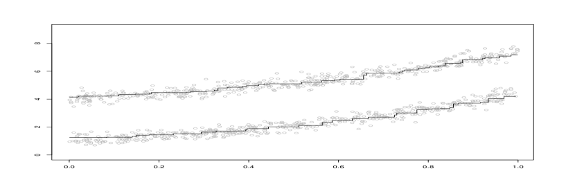
Figure 1: The top panel shows two samples each of size 500 generated by $Y_{1}(t)=\exp(1.5t)+0.25Z(t)$ and $Y_{2}(t)=\exp(1.5t)+3+0.25Z(t)$ together with the approximating monotonic curves. The design points were taken to be i.i.d. random variables uniformly distributed on $[0,\,1].$ The centre panel shows a joint approximating function with 514 local extreme values. The bottom panel shows a sample of size $n=1000$ generated using the function of the centre panel.

If the values of $f_{1}$ and $f_{2}$ are known only on disjoint sets $S_{1n_{1}}$ and $S_{2n_{2}}$ respectively, then it is not possible to decide between $H_{0}$ and $H_{1}$. This continues to hold even if $f_{1}$ and $f_{2}$ are subject to qualitative smoothness conditions such as infinite differentiability: all one does is to interpolate the data points using such a function. The addition of noise and the use of asymptotics does not solve the problem as indicated by Figure 1. The top panel shows two data sets of sizes $n_{1}=n_{2}=500$ generated according to $Y_{1}(t)=\exp(1.5t)+0.25Z_{1}(t)$ and $Y_{2}(t)=\exp(1.5t)+3+0.25Z_{2}(t)$ with disjoint supports taken to be i.i.d. uniform random variables on $[0,1].$ The centre panel shows a joint piecewise constant approximating function with 514 local extreme values. It can be made infinitely differentiable by convolving it with a Gaussian kernel with a small bandwidth. The bottom panel shows a sample of size $n=1000$ generated using the function of the centre panel. It looks very much like the two original data sets.

In order to distinguish between $H_{0}$ and $H_{1}$ it is necessary to place either quantitative conditions on $f_{1}$ and $f_{2}$ such as $\|f_{1}^{(1)}\|_{\infty}\leq 1,\,\|f_{2}^{(1)}\|_{\infty}\leq 1,$ or shape restrictions such as $f_{1}$ and $f_{2}$ being monotone. In spite of this all conditions imposed in the literature are of a qualitative form: Hall and Hart, (1990), a bounded first derivative; Härdle and Marron, (1990), Hölder continuity; King et al., (1990), ‘at least uniform continuity´; Kulasekera, (1995), Kulasekera and Wang, (1997), a continuous second derivative; Munk and Dette, (1998), Hölder continuity of order $\beta>1/2$; Dette and Neumeyer, (2001), a continuous $r$th derivative: Lavergne, (2001), a second derivative which is uniformly Lipschitz of order $\beta,\,0\leq\beta\,<1$; Neumeyer and Dette, (2003), continuous derivatives of order $d\geq 2$. The problem is one of uniform convergence which is required to make the results applicable for finite $n$ and which does not follow from qualitative conditions alone. What can be said is that if the functions differ, then any joint approximation will become more complicated as the sample sizes increase. It is this increase in complexity which we call the cost of the simultaneous approximation. This is shown in Figure 1 where the individual approximations are monotone (top panel) but the simplest joint approximation has 514 local extreme values (centre panel). In the remainder of the paper we show how the quantification can be carried out. Our approach can be split into two parts:

• Firstly, for each sample ${\mbox{\boldmath$y$}_{in_{i}}}$ we define a so called approximation region ${\mathcal{A}}_{in_{i}}$ which specifies those functions $f_{i}$ for which the model (3) is an adequate approximation for the sample. The intersection of the approximation regions ${\mathcal{A}}_{1,n_{1}}\cap{\mathcal{A}}_{2,n_{2}}$ contains all those functions which simultaneously approximate both samples. It is also the approximation region for the simultaneous approximation. A similar idea in the context of the one-way table in the analysis of variance is expounded in Davies, (2004).

• Secondly, using some measure of complexity we regularize within each approximation region by choosing the simplest function which is consistent with the data. This is in the spirit of Donoho, (1988) who pointed out that in non-parametric regression and density problems it is possible only to give lower bounds on certain quantities of interest such the number of modal values.

In Section 2 we define the approximation or confidence regions ${\mathcal{A}}_{in_{i}}$ and in Section 3 we apply the ideas and concepts to the problem of comparing regression functions.

2 Approximation regions

2.1 Single samples

The following is based on Davies et al., 2008c . We consider a single sample of data ${\mbox{\boldmath$Y$}}_{n}=(t_{i},Y(t_{i}))_{1}^{n}$ generated under the model

$$Y(t)=f(t)+\sigma Z(t)$$ (7)

where we take the $t_{i}$ to be ordered. Based on this model we consider two different approximation or confidence regions ${\mathcal{A}}_{n}$ and ${\mathcal{A}}_{n}^{*}$ defined as follows. For any function $g$ and any interval $I\subset[0,\,1]$ we put

$$w(g,{\mbox{\boldmath$Y$}}_{n},I)=\frac{1}{\sqrt{|I|}}\,\sum_{t_{i}\in I}(Y(t_{i})-g(t_{i}))$$ (8)

where $|I|$ denotes the number of points $t_{i}\in I.$ The confidence region ${\mathcal{A}}_{n}$ is defined by

$${\mathcal{A}}_{n}({\mbox{\boldmath$Y$}}_{n},{\mathcal{I}}_{n},\sigma,\tau_{n})=\{g:\,\max_{I\in{\mathcal{I}}_{n}}\,|w({g,\mbox{\boldmath$Y$}}_{n},I)|\ \leq\sigma\sqrt{\tau_{n}\log(n)\,}\,\}.$$ (9)

where ${\mathcal{I}}_{n}$ is a collection of intervals of $[0,\,1]$. We restrict attention to the cases where ${\mathcal{I}}_{n}$ is either the set of all intervals or a set of intervals of the form

$${\mathcal{I}}_{n}(\lambda)=\left\{[t_{l(j,k)},\,t_{u(j,k)}]\,:\,l(j,k)=\lfloor(j-1)\lambda^{k}+1\rfloor,\right.$$ (10)

$$\left.u(j,k)=\min\{\lfloor j\lambda^{k}\rfloor,n\},j=1,\ldots,\lceil n\lambda^{-k}\rceil,k=1,\ldots,\lceil\log n/\log\lambda\rceil\right\}.$$

for some $\lambda>1.$ Our default choice is the (wavelet) dyadic scheme ${\mathcal{I}}_{n}(2)$. For any given $\alpha$ and collection of intervals ${\mathcal{I}}_{n}$ we define $\tau_{n}(\alpha)$ by

$${\mbox{\boldmath$P$}}\left(\max_{I\in{\mathcal{I}}_{n}}\frac{1}{\sqrt{|I|}}\Big{|}\sum_{i\in I}Z(t_{i})\Big{|}\leq\sqrt{\tau_{n}(\alpha)\log n\,}\right)=\alpha.$$ (11)

The value of $\tau_{n}(\alpha)$ may be determined by simulations. These show that for ${\mathcal{I}}_{n}={\mathcal{I}}_{n}(2)$ we have $\tau_{n}(0.95)\leq 3$ for all $n\geq 500.$ If ${\mathcal{I}}_{n}$ contains all singletons $\{t_{i}\}$, as will always be the case, it follows from Dümbgen and Spokoiny, (2001) and Kabluchko, (2007) that $\lim_{n\rightarrow\infty}\tau_{n}(\alpha)=2$ for any $\alpha.$ One immediate consequence of (11) is

$${\mbox{\boldmath$P$}}(f\in{\mathcal{A}}_{n}({\mbox{\boldmath$Y$}}_{n},{\mathcal{I}}_{n},\sigma,\tau_{n}(\alpha)))=\alpha$$ (12)

so that ${\mathcal{A}}_{n}$ is a universal, exact and non-asymptotic confidence region for $f$ of size $\alpha.$

The confidence region (9) treats all intervals equally. The second confidence region ${\mathcal{A}}_{n}^{*}$ downweights the importance of small intervals and is defined as follows. Dümbgen and Spokoiny, (2001) extended Lèvy’s uniform modulus of continuity of the Brownian motion and showed that

$$\sup_{0<s<t<1}\frac{\frac{(B(t)-B(s))^{2}}{t-s}-2\log(1/(t-s))}{\log(\log(e^{e}/(t-s)))}<\infty\quad\text{a.s.}$$ (13)

If we embed the partial sums $\sum_{i\in I}^{j}Z(t_{i})/\sqrt{|I|},\,I\in{\mathcal{I}}_{n},$ in a standard Brownian motion it follows that

$$\sup_{I\in{\mathcal{I}}_{n}}\frac{(\sum_{t_{j}\in I}Z(t_{j}))^{2}/|I|-2\log(n/|I|)}{\log(\log(e^{e}n/|I|)))}=\Gamma<\infty\quad\text{a.s.}.$$ (14)

This implies that for any $\alpha$ we can find a $\gamma_{n}=\gamma_{n}(\alpha)$ such that

$${\mathcal{A}}^{*}_{n}({\mbox{\boldmath$Y$}}_{n},{\mathcal{I}}_{n},\sigma,\gamma_{n}(\alpha))=\{g:\,|w({g,\mbox{\boldmath$Y$}}_{n},I)|$$

$$\leq \sigma\sqrt{2\log(n/|I|)+\gamma_{n}(\alpha)\log(\log(e^{e}n/|I|))}\,\,\text{for all}\,\,I\in{\mathcal{I}}_{n})\,\}.$$

is a universal, exact and non-asymptotic $\alpha$-confidence region for $f.$ The values of $\gamma_{n}$ may be determined by simulation. For $\alpha=0.95$ and with ${\mathcal{I}}_{n}={\mathcal{I}}_{n}(2)$ a good approximation for $\gamma_{n}(\alpha)$ for $n\geq 100$ is given by

$$\gamma_{n}(0.95)\approx 5.77-\exp(2.89-0.6\log(n)).$$ (16)

The confidence regions ${\mathcal{A}}_{n}({\mbox{\boldmath$Y$}}_{n},{\mathcal{I}}_{n},\sigma,\tau_{n})$ and ${\mathcal{A}}^{*}_{n}({\mbox{\boldmath$Y$}}_{n},{\mathcal{I}}_{n},\sigma,\gamma_{n})$ both require the true value of $\sigma.$ We indicate how this may be obtained from the data in such a manner that the confidence region now becomes honest (Li, (1989)) rather than exact. The following argument makes the somewhat casual remarks on the problem made in Davies et al., 2008c more precise. Using the normal approximation for the binomial $(n,1/2)$ distribution it follows that for an i.i.d. sample $(W_{1},\ldots,W_{n})$ with common continuous distribution $P$ with median $\text{med}(P)$

$${\mbox{\boldmath$P$}}\big{(}W_{(\lceil n/2+z_{\beta}\sqrt{n}/2\rceil)}\geq\text{med}(P)\big{)}=\beta$$

where $W_{(i)}$ denotes the $i$th order statistic of the sample and $z_{\beta}$ the $\beta$-quantile of the standard normal distribution. On putting $\beta=0.995$ we obtain

$${\mbox{\boldmath$P$}}\big{(}W_{(\lceil n/2+1.288\sqrt{n}\,\rceil)}\geq\text{med}(P)\big{)}=0.995.$$

We now apply this to the $\lfloor n/2\rfloor$ random variables

$$V_{i}=|Y_{2i-1}-Y_{2i}|,\quad i=1,\ldots,\lfloor n/2\rfloor.$$

It follows from Anderson, (1955) that whatever the value of the function $f$

$${\mbox{\boldmath$P$}}\big{(}V_{i}\geq 1.4826\sigma/\sqrt{2}\Big{)}\geq 1/2$$

and consequently

$${\mbox{\boldmath$P$}}\big{(}V_{(\lceil n/4+0.9108\sqrt{n}\,\rceil)}\geq 1.4826\sigma/\sqrt{2}\big{)}=0.995.$$

On using the corresponding result for the $\lfloor(n-1)/2\rfloor$ random variables

$$|Y_{2i}-Y_{2i+1}|,\quad i=1,\ldots,\lfloor(n-1)/2\rfloor$$

it follows that if we define ${\hat{\sigma}_{n}}$ to be the $\lceil n/2+1.814\sqrt{n}\,\rceil$ order statistic of the random variables

$$\frac{1.4826}{\sqrt{2}}|Y(t_{2})-Y(t_{1})|,\ldots,\frac{1.4826}{\sqrt{2}}|Y(t_{n})-Y(t_{n-1})|$$

then

$${\mbox{\boldmath$P$}}\big{(}{\hat{\sigma}_{n}}\geq\sigma\big{)}\geq 0.99$$

for all $n\geq 100$ say whatever the value of $f$. It follows that ${\mathcal{A}}_{n}({\mbox{\boldmath$Y$}}_{n},{\mathcal{I}}_{n},{\hat{\sigma}_{n}},\tau_{n})$ and ${\mathcal{A}}^{*}_{n}({\mbox{\boldmath$Y$}}_{n},{\mathcal{I}}_{n},{\hat{\sigma}_{n}},\gamma_{n})$ are now universal and non-asymptotic honest confidence regions whatever the value of $f$ but with $\alpha$ replaced by $\alpha-0.01,$

$${\mbox{\boldmath$P$}}\big{(}f\in{\mathcal{A}}_{n}({\mbox{\boldmath$Y$}}_{n},{\mathcal{I}}_{n},{\hat{\sigma}}_{n},\tau_{n}(\alpha))\big{)}\geq\alpha-0.01.$$ (17)

with the corresponding inequality for ${\mathcal{A}}_{n}^{*}.$ In spite of this the default value for ${\hat{\sigma}}_{n}$ we shall use in this paper is

$${\hat{\sigma}}_{n}=\frac{1.4826}{\sqrt{2}}\text{median}\,(|Y(t_{2})-Y(t_{1})|,\ldots,|Y(t_{n})-Y(t_{n-1})|).$$ (18)

It is simpler, the difference is in general small, it was used in Davies and Kovac, (2001), Davies et al., (2006), Davies et al., 2008a and it also corresponds to using the first order Haar wavelets to estimate $\sigma$ (Donoho et al., (1995)).

In Davies, (1995) implicit use is made of an confidence region based on the lengths of runs of the signs of the residuals. Explicit universal, honest and non-asymptotic confidence regions based on the signs of the residuals are to be found in Dümbgen, (1998, 2003, 2007) and Dümbgen and Johns, (2004).

2.2 A one-way table for regression functions

This section extends the approach given in Davies, (2004) for the one-way table to the case of regression functions. We consider $k$ samples ${\mbox{\boldmath$Y$}}_{in_{i}}=(t_{ij},Y_{i}(t_{ij}))_{j=1}^{n_{i}}$ generated under (3). As a first step we replace the $\alpha$ in (11) and (2.1) by $\alpha_{k}=\alpha^{1/k}$ where $k$ is the number of samples. This adjusts the size of each confidence region to take into account the number of samples. The confidence region for the $i$th sample is given by

$${\mathcal{A}}_{in_{i}}={\mathcal{A}}_{in_{i}}({\mbox{\boldmath$Y$}}_{in_{i}},{\mathcal{I}}_{in_{i}},{\hat{\sigma}}_{in_{i}},\tau_{in_{i}}(\alpha_{k}))=$$

$$\big{\{}g:\,\max_{I\in{\mathcal{I}}_{in_{i}}}\,|w({g,\mbox{\boldmath$Y$}}_{in_{i}},I)|\ \leq{\hat{\sigma}}_{in_{i}}\sqrt{\tau_{in_{i}}(\alpha_{k})\log(n_{i})\,}\,\,\big{\}}.$$

We denote by ${\mbox{\boldmath$P$}}_{\mbox{\boldmath$f$}}$ with ${\mbox{\boldmath$f$}}=(f_{1},\ldots,f_{k})$ the probability model where all the samples ${\mbox{\boldmath$Y$}}_{in_{i}},\,i=1,\ldots,k,$ are independently distributed and ${\mbox{\boldmath$Y$}}_{in_{i}}$ was generated under (3) with $f=f_{i},\,i=1,\ldots,k$. It follows from the choice $\alpha_{k}=\alpha^{1/k}$ that

$${\mbox{\boldmath$P$}}_{\mbox{\boldmath$f$}}\,(f_{i}\in{\mathcal{A}}_{in_{i}}({\mbox{\boldmath$Y$}}_{in_{i}},{\mathcal{I}}_{in_{i}},{\hat{\sigma}}_{in_{i}},\tau_{in_{i}}(\alpha_{k})),\,i=1,\ldots k)\geq\alpha\quad\text{for all}\quad{\mbox{\boldmath$f$}}.$$ (20)

All questions concerning the relationships between the functions $f_{i}$ can now be answered by using the confidence regions ${\mathcal{A}}_{in_{i}}$. For example, the question as to whether the $f_{i}$ are all equal translates into the question as to whether

$${\mathcal{A}}_{\mbox{\boldmath$n$}_{k}}=\cap_{i=1}^{k}{\mathcal{A}}_{in_{i}}=\cap_{i=1}^{k}{\mathcal{A}}_{in_{i}}({\mbox{\boldmath$Y$}}_{in_{i}},{\mathcal{I}}_{in_{i}},{\hat{\sigma}}_{in_{i}},\tau_{in_{i}}(\alpha_{k})),\quad{\mbox{\boldmath$n$}_{k}}=(n_{1},\ldots,n_{k})$$ (21)

is empty or not. If the supports $S_{in_{i}}$ of the samples are not disjoint then it is possible that the linear inequalities which define the confidence regions are inconsistent. In this case ${\mathcal{A}}_{\mbox{\boldmath$n$}_{k}}=\emptyset$ and there is no joint approximating function. If the supports $S_{in_{i}}$ of the samples are pairwise disjoint then ${\mathcal{A}}_{\mbox{\boldmath$n$}_{k}}$ is non–empty and so there always is a joint approximation function. Without further restrictions on the joint approximating function nothing more can be said. If however the joint approximating function is required to satisfy, for example, a shape constraint such as monotonicity, then it may be the case that there is no joint approximating function. Figure 1 shows just such a case where there are monotonic approximations for each sample individually but no monotonic joint approximation. To answer questions of this nature we must regularize within ${\mathcal{A}}_{\mbox{\boldmath$n$}_{k}}$ and this is the topic of the next section.

3 Regularization

3.1 Disjoint supports

We consider firstly the case when the supports $S_{in_{i}},i=1,\ldots,k$, are pairwise disjoint. In this case the joint approximation region ${\mathcal{A}}_{\mbox{\boldmath$n$}_{k}}$ is non-empty and will in general include many functions which would not be regarded as being acceptable. Indeed, it may be that ${\mathcal{A}}_{\mbox{\boldmath$n$}_{k}}$ does not contain any acceptable function. The definition of ‘acceptable’ will usually be formulated in terms of shape or quantitative smoothness constraints.

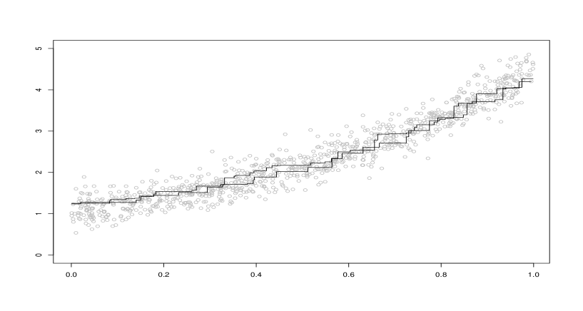
Figure 2: The upper panel shows the data of Figure 1 but with the values of $Y_{2}$ now given by $Y_{2}(t)=\exp(1.5t)+0.07+0.25Z(t).$ There is now a joint monotonic approximating function which is shown in the lower panel.

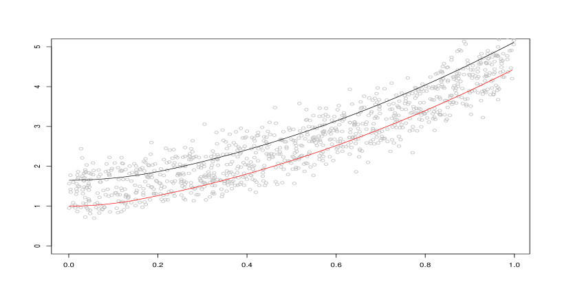
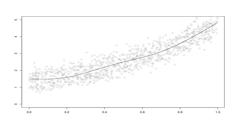
Figure 3: The upper panel shows the results of minimizing the total variation of the second derivative for the data of the upper panel of Figure 2 subject to monotonicity. The lower panel shows the corresponding result for the lower panel of Figure 2.

Alternatively, rather than impose prior restrictions, one can determine a simplest function in the joint approximating region. One possibility is to minimize the number of local extreme points of a function $g$ subject to $g\in{\mathcal{A}}_{{\mbox{\boldmath$n$}}_{k}}.$ Figure 1 shows an example of this approach where the joint approximating function has 514 internal local extreme points compared with monotone approximating functions for both data sets separately. The additional local extreme points can be regarded as the cost of the joint approximation. The same idea can be used if simplicity is defined in terms of smoothness, for example by minimizing the total variation $TV(g^{(2)})$ of the second derivative subject to $g$ lying in the approximation region. The upper panel of Figure 2 shows the data and curves of Figure 1 but with the values of the second sample reduced by an amount 2.3. There is now a joint monotone approximation which is shown in the lower panel of Figure 1 so there is no cost in terms of the number of local extreme values. If we minimize the total variation of the second derivative subject to the function being an adequate monotone approximation then there is a cost. The upper panel of Figure 3 shows the approximations of the two individual samples which minimize the total variation of the second derivatives subject to the functions being monotone. The lower panel of Figure 3 shows the joint approximation for the combined sample. The second derivatives are shown in Figure 4. The values of the total variation of the second derivative are are he values are 9.317 and 6.305 for the individual samples and 59.496 for the joint sample.

3.2 Intersecting supports

As mentioned in Section 1 the Neumeyer and Dette (2003) procedure can detect differences of the order of $n^{-1/2}.$ We now consider the size of detectable differences for our procedure in the case of equal supports. For simplicity we consider only the case $k=2$ and assume that the supports $S_{1n_{1}}$ and $S_{2n_{2}}$ are given by $t_{1i}=t_{2i}=i/n.$ We take ${\mathcal{I}}_{n}$ to be the set of all intervals but indicate below the adjustments required if ${\mathcal{I}}_{n}={\mathcal{I}}_{n}(\lambda)$ as in (10). We state the results using $\sigma_{1}$ and $\sigma_{2}$ rather than the estimates (18) and write $\tau_{n}=\tau_{n}(\alpha^{1/k}).$ If a joint approximating function ${\tilde{f}}_{n}$ exists then for any interval $I$ of $[0,\,1]$ we have

$$\frac{1}{\sqrt{|I|}}\left|\sum_{t_{i}\in I}(Y_{j}(t_{i})-f_{n}(t_{i}))\right|\leq\sigma_{i}\sqrt{\tau_{n}\log(n)}\,,\,\,j=1,\,2.$$

and hence

$$\frac{1}{\sqrt{|I|}}\left|\sum_{t_{i}\in I}(Y_{1}(t_{i})-Y_{2}(t_{i}))\right|\leq(\sigma_{1}+\sigma_{2})\sqrt{\tau_{n}\log(n)}\,\,.$$

For the noise we have with probability $\alpha$

$$\frac{1}{\sqrt{|I|}}\left|\sum_{t_{i}\in I}(Z_{1}(t_{i})-Z_{2}(t_{i}))\right|\leq(\sigma_{1}+\sigma_{2})\,\sqrt{\tau_{n}\log(n)}$$

and hence with probability $\alpha$

$$\frac{1}{\sqrt{|I|}}\left|\sum_{t_{i}\in I}(f_{1}(t_{i})-f_{2}(t_{i}))\right|\leq 2(\sigma_{1}+\sigma_{2})\sqrt{\tau_{n}\log(n)}\,\,.$$

Suppose now that $f_{1}$ and $f_{2}$ differ by an amount $\eta_{n}$ on an interval $I_{n}\subset[0,\,1]$, that is $f_{1}(t)-f_{2}(t)>\eta_{n},t\in I_{n}$ and that the length of $I_{n}$ is $\delta_{n}.$ As $I_{n}$ contains about $n\delta_{n}$ support points we see that

$$\frac{1}{\sqrt{n\delta_{n}}}n\delta_{n}\eta_{n}\leq 2(\sigma_{1}+\sigma_{2})\sqrt{\tau_{n}\log(n)}$$

which implies that no joint approximation will exist if

$$\sqrt{\delta_{n}}\,\eta_{n}>2(\sigma_{1}+\sigma_{2})\sqrt{\tau_{n}\log(n)/n}.$$ (22)

It follows that with probability of at least $\alpha$, deviations satisfying the latter inequality will be detected. If ${\mathcal{I}}_{n}={\mathcal{I}}_{n}(\lambda)$ as in (10) it follows that there exists an interval $I_{n}^{\prime}\subset I$ in ${\mathcal{I}}_{n}(\lambda)$ and of length $|I_{n}^{\prime}|\geq|I_{n}|/\lambda=\delta_{n}/\lambda$ for which $f_{1}(t)-f_{2}(t)>\eta_{n},\,t\in I_{n}^{\prime}.$ This requires replacing (22) by

$$\sqrt{\delta_{n}}\,\eta_{n}>2\sqrt{\lambda}(\sigma_{1}+\sigma_{2})\sqrt{\tau_{n}\log(n)/n}.$$ (23)

We consider a situation similar to that of Figure 1 as is shown in Figure 5. The sample sizes are $n=500$ with common supports $t_{j}=j/n$ and we take $\alpha$ to be 0.95 so that $\alpha_{k}=0.95^{1/2}=0.9747.$ For this choice of $\alpha$ and with ${\mathcal{I}}_{n}={\mathcal{I}}_{n}(2)$ simulations give $\tau_{n}=2.973.$ We set $f_{1}(t)=\exp(1.5t)$ and put $f_{2}(t)=f_{1}(t)$ except for $t\in[0.402,0.44]$ where $f_{2}(t)=f_{1}(t)+\eta_{n}.$ For this interval $\delta_{n}=20/500$ and so we expect to be able to detect deviations $\eta_{n}$ of the order

$$\eta_{n}=2\sqrt{2}(0.25+0.25)\sqrt{2.973\log 500\,}/\sqrt{20\,}=1.359$$ (24)

with probability of at least 0.95. For the data shown in Figure 5 the difference is detected with $\eta_{n}=0.575$ but not with $\eta_{n}=0.574.$

If we put $\delta_{n}=1$ in (22) so that the two functions deviate over the whole interval then

$$\eta_{n}>2\sqrt{2}(\sigma_{1}+\sigma_{2})\sqrt{\tau_{n}\log(n)/n\,}.$$ (25)

which implies that deviations of order $\sqrt{\log(n)/n\,}$ can be detected.

The same analysis can be carried through using the approximation region ${\mathcal{A}}_{n}^{*}.$ Corresponding to (22) we obtain

$$\eta_{n}h(\sqrt{\delta_{n}})\,>2(\sigma_{1}+\sigma_{2})/\sqrt{n}$$ (26)

where

$$h(\delta)=\frac{\delta}{2*\log(1/\delta)+\gamma_{n}(\alpha)\log\log(e^{e}/\delta)}\,,\,\,0<\delta\leq 1,$$ (27)

is monotonically increasing and $\gamma_{n}(\alpha)$ is bounded in $n$. In particular, if $\delta_{n}=1,$ then deviations of order $1/\sqrt{n}$ can be detected.

3.3 Adapting the taut string algorithm

The taut string algorithm of Davies and Kovac, (2001) has proved to be very effective in determining the number of local extremes of a function contaminated by noise (see Davies et al., 2008b ). We show how it may be adapted to the case of $k$ samples. Let $n\leq\sum_{i=1}^{k}n_{i}$ denote the number of different $t_{ij}$ values which we order as $0\leq t_{1}<\ldots<t_{n}\leq 1.$ For each sample we calculate the values of ${\hat{\sigma}_{in_{i}}}$ given by (18). We put

$$y_{m}=\frac{\sum_{t_{ij}=t_{m}}y_{ij}/{\hat{\sigma}_{in_{i}}}^{2}}{\sum_{t_{ij}=t_{m}}1/{\hat{\sigma}_{in_{i}}}^{2}}\,,\quad m=1,\ldots,n.$$ (28)

As a first step we check whether a joint approximating function exists. We do this by putting ${\tilde{f}}_{n}(t_{m})=y_{m}$ and then determining whether ${\tilde{f}}_{n}\in{\mathcal{A}}_{{\mbox{\boldmath$n$}}_{k}}$. If this is not the case we conclude that no joint approximation exists. If a joint approximation exists we put ${\hat{\Sigma}}_{m}=\sum_{t_{ij}=t_{m}}1/{\hat{\sigma}_{in_{i}}}^{2}$ and calculate the partial sums $y^{\circ}_{m}=\sum_{1}^{m}{\hat{\Sigma}}_{j}y_{j}$ and $A_{m}=\sum_{1}^{m}{\hat{\Sigma}}_{j}$ for $m=1,\ldots,\,n$ with $y^{\circ}_{0}=A_{0}=0$. The initial lower and upper bounds $L_{i}$ and $U_{i}$ are set to be $L_{i}=Y_{i}-D,\,U_{i}=Y_{i}+D$ where $D$ is chosen so large that the straight line joining $(0,0)$ and $(y^{\circ}_{n},A_{n})$ lies in the tube. For a given tube, the taut string through the tube and constrained to pass through $(0,0)$ and $(y^{\circ}_{n},A_{n})$ is calculated. The value of the estimate ${\tilde{f}}_{n}(t_{m})$ at the point $t_{m}$ is taken to be the left hand derivative of the taut string except for the first point where the right-hand derivative is taken. For each data set individually it is now checked whether ${\tilde{f}}_{n}\in{\mathcal{A}}_{in_{i}},i=1,\ldots,k.$ If this is the case the procedure ends. Otherwise those intervals for which the inequalities defining the ${\mathcal{A}}_{in_{i}}$ do not hold are noted and the tube is squeezed at all points $t_{j-1}$ and $t_{j}$ for which $t_{j}$ lies in such an interval. This is continued until a function ${\tilde{f}}_{n}\in{\mathcal{A}}_{{\mbox{\boldmath$n$}}_{k}}$ is found.

4 Comparison with other procedures

4.1 Analysis and simulations

As the approach developed in this paper is not comparable with others when the supports are disjoint, we restrict attention to the case of equal supports. For simplicity we take $k=2.$ For such data Delgado (1992) proposed the test statistic

$$T_{n}=\sqrt{n}\max_{1\leq j\leq n}|R(j)|/s_{n}^{*}=\max_{1\leq j\leq n}\left|\sum_{i=1}^{j}(Y_{1}(t_{i})-Y_{2}(t_{i}))\right|/(\sigma_{n}\sqrt{n})$$ (29)

where $\sigma_{n}$ is some quantifier of the noise. Under the null hypothesis $f_{1}=f_{2}=f$ the distribution of $T_{n}$ does not depend on $f$. In this special case the test statistic of Neumeyer and Dette also reduces to (29). If the data were generated under (3) then under $H_{0}$ the distribution of $T_{n}$ converges to that of $\max_{0\leq t\leq 1}|B(t)|$ where $B$ is a standard Brownian motion. The 0.95-quantile is approximately 2.24 which leads to rejection of $H_{0}$ if

$$T_{n}\geq 2.24.$$ (30)

Suppose now that the data are generated as in (3) with $f_{1}(t)=f_{2}(t)$ apart from $t$ in an interval $I$ of length $\delta_{n}$ where $f_{1}(t)-f_{2}(t)\geq\eta_{n}$. It follows from (30) that $H_{0}$ will be rejected with high probability if

$$\delta_{n}\eta_{n}\geq 4.48\sigma/\sqrt{n}$$ (31)

where $\sigma^{2}=\sigma_{1}^{2}+\sigma_{2}^{2}.$ If $\delta_{n}=1$ deviations of the order of $\sigma/\sqrt{n}$ can be picked up which contrasts with the $O(\sigma\sqrt{\log(n)/n})$ of (25). If however $\delta_{n}=1/\sqrt{n}$ it follows from (31) that the test statistic $T_{n}$ will pick up deviations of the order of $\sigma$. It follows from (22) and (26) that the methods based on ${\mathcal{A}}_{n}$ and ${\mathcal{A}}_{n}^{*}$ will both pick up deviations of the order of $\sigma\sqrt{\log(n)/\sqrt{n}\,}.$

Another test which is applicable in this situation is due to Fan and Lin (1998). If we denote the Fourier transform of the data sets by ${\tilde{Y}}_{1}(i)$ and ${\tilde{Y}}_{2}(i),i=1,\ldots,n,$ and order them as described in Fan and Lin (1998), their test statistic reduces to

$$T^{*}_{n}=\max_{1\leq m\leq n}\left|\frac{1}{\sqrt{m}}\sum_{i=1}^{m}(({\tilde{Y}}_{2}(i)-{\tilde{Y}}_{1}(i))^{2}/{\tilde{\sigma}}_{n}^{2}-1)\right|$$ (32)

where ${\tilde{\sigma}}_{n}$ is some estimate of the standard deviation of the ${\tilde{Y}}_{2}(i)-{\tilde{Y}}_{1}(i).$ For data generated under the model (3) the critical value of $T^{*}_{n}$ can be obtained by simulations. It is not as simple to determine the size of the deviations which can be detected by the test (32) as the test statistic is a function of the Fourier transforms and the differences in the functions must be translated into differences in the Fourier transforms. The first member of the sum in (32) is the difference of the means and this is given the largest weight. We do not pursue this further but give the results of a small simulation study.

We put $n=500$ and consider two samples of the form

$$Y_{1}(i/n) = Z_{1}(i/n),\quad i=1,\ldots,n=500$$ (33)

$$Y_{2}(i/n) = g(i/n)+Z_{2}(i/n),\quad i=1,\ldots,n=500$$ (34)

were generated where the $Z_{j}(i/n)$ are i.i.d $N(0,1)$ random variables with $g$ given by one of

(1) $$g_{1}(t)=\eta,\,0\leq t\leq 1,$$ (2) 

(3)  (4) 

(35)

where $U$ is uniformly distributed on $[0,3/4]$ and independent of the $Z_{i},i=1,2.$ The four procedures, Delgado–Neumeyer–Dette, Fan–Lin and those based on ${\mathcal{A}}_{n}$ and ${\mathcal{A}}_{n}^{*}$ were all calibrated to give tests of size $0.05$ for testing $g\equiv 0.$ The critical values for Delgado–Neumeyer–Dette and Fan–Lin tests are 2.22 and 6.97 respectively. The value of $\tau_{n}$ for the test based on ${\mathcal{A}}_{n}$ is 1.46 and the corresponding value of $\gamma_{n}$ for that based on ${\mathcal{A}}_{n}^{*}$ is 0.66. Figure 6 shows the power of the tests for different values of $\eta.$ The upper panels are the results for $g$ given by (35) (1) and (35) (2) and the lower panels for $g$ given by (35) (3) and (35) (4). The colour scheme is as follows: Delgado–Neumeyer–Dette blue, the Fan–Lin black, ${\mathcal{A}}_{n}$ green and ${\mathcal{A}}_{n}^{*}$ red. The results confirm the analysis given above. The Delgado–Neumeyer–Dette and Fan–Lin tests are better with $g$ given by (1) but if the mean difference is zero (2), or the interval is small (3) or both (4) then they are outperformed by the procedure based on ${\mathcal{A}}_{n}^{*}$ and, in case 4, also by that based on ${\mathcal{A}}_{n}.$

4.2 An application

We give an example with some real data from the area of thin-film physics. They give the number of photons of refracted X-rays as a function of the angle of refraction and were kindly supplied by Professor Dieter Mergel of the University of Duisburg-Essen. Two such data sets are shown in the top panel of Figure 7; the differences $y_{1}(t_{i})-y_{2}(t_{i})$ are shown in the bottom panel. Each data set is composed of 4806 measurements and the design points are the same. The samples differ in the manner in which the thin film was prepared. One of the questions to be answered is whether the results of the two methods are substantially different.

The noise levels for the data sets are the same, namely 8.317, which is explainable by the fact that the data are integer valued. The differences between the two data sets are concentrated on intervals each containing about 40 observations. The estimate (31) suggests that the differences will have to be of the order of 92 to be detected with a degree of certainty by the Delgado–Neumeyer–Dette test. The actual differences are of about this order and in fact the test fails to reject the null hypothesis at the 0.1 level. The realized value of the test statistic is 1.734 as against the critical value of 1.90 given in (30). The Fan-Lin test (32) rejects the null hypothesis at the 0.01 level. The realized value of the test statistic is 111.66 as against the critical value of 12.44 for a test of size $\alpha=0.01.$ Finally the tests based on ${\mathcal{A}}_{n}$ and ${\mathcal{A}}_{n}^{*}$ both reject the null hypothesis at the 0.01 level. The realized value of $\tau_{n}$ is 43.15 as against the critical value of 1.50. The realized value of $\gamma_{n}$ is 53.27 as against the critical value of 0.733.

Figure 4: The upper panel shows the second derivative iof the functions in the upper panel of Figure 3: the lower panel shows the corresponding result for the lower panel of Figure 3.

Figure 5: The upper panel shows the function $f_{1}(t)=\exp(1.5t)$ and the function $f_{2}$ which is equal to $f_{1}$ apart from the interval $[0.402,0.440]$ where $f_{2}(t)=f_{1}(t)+0.575$. The lower panel shows the two data sets $Y_{1}(t_{j})=f_{1}(t_{j})+0.25Z_{1}(t_{j})$ and $Y_{2}(t_{j})=f_{2}(t_{j})+0.25Z_{2}(t_{j})$ for $j=1,\ldots,500$ and with $t_{j}=j/500.$

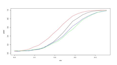
Figure 6: The top row shows the power functions of the four tests with $g$ given by (1) and (2). The bottom row shows the power functions of the four tests with $g$ given by (1) and (2). The Delgado–Neumeyer–Dette is shown in blue, the Fan–Lin test in black, the test based on ${\mathcal{A}}_{n}$ in green and that based on ${\mathcal{A}}_{n}^{*}$ in red.

Figure 7: The top and center panels show two data sets each of 4806 observations with the same design points. The lower panel shows the differences of the two samples.

References

- Anderson, (1955) Anderson, T. W. (1955). The integral of a symmetric unimodal function over a symmetric convex set and some probability inequalities. Proceedings of the American Mathematical Society, 6(2):170–176.
- Davies, (1995) Davies, P. L. (1995). Data features. Statistica Neerlandica, 49:185–245.
- Davies, (2004) Davies, P. L. (2004). The one-way table: In honour of John Tukey 1915-2000. Journal of Statistical Planning and Inference, 122:3–13.
- (4) Davies, P. L., Gather, U., Meise, M., Mergel, D., and Mildenberger, T. (2008a). Residual based localization and quantification of peaks in x-ray diffractograms. Annals of Applied Statistics. to appear.
- (5) Davies, P. L., Gather, U., Nordman, D. J., and Weinert, H. (2008b). A comparison of automatic histogram constructions. EIMS: Probability and Statistics. to appear.
- Davies et al., (2006) Davies, P. L., Gather, U., and Weinert, H. (2006). Nonparametric regression as an example of model choice. Technical Report 24/06, Sonderforschungsbereich 475, Fachbereich Statistik, University of Dortmund, Germany.
- Davies and Kovac, (2001) Davies, P. L. and Kovac, A. (2001). Local extremes, runs, strings and multiresolution (with discussion). Annals of Statistics, 29(1):1–65.
- (8) Davies, P. L., Kovac, A., and Meise, M. (2008c). Nonparametric regression, confidence regions and regularization. Annals of Statistics. To appear.
- Delgado, (1992) Delgado, M. A. (1992). Testing the equality of nonparametric regression curves. Statistics and Probability Letters, 17:199–204.
- Dette and Neumeyer, (2001) Dette, H. and Neumeyer, N. (2001). Nonparametric analysis of covariance. Annals of Statistics, 29:1361–1400.
- Donoho, (1988) Donoho, D. L. (1988). One-sided inference about functionals of a density. Annals of Statistics, 16:1390–1420.
- Donoho et al., (1995) Donoho, D. L., Johnstone, I. M., Kerkyacharian, G., and Picard, D. (1995). Wavelet shrinkage: asymptopia? Journal of the Royal Statistical Society, 57:371–394.
- Dümbgen, (1998) Dümbgen, L. (1998). New goodness-of-fit tests and their application to nonparametric confidence sets. Annals of Statistics, 26:288–314.
- Dümbgen, (2003) Dümbgen, L. (2003). Optimal confidence bands for shape-restricted curves. Bernoulli, 9(3):423–449.
- Dümbgen, (2007) Dümbgen, L. (2007). Confidence bands for convex median curves using sign-tests. In Cator, E., Jongbloed, G., Kraaikamp, C., Lopuhaä, R., and Wellner, J., editors, Asymptotics: Particles, Processes and Inverse Problems, volume 55 of IMS Lecture Notes - Monograph Series 55, pages 85–100. IMS, Hayward.
- Dümbgen and Johns, (2004) Dümbgen, L. and Johns, R. (2004). Confidence bands for isotonic median curves using sign-tests. J. Comput. Graph. Statist., 13(2):519–533.
- Dümbgen and Spokoiny, (2001) Dümbgen, L. and Spokoiny, V. G. (2001). Multiscale testing of qualitative hypotheses. Annals of Statistics, 29(1):124–152.
- Fan and Lin, (1998) Fan, J. and Lin, S. K. (1998). Test of significance when data are curves. Journal of American Statistical Association, 93:1007–1021.
- Hall and Hart, (1990) Hall, P. and Hart, D. H. (1990). Bootstrap test for difference between means in nonparametric regression. Journal of the American Statistical Association, 85(412):1039–1049.
- Härdle and Marron, (1990) Härdle, W. and Marron, J. S. (1990). Semiparametric comparison of regression curves. Annals of Statistics, 18(1):63–89.
- Kabluchko, (2007) Kabluchko, Z. (2007). Extreme-value analysis of standardized Gaussian increments. arXiv:0706.1849.
- King et al., (1990) King, E., Hart, J. D., and Wehrly, T. E. (1990). Testing the equality of two regression curves using linear smoothers. Statistics and Probability Letters, 12:239–247.
- Kulasekera, (1995) Kulasekera, K. B. (1995). Comparison of regression curves using quasi-residuals. Journal of the American Statistical Association, 90(431):1085–1093.
- Kulasekera and Wang, (1997) Kulasekera, K. B. and Wang, J. (1997). Smoothing parameter selection for power optimality in testing of regression curves. Journal of the American Statistical Association, 92(438):500–511.
- Lavergne, (2001) Lavergne, P. (2001). An equality test across nonparametric regressions. Journal of Econometrics, 103:307–344.
- Li, (1989) Li, K.-C. (1989). Honset confidence regions for nonparametric regression. Annals of Satistics, 17:1001–1008.
- Munk and Dette, (1998) Munk, A. and Dette, H. (1998). Nonparametric comparison of several regression functions: Exact and asymptotic theory. Ann. Stat., 26(6):2339–2368.
- Neumeyer and Dette, (2003) Neumeyer, N. and Dette, H. (2003). Nonparametric comparison of regression curves - an empirical process approach. Annals of Statistics, 31:880–920.