On the definition of equilibrium and non-equilibrium states in dynamical systems

Abstract

We propose a definition of equilibrium and non-equilibrium states in dynamical systems on the basis of the time average. We show numerically that there exists a non-equilibrium non-stationary state in the coupled modified Bernoulli map lattice.

1 Introduction

In statistical mechanics, it is assumed that macroscopic observables are the result of the time average of microscopic observables. To establish the equilibrium state compatible with thermodynamics in dynamical systems, Boltzmann proposed the ergodicity; in ergodic systems, the time average of an observation function is equal to its space average. Birkhoff proved this assumption for the ergodic probability preserving transformation Birkhoff (1931). In mathematics, the dynamical system $(X,{\mathcal{B}},m,T)$ is ergodic if $m(A)=0$ or $m(A^{c})=0$ for all $A\in{\mathcal{B}}$ satisfying $T^{-1}A=A$ .

In thermodynamics, if a macroscopic system is in equilibrium, its subsystems in the space of position, which are macroscopic system, remain in equilibrium. However, the ergodicity proposed by Boltzmann does not provide a equilibrium state in macroscopic subsystems. Moreover, macroscopic observables in a non-equilibrium state are intrinsically random, but the randomness of the time average of a microscopic observation function has not been studied yet.

In this paper, we propose a definition of the equilibrium and non-equilibrium states in dynamical systems on the basis of the time average. Our goal is to determine the measures characterizing a non-equilibrium non-stationary state. From the recent progress of the infinite ergodic theory, it is known that the time average of a observation function converges in distributionAaronson (1997); Thaler (1998, 2002); Thaler and Zweimüller (2006). Moreover, distributions of the time average depend on the invariant measure as well as the observation function Akimoto (2008). Therefore, the randomness of macroscopic observables in non-equilibrium state can be characterized by that of infinite measure systems.

This paper is organized as follows. First, distributions for the time average of some observation functions are presented according to the invariant measure and the observation function. Next, we define the equilibrium and non-equilibrium steady states and the non-equilibrium non-stationary state. Finally, we demonstrate the non-equilibrium non-stationary state using the coupled modified Bernoulli map lattice.

2 Equilibrium and non-equilibrium states in dynamical systems

Distributions of time average

We present distributional limit theorems using the modified Bernoulli map $T$ defined by

$$Tx=\left\{\begin{array}[]{ll}x+2^{B-1}x^{B}&x\in[0,1/2)\\ \\ x-2^{B-1}(1-x)^{B}&x\in[1/2,1].\end{array}\right.$$ (1)

According to Akimoto (2008), we consider the following time average of the observation function $f(x):[0,1]\rightarrow{\mathbb{R}}$:

$$\Pr\left(\frac{1}{a_{n}}\sum_{k=0}^{n-1}f\circ T^{k}\leq t\right)=G(t),$$ (2)

where $a_{n}$ is regularly varying at $\infty$ with index $\kappa$ which depends on the invariant measure and the observation function $f(x)$. Universal distributions for the time average of some observation functions are summarized in Table 1, where the $L^{1}_{loc,m}$ function with infinite mean is written as

$$x^{\alpha}g(x)=O(1),\quad x\rightarrow 0,$$ (3)

$$(1-x)^{\alpha}g(x)=O(1),\quad x\rightarrow 1.$$ (4)

It is worth noting that the time average of the $L^{1}_{loc,m}$ function with infinite mean is intrinsically random in the infinite measure case as well as the finite measure case.

Invariant measure	Observation function $f(x)$	Distribution $G(t)$	Exponent $\kappa$
Finite ($B<2$)	$L^{1}(m)$	Delta	1
Finite ($B<2$)	$L_{loc}^{1}(m)$ with infinite mean	Stable	$(2-B)/\alpha$
Infinite ($B\geq 2$)	$L^{1}(m)$	Mittag-Leffler	$1/(B-1)$
Infinite ($B\geq 2$)	$L_{loc,m}^{1}$ with finite mean	Generalized arcsine	1
Infinite ($B\geq 2$)	$L_{loc,m}^{1}$ with infinite mean	Stable	$\alpha/(B-1)+1$

Table 1: Universal distributions of the time average of the observation function $f(x)$.

Definition of the equilibrium and non-equilibrium states

Consider a classical system containing $n$ particles with positions and momenta. Suppose that $T$ represents the change in positions and momenta of $n$ particles during some period of time, and $X$ is the phase space. We call $(X,{\mathcal{B}},m,T)$ a dynamical system, where $(X,{\mathcal{B}},m)$ is a standard $\sigma$-finite measure space. Let $\Omega$ be the space of position.

A dynamical system is in equilibrium state for the observation function $f(x):X\rightarrow{\mathbb{R}}$ if the following two conditions hold. For all $n$ and partitions $\xi=(A_{1},\cdots,A_{L})$ with $\Omega=\cup_{i=1}^{L}A_{i}$

$$F(n)\equiv\lim_{N\rightarrow\infty}\frac{1}{N}\sum_{k=n-N+1}^{n}f\circ T^{k}=\langle f\rangle\equiv\int_{X}fdm$$ (5)

and

$$F_{i}(n)\equiv\lim_{N\rightarrow\infty}\frac{1}{N}\sum_{k=n-N+1}^{n}f_{A_{i}}\circ T^{k}=\langle f\rangle\quad{\rm for~{}all}~{}i=1,\cdots,L,$$ (6)

where $A_{i}$ is a subsystem divided on the space $\Omega$, and $f_{A_{i}}(x):X\rightarrow{\mathbb{R}}$ is the function $f(x)$ restricted to the space $A_{i}$. If equation (6) holds, we call $f(x)$ an intensive function.

A dynamical system is in a non-equilibrium steady state for the observation function $f(x)$ if the following two conditions hold. For $n$ and partitions $\xi$ with $\Omega=\cup_{i=1}^{L}A_{i}$, equation (5) is satisfied, and $F_{i}(n)$ exists and $F(n)\neq F_{i}(n)$ $\forall i=1,\cdots,L$.

A dynamical system is in a non-equilibrium non-stationary state for the observation function $f(x)$ if $F_{i}(n)$ is random for all $n$ and partitions $\xi$ with $\Omega=\cup_{i=1}^{L}A_{i}$, and there does not exist $i$ and $j$ $(i\neq j)$ such that $F_{i}(n)=F_{j}(n)$ for all $n$.

Non-equilibrium non-stationary state in a coupled modified Bernoulli lattice

We consider a one-dimensional lattice system, where $X=[-1,1]^{K}$ and the space $\Omega$ is considered as the configuration of a lattice, i.e., $\Omega=\{1,\cdots,K\}$. Let $x_{i}(n)$ be a microscopic state in the lattice $i$ at time $n$. We suppose that the time evolution of a microscopic state, $x=(x_{1},\cdots,x_{K})$, $T:X\rightarrow X$ is given by the coupled map lattice:

$$\begin{array}[]{ll}x_{i}(n+1)=(1-\epsilon)T_{1}(x_{i}(n))+\frac{\epsilon}{2}\{x_{i-1}(n)+x_{i+1}(n)\}\quad(i=2,\cdots,K-1),\\ \\ x_{1}(n+1)=(1-\epsilon)T_{1}(x_{1}(n))+\epsilon x_{2}(n),\\ \\ x_{K}(n+1)=(1-\epsilon)T_{1}(x_{K}(n))+\epsilon x_{K-1}(n),\end{array}$$ (7)

where $\epsilon$ is a coupling constant and the transformation $T_{1}$ is defined as

$$T_{1}x=\left\{\begin{array}[]{ll}-4(1-\epsilon)x+3(1-\epsilon)&x\in[1/2,1],\\ \\ x+(\frac{1}{2}-\epsilon)2^{B}x^{B}&x\in[0,1/2),\\ \\ x-(\frac{1}{2}-\epsilon)2^{B}(-x)^{B}&x\in[-1/2,0),\\ \\ -4(1-\epsilon)x-3(1-\epsilon)&x\in[-1,-1/2],\end{array}\right.$$ (8)

In this study, we divide the space $\Omega$ into $L$ or $L+1$ subsystems, to be more precise, $A_{l}=\{(l-1)\lfloor K/L\rfloor+1,\cdots,l\lfloor K/L\rfloor\}$ $(l=1,\cdots,L)$ and $A_{L+1}=\{L\lfloor K/L\rfloor+1,\cdots,K\}$ when $K$ is not divisible by $L$, where $\lfloor\cdot\rfloor=\max\{n\in{\mathbb{Z}}|n\leq\cdot\}$. Then the macroscopic observables $F_{l}(n)$ $(l=1,\cdots,L)$ are defined by

$$F_{l}(n)=\frac{1}{N}\sum_{k=n-N+1}^{n}f_{A_{l}}(x(k))=\frac{1}{N}\sum_{k=n-N+1}^{n}\sum_{i=(l-1)K/L+1}^{lK/L+1}f_{i}(x(k))/(K/L),$$ (9)

where

$$f_{i}(x)=\left\{\begin{array}[]{ll}1&(x_{i}\geq 0)\\ \\ 0&(x_{i}<0)\end{array}\right.\quad{\rm for}\quad i=1,\cdots,K.$$ (10)

As shown in Fig. 1, a homogeneous pattern is clearly observed in the case of a finite measure; i.e,, this dynamical system is in an equilibrium state for $f(x)=\sum_{i}f_{i}(x)/K$. On the other hand, the time evolution of time average $F_{l}(n)$ is not homogeneous but has a complex pattern in the case of an infinite measure; i.e., this dynamical system is in a non-equilibrium non-stationary state for $f(x)$.

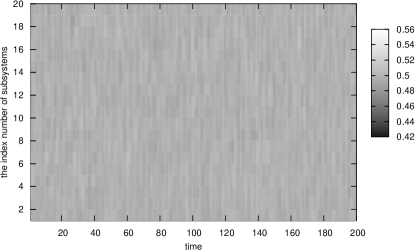
Figure 1: Time evolution of macroscopic observables $F_{l}(n)$. ($\epsilon=10^{-3},N=10^{4},K=100,L=20$. Left : $B=1.5$, right : $B=3.0$.) The degree of $F_{l}(n)$ is represented by its thickness.

3 Discussion

We defined the equilibrium and non-equilibrium states in dynamical systems. In this context, the ergodic measure in infinite measure systems is one of the measures characterizing the non-equilibrium non-stationary state, because macroscopic observables, which are the result of the time average of microscopic observables, are intrinsically random. In fact, the numerical simulation of the coupled modified Bernoulli map lattice has provided a non-equilibrium non-stationary state clearly in the infinite measure case.

References

- Birkhoff (1931) G. D. Birkhoff, Proc. Natl. Acad. Sci. USA 17, 656–660 (1931).
- Aaronson (1997) J. Aaronson, An Introduction to Infinite Ergodic Theory, American Mathematical Society, Province, 1997.
- Thaler (1998) M. Thaler, Trans. Am. Math. Soc. 350, 4593–4607 (1998).
- Thaler (2002) M. Thaler, Ergod. Theory Dyn. Syst. 22, 1289–1312 (2002).
- Thaler and Zweimüller (2006) M. Thaler, and R. Zweimüller, Probab. Theory Relat. Fields 135, 15–52 (2006).
- Akimoto (2008) T. Akimoto, J. Stat. Phys. 132, 171–186 (2008).