Modal Analysis and Coupling in
Metal-Insulator-Metal Waveguides

Abstract

This paper shows how to analyze plasmonic metal-insulator-metal waveguides using the full modal structure of these guides. The analysis applies to all frequencies, particularly including the near infrared and visible spectrum, and to a wide range of sizes, including nanometallic structures. We use the approach here specifically to analyze waveguide junctions. We show that the full modal structure of the metal-insulator-metal (mim) waveguides—which consists of real and complex discrete eigenvalue spectra, as well as the continuous spectrum—forms a complete basis set. We provide the derivation of these modes using the techniques developed for Sturm-Liouville and generalized eigenvalue equations. We demonstrate the need to include all parts of the spectrum to have a complete set of basis vectors to describe scattering within mim waveguides with the mode-matching technique. We numerically compare the mode-matching formulation with finite-difference frequency-domain analysis and find very good agreement between the two for modal scattering at symmetric mim waveguide junctions. We touch upon the similarities between the underlying mathematical structure of the mim waveguide and the $\mathcal{PT}$ symmetric quantum mechanical pseudo-Hermitian Hamiltonians. The rich set of modes that the mim waveguide supports forms a canonical example against which other more complicated geometries can be compared. Our work here encompasses the microwave results, but extends also to waveguides with real metals even at infrared and optical frequencies.

I Introduction

Waveguides have long been used to controllably direct energy flow between different points in space. Understanding the way waves propagate in waveguides led to a multitude of creative designs—all the way from the pipe organ to light switches used in fiber optic communications. In optics, recently there has been a growing interest in making use of the dielectric properties of metals to guide electromagnetic energy by using sub-wavelength sized designs that work in the infrared and the visible bands of the spectrum. One of the motivations for doing photonic research using metals is to find the means to integrate electronic devices with sizes of tens of nanometers with the relatively much larger optical components—so that some of the electrons used in the communication channels between electrical circuitry can be replaced by photons for faster and cooler operation Ozbay2006.

Whereas the use of metals for directing electromagnetic energy is relatively new in optics, sub-wavelength guiding of light by metals is the norm in the microwave domain. Even though the permittivity of metals can be large in magnitude at both microwave and optical frequencies, the characteristics of the permittivity are quite different in the two frequency regimes.

In the microwave regime, electrons go through multiple collisions with the ions of the lattice during an electromagnetic cycle according to the phenomenological Drude model of electrons. Therefore, the electron movement is a drift motion where the velocity of electrons is proportional to the applied field strength (Ref. Ashcroft1976, Chp. 1). As a result, the induced dipole moment density and hence the permittivity is a large, negativefootnote_1 imaginary number. On the other hand, at optical frequencies below the plasma oscillation frequency, electrons go through a negligible number of collisions during an electromagnetic cycle and this time acceleration of electrons is proportional to the applied field strength which then results in a permittivity that can be substantially a large real negative number. Above the plasma frequency, the induced dipole moment density is very low and the permittivity is predominantly a positive real number less than one (Ref. Bohren1983, Chp. 9).

The dielectric slab and the parallel plate (i.e. consisting of two parallel perfectly conducting metal plates) waveguides are the two canonical examples of waveguiding theory. If we have a layered metal-insulator-metal (mim) geometry, it is possible to smoothly transition from the dielectric slab to the parallel plate waveguide by reducing the frequency of operation, and therefore varying the metallic permittivity $\epsilon_{m}$.

At frequencies above the plasma frequency, the metal has a permittivity $\epsilon_{m}<1$ whereas the insulator has $\epsilon_{i}\geq 1$. We illustrate the geometry in the inset of Fig. 1.

The physical modes that the dielectric slab waveguide supports fall into two sets: guided modes and radiation modes (Ref. Marcuse1991, Chp. 1). Guided modes consist of a countable, finite set, i.e. there is only a finite number of discrete guided modes. Radiation modes consist of a non-countable, infinite set, i.e. they form a continuum. The combination of these two sets of modes form a complete and orthogonal basis set.

Now suppose that we change our operation frequency to one which is very close to the dc limit where $\epsilon_{m}$ is an arbitrarily large, negative, imaginary number. In this limit, we can approximate the metal as a perfect electric conductor (pec) where $|\epsilon_{m}|\rightarrow\infty$. Such an approximation then gives us the parallel plate waveguide of the microwave domain. Unlike the dielectric slab, the parallel plate geometry is bounded in the transverse dimension—fields are not allowed to penetrate into the pec. There are infinitely many discrete modes of the parallel plate, all of which have sinusoidal shapes, and there are no continuum modes. The collection of the infinitely many discrete modes forms a complete orthogonal basis set.

In this paper we will investigate the modal structure of the two dimensional mim waveguide in the infrared regime where $\epsilon_{m}$ is primarily a large, negative real number. The geometry of the mim waveguide is exactly the same as the one in the inset of Fig. 1. The only difference between the parallel plate, mim and the dielectric slab waveguides is in the numerical value of $\epsilon_{m}$, which depends on the frequency of operation.

There have been numerous studies of the mim waveguide in the literatureDavis1965; Davis1966; Economou1969; Takano1972; Kaminow1974; Prade1991; Villa2001; Qing2005; Dionne2006; Ginzburg2006; Kim2006a; Gordon2006; Feigenbaum2007a; Kurokawa2007; Wang2007; Sun2007; Zakharian2007; Sturman2007. The fact that light can be guided within a deep subwavelength volume over a very wide range of wavelengths is one of the primary reasons why the mim geometry has attracted so much attention. The full set of modes that the mim waveguide supports—real and complex discrete modes as well as a continuous set of modes—has only very recently been publishedSturman2007. For other geometries, it has been shown that, in general, waveguides support real, complex and continuous sets of modesTamir1963; Paiva1991; Jablonski1994; Shu2006; Kim2006. In this work, we will provide the detailed mathematical framework to analyze the modal structure of the mim waveguide and emphasize how it is a hybrid between the parallel plate and the dielectric slab waveguides.

Operator theory will be the basis of the mathematical tool set with which we will analyze mim waveguides. In Section ii, we will introduce the notation and make some definitions pertaining to the operators in infinite dimensional spaces. In Section iii we will derive the discrete and continuum modes supported by the mim waveguide and show that the underlying operators are pseudo-Hermitian. In Section iv we will demonstrate that the modes we report form a complete basis set via example calculations using the mode-matching technique. In Section v we will discuss our results and underline some of the relevant developments in mathematics from both quantum mechanics and microwave theory with the hope of expanding our tools of analysis. Lastly, in Section vi we will draw our conclusions.

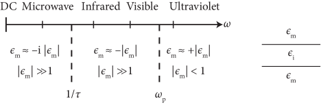
Figure 1: The change in the metallic permittivity $(\epsilon_{m})$ as the frequency of operation $(\omega)$ is varied leads to an evolution from the parallel plate waveguide at low frequencies to the dielectric slab waveguide at high frequencies for the two dimensional metal-insulator-metal geometry. We are assuming that $\epsilon_{m}$ is a Drude model metal where $\tau$ is the average time between collisions among the ions of the lattice and the free electrons, $\omega_{p}$ is the plasma oscillation frequency.

II Some Definitions

Throughout the paper, we will be using nomenclature from operator theory. In this section, we will define the terminology and introduce the notation which will be used in the following sectionsfootnote_2. The reader well versed in operator theory can directly skip to the next section.

A linear vector space is a space which is closed under the operations of addition and of multiplication by a scalar. We will call the elements of the space vectors. Spaces need not be finite dimensional—infinite dimensional vector spaces are also possible. For instance, the collection of all square integrable functions $f(x)$ defined on an interval $a<x<b$ forms an infinite dimensional vector space.

The inner product is a scalar valued function of two vectors $f$ and $g$, written $\langle f|g\rangle$ with the following properties ⟨f — g⟩=&⟨g — f⟩^*
⟨α_1 f + α_2 g — h⟩ =α_1^*⟨f — h⟩ + α_2^*⟨g — h⟩
⟨f — f⟩ ¿ 0   if $f\neq 0$. Here $(\cdot)^{*}$ denotes complex conjugation, $\alpha_{\{1,2\}}$ are arbitrary complex numbers and $f$, $g$, $h$ denote arbitrary members of the linear vector space $\mathcal{S}$.

For the infinite dimensional vector space of square integrable functions one possible definition of the inner product is ⟨f — g⟩=∫_a^b f^*(x) g(x)  dx. A linear vector space with an inner product is called an inner product space. In such spaces the norm of a vector $f$ is defined as f = ⟨f — f⟩. This is also known as the $\mathcal{L}^{2}$ norm, to denote square integrability in the sense of Lebesgue. By using the norm of a vector space, we can define the distance between its vectors $f$ and $g$ as $d(f,g)=\lVert f-g\rVert$ which is always nonzero if $f\neq g$. Here, $d(f,g)$ is called the metric—the measure of distance between vectors—of the inner product space. Suppose that $\mathcal{F}$ and $\mathcal{G}$ are two subsets of the inner product space $\mathcal{S}$ and that $\mathcal{F}$ is also a subset of $\mathcal{G}$, i.e. $\mathcal{F}\subset\mathcal{G}\subset\mathcal{S}$. $\mathcal{F}$ is said to be dense in $\mathcal{G}$, if for each $g\in\mathcal{G}$ and $\varepsilon>0$, there exists an element $f\in\mathcal{F}$ where $d(f,g)<\varepsilon$ (Ref. Hanson2002, pp. 94–95).

A vector space $\mathcal{S}$ is complete if all converging sequences of vectors $f_{n}(x)$ converge to an element $f\in\mathcal{S}$. An inner product space which is complete when using the norm defined by eq2-eq3 is called a Hilbert space.

An operator $\mathsf{L}$ is a mapping that assigns to a vector $f$ in a linear vector space $\mathcal{S}_{1}$ another vector in a different vector space $\mathcal{S}_{2}$ which we denote by $\mathsf{L}f$ (most often $\mathcal{S}_{1}=\mathcal{S}_{2}$). An operator is linear if $\mathsf{L}(\alpha_{1}f+\alpha_{2}g)=\alpha_{1}\mathsf{L}f+\alpha_{2}\mathsf{L}g$ for arbitrary scalars $\alpha_{\{1,2\}}$ and vectors $f$, $g$. The domain of an operator $\mathsf{L}$ is the set of vectors $f$ for which the mapping $\mathsf{L}f$ is defined. The range of an operator $\mathsf{L}$ is the set of vectors $g=\mathsf{L}f$ for all possible values of $f$ in the domain of $\mathsf{L}$. A linear operator is bounded if its domain is the entire linear space $\mathcal{S}$ of vectors $f$ and if there exists a single constant $C$ such that $\lVert\mathsf{L}f\rVert<C\lVert f\rVert$. Otherwise the operator is unbounded. The differential operator is a classical example of an unbounded operator (Ref. Kreyszig1978, pp. 93–94). $\mathsf{L}$ is positive (negative) definite if $\langle f|\mathsf{L}f\rangle>0$ $\bigl{(}\langle f|\mathsf{L}f\rangle<0\bigr{)}$ for all possible $f$. Otherwise, $\mathsf{L}$ is indefinite.

A linear bounded operator $\mathsf{L}^{\dagger}$ is said to be the adjoint of $\mathsf{L}$ if, for all $f$ and $g$ in $\mathcal{S}$ the condition $\langle g|\mathsf{L}f\rangle=\langle\mathsf{L}^{\dagger}g|f\rangle$ is satisfied. If $\mathsf{L}=\mathsf{L}^{\dagger}$ then $\mathsf{L}$ is said to be self-adjoint. If the operator $\mathsf{L}$ is unbounded, then the equality $\langle g|\mathsf{L}f\rangle=\langle\mathsf{L^{\dagger}}g|f\rangle$ defines a formal self-adjoint (Ref. Hanson2002, Sec. 3.4.1).

Suppose we have a set of orthonormal vectors $\{f_{n}\}$ which span the Hilbert space $\mathcal{H}$. Then, we can expand any vector $g\in\mathcal{H}$ as $g=\sum_{n}\langle f_{n}|g\rangle f_{n}$. Similarly, any linear bounded operator $\mathsf{L}$ acting on $g$ results in Lg = & ∑_n ⟨f_n — g⟩ L f_n = ∑_n,m ⟨f_n — g⟩ ⟨f_m — L f_n⟩ f_m
= ∑_m,n f_m ⟨f_m — L f_n⟩ ⟨f_n — g⟩ where we expanded $\mathsf{L}f_{n}$ in terms of the basis $\{f_{m}\}$ to get to the last line. Once we choose a complete orthonormal basis set, we can describe the action of $\mathsf{L}$ on any vector $g$ by the product of an infinite dimensional matrix with elements $\langle f_{m}|\mathsf{L}f_{n}\rangle$ and an infinite dimensional vector with elements $\langle f_{n}|g\rangle$—a generalization of regular matrix multiplication. The infinite dimensional matrix is called the representation of $\mathsf{L}$ in $\{f_{n}\}$. If the matrix for $\mathsf{L}$ is diagonal, then we call that the spectral representation (Ref. Friedman1990, p. 110).

The spectral representation for an operator $\mathsf{L}$ depends on the study of the inverse of the operator $\mathsf{L}-\lambda$, which we will denote by $(\mathsf{L}-\lambda)^{-1}$, for all complex values of $\lambda$ (Ref. Friedman1990, p. 125). Let the domain and range of $\mathsf{L}$ be denoted by $\mathcal{D}_{L}$ and $\mathcal{R}_{L}$. The point (discrete) spectrum is the set of $\lambda$ for which $(\mathsf{L}-\lambda)^{-1}$ does not exist. The continuous spectrum is the collection of $\lambda$ for which $(\mathsf{L}-\lambda)^{-1}$ exists and is defined on a set dense in $\mathcal{R}_{L}$, but for which it is unbounded. The residual spectrum is the collection of $\lambda$ for which $(\mathsf{L}-\lambda)^{-1}$ exists (it may or may not be bounded), but for which it is not defined on a set dense in $\mathcal{R}_{L}$. The spectrum of $\mathsf{L}$ consists of values of $\lambda$ which belong to either the point, continuous or the residual spectrum (Ref. Kreyszig1978, p. 371 and Ref. Locker2000, p. 21). We summarized the taxonomy of the spectrum in Fig. 2.

Figure 2: Classification of the spectrum for an operator in a general space. Point spectrum is sometimes called the discrete spectrum.

III Spectrum

After having defined the necessary terminology, in this section we will derive the modal structure (spectrum) of the mim waveguide. We will specifically focus on the even modes of the waveguide, for which the transverse magnetic (tm) field component is an even function of the transverse coordinate, $x$. The reason why we focus on even modes is that we will be analyzing the scattering of the main, even mode of the mim waveguide—which is also a tm mode—off of a symmetric junction with a different sized mim waveguide. Due to the symmetry of the problem at hand, even modes will be sufficient. We could also solve for the case of the odd modes by a similar approach, but we omit that explicit solution for reasons of space. Evenness of the function is achieved by putting a fictitious perfect electric conductor (pec) at the $x=0$ plane of the waveguide, which forces the tangential electric field $E_{z}$ to be an odd function, and the magnetic field $H_{y}$ to be an even function of $x$. In other words, the modes of this fictitious waveguide with the pec at $x=0$ are mathematically the same as the even modes of the actual waveguide of interest, and so we will work with this hypothetical waveguide for our mathematics. The geometry is as shown in Fig. 3. $\epsilon_{m}$ refers to the permittivity of the metal region and $\epsilon_{i}$ of the insulator region. At infrared frequencies, $\epsilon_{m}$ is a complex number with a large, negative real part and a relatively small imaginary part (the sign of which is determined by the time convention used, being negative for an $\exp(\mathrm{i}\omega t)$ time dependence).

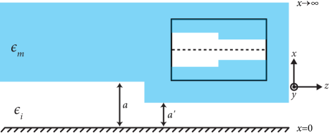
Figure 3: (Color online) Geometry for the even modes of the mim waveguide. The $x=0$ plane contains a fictitious perfect electric conductor to simplify the problem when dealing only with even tm modes of the guide. This fictitious mim waveguide is equivalent to an actual guide with an insulator thickness of $2a$. The inset shows the equivalent symmetric junction of two mim waveguides. The dashed line in the inset is the plane of symmetry, which is where the fictitious pec layer is introduced.

Let us begin with Maxwell’s equations for fields that have an $\exp(\mathrm{i}\omega t)$ time dependence.

$$\split\aligned\nabla\times\mathbf{E}(\mathbf{r})={}&-\mspace{-18mu}\mathrm{i}\omega\mu(x)\mathbf{H}(\mathbf{r})\\ \nabla\times\mathbf{H}(\mathbf{r})={}{}\mspace{-18mu}\mathrm{i}\omega\epsilon(x)\mathbf{E}(\mathbf{r}).$$ (1)

The mim waveguide is a two dimensional structure which does not have any variation in the $y$ direction. Therefore, we can eliminate all the derivatives with respect to $y$ in Maxwell’s equations. Furthermore, our study will be based on the tm modes which only have the $H_{y}$, $E_{x}$ and $E_{z}$ field components. Also, the uniformity of the waveguide in the $z$ direction leads to $\exp(-\mathrm{i}k_{z}z)$ as the space dependence in $z$ by using the separation of variables technique for differential equations ($k_{z}$ may, however, be a complex number). After simplifying the curl equations in eq5, we have the following relationships between the different field components iωμ(x) H_y(x) =& ik_z E_x(x) + ddx E_z(x)
ik_z H_y(x) = iωϵ(x) E_x(x)
ddxH_y(x) = iωϵ(x) E_z(x). Using these equations we get the following differential equation for $H_{y}$ (ϵ(x) ddx 1ϵ(x) ddx + ω^2 μ(x) ϵ(x) )H_y = k_z^2 H_y and since $E_{z}(0)=0$ by the pec wall at $x=0$, the boundary condition for $H_{y}$ under eq6 becomes $\left.\frac{\,\mathrm{d}}{\,\mathrm{d}x}H_{y}(x)\right|_{x=0}=0$. The equation eq7 is in the Sturm-Liouville form (Ref. Hanson2002, ch. 5).

III.1 Point Spectrum

The standard approach (Ref. Hanson2002, Chap. 5) in the calculation of the point spectrum of a Sturm-Liouville equation as in eq7 starts with a redefinition of the space to $\mathcal{L}^{2}_{\epsilon}$—the set of all weighted Lebesgue square-integrable functions such that ∫f(x)^21ϵ(x)  dx ¡ ∞ which implies that the boundary condition at infinity should be $\lim_{x\rightarrow\infty}H_{y}(x)=0$. The inner-product in $\mathcal{L}^{2}_{\epsilon}$, denoted by $\langle\!\langle\cdot|\cdot\rangle\!\rangle_{\epsilon}$, is then defined as ⟨​⟨f — g⟩​⟩_ϵ=∫f^*(x)g(x) 1ϵ(x) dx. In order to have a definite metric for $\mathcal{L}^{2}_{\epsilon}$, the inner product should be such that $\langle\!\langle f|f\rangle\!\rangle_{\epsilon}>0$ for all $f\neq 0$ so that the norm of any non-zero vector will be a positive quantity. This in turn implies that to have a definite metric, $\epsilon(x)$ should be a real and positive number for all $x$. Within the Hilbert space obtained by our choice of the inner product $\langle\!\langle\cdot|\cdot\rangle\!\rangle_{\epsilon}$, we can write eq7 as $\mathsf{L}H_{y}=k_{z}^{2}H_{y}$. The operator L = ϵ(x) ddx 1ϵ(x) ddx + ω^2 μ(x) ϵ(x) is self-adjoint since $\langle\!\langle f|\mathsf{L}g\rangle\!\rangle_{\epsilon}=\langle\!\langle\mathsf{L}f|g\rangle\!\rangle_{\epsilon}$ for all $f$ and $g$ as long as $\epsilon(x)\in\mathbb{R}$ and $\epsilon(x)>0$. One can then easily prove that the point spectrum of $\mathsf{L}$ is purely real (Ref. Churchill1941, p. 50). The lossless dielectric slab waveguide, which satisfies all the criteria we mentioned, therefore has a purely real point spectrum.

Unfortunately, the arguments above fail for the mim waveguide system since the condition $\epsilon(x)>0$ is no longer satisfiedSturman2007. The dielectric constants of metals can have negative real parts at some frequencies (e.g., in the infrared and visible regions), and generally also have imaginary components corresponding to loss, especially at optical frequencies. We will now separately analyze the lossy and the lossless metal cases.

III.1.1 Lossless Case

Since $\lvert\Imag(\epsilon_{m})\rvert\ll\lvert\Real(\epsilon_{m})\rvert$ at infrared frequencies, it is worthwhile investigating the case of real, negative permittivity, i.e., $\epsilon_{m}=-\lvert\epsilon_{m}\rvert$. The standard Sturm-Liouville theory is not applicable in this case, because it requires the weighting function $\epsilon(x)$ to have the same sign over its entire domain of definition (Ref. Churchill1941, p. 50). However, $\epsilon_{i}>0$ whereas $\epsilon_{m}<0$ for the mim waveguide, under the approximation of negligible loss. The definition of the inner-product eq8 becomes indefinite in this case, since we can have $\langle\!\langle f|f\rangle\!\rangle_{\epsilon}\leq 0$ for some $f\neq 0$. As a result, we no longer can operate in the Hilbert space. The space of functions with an indefinite metric is called the Krein space. In contrast to the Hilbert space case, the spectrum of the self-adjoint operators in Krein spaces is, in general, not real (Ref. Zettl2005, p. 220). An early analysis of a real Sturm-Liouville equation with a complex point spectrum can be found in Ref. Richardson1918.

To prove that eq7 accepts complex solutions even when $\epsilon(x)\in\mathbb{R}$, let us work in the well defined $\mathcal{L}^{2}$ space with an inner-product as defined in eq2. Because $\langle\cdot|\cdot\rangle$ is always definite, we are back in the Hilbert space, but $\mathsf{L}$ is no longer self-adjoint in $\mathcal{L}^{2}$. Two integrations by partsfootnote_3 give $\mathsf{L}^{\dagger}$ as L^†= ddx 1ϵ(x) ddx ϵ(x) + ω^2 μ(x) ϵ(x) with boundary conditions

$$\aligned H_{y}(x)&\Bigr{|}_{x\rightarrow\infty}\mspace{-18mu}=0\\ \frac{\,\mathrm{d}}{\,\mathrm{d}x}\epsilon(x)H_{y}(x)\Bigr{|}_{x=0}\mspace{-18mu}=0.$$

We see that $\mathsf{L}^{\dagger}=\epsilon^{-1}\mathsf{L}\epsilon$ which makes $\mathsf{L}$ by definition pseudo-Hermitian Mostafazadeh2002b; Mostafazadeh2008. It has been proved that a pseudo-Hermitian operator does not have a real spectrum if $\mathcal{L}^{2}_{\epsilon}$ is indefinite (Ref. Mostafazadeh2002b, Th. 3).

Alternatively, we can approach the problem by defining L^′= ddx 1ϵ(x) ddx + ω^2 μ(x) and rewriting eq7 as L^′H_y = kz2ϵ H_y. Using eq2 it can be shown that $\mathsf{L}^{\prime}$ is self-adjoint in $\mathcal{L}^{2}$ so that ⟨H_y2 — L^′H_y1⟩ = ⟨L^′H_y2 — H_y1⟩ which leads to the generalized eigenvalue problem for the self-adjoint operators $\mathsf{L}^{\prime}$ and $\mathsf{\epsilon}^{-1}$ as L^′H_y = k_z^2 ϵ^-1 H_y where $k_{z}^{2}$ is the eigenvalue. The point spectrum of the self-adjoint generalized eigenvalue problem will be complex only if both $\mathsf{L}^{\prime}$ and $\mathsf{\epsilon}^{-1}$ are indefinite (Ref. Mrozowski1997, p. 38). The indefiniteness of $\mathsf{\epsilon}^{-1}$ is trivial because epsilon can be a positive or negative quantity now. To show that $\mathsf{L}^{\prime}$ is indefinite, observe that by using the boundary conditions in integration by parts, one can get ⟨H_y — L^′H_y⟩ = ∫_0^∞( ω^2 μH_y(x)^2 - 1ϵ(x) —dHy(x)dx—^2 )  dx which can be positive or negative depending on the choice of $H_{y}(x)\in\mathcal{L}^{2}$. Therefore, $\mathsf{L}^{\prime}$ is indefinite, and $k_{z}^{2}$ will accept complex values. Note that the classification of the point spectrum into the real and the complex categories is based on $k_{z}^{2}$ and not $k_{z}$. Hence, the set of modes with purely real and negative $k_{z}^{2}$—which leads to a purely imaginary $k_{z}$—are categorized as real modes in this approach.

III.1.2 Lossy Case

As we mentioned earlier, $\epsilon_{m}$ has an imaginary part. As a result, for those cases when neglecting the imaginary part of $\epsilon_{m}$ is not desired, $\mathsf{L}$ cannot be made self-adjoint by a redefinition of the inner-product. Therefore, the point spectrum—the set of $k_{z}^{2}$ for which $(\mathsf{L}-k_{z}^{2})$ does not have an inverse—will be complex. A general classification of the spectrum for non-self-adjoint operators is still an open problem (Ref. Zettl2005, p. 301 and Ref. Davies2002). Also, completeness of the spectrum is difficult to prove. However, the mim waveguiding problem can be shown to have a spectrum which forms a complete basis set even when $\mathsf{L}$ is non-self-adjoint (Ref. Hanson2002, pp. 333-334, Th. 5.3).

III.1.3 Mode Shape

The dispersion equation that should be solved in order to find the $k_{z}$ values for the modes of the mim waveguide is derived by satisfying the continuity of tangential electric and magnetic fields at material boundaries and applying the boundary conditions. We refer the reader to Ref. Hanson2002, pp. 462–470 and Refs. Economou1969; Prade1991; Dionne2006; Feigenbaum2007a; Zakharian2007; Sturman2007 for the details. The eigenvectors $(\psi_{n})$ and the dispersion equation for the corresponding eigenvalues $(k_{z,n}^{2})$ of eq7 for the even tm modes of the mim waveguide are ψ_n(x)= & H_0 {cosh(κi,nx)cosh(κi,na ) 0¡x¡a
e ^-κ_m,n (x-a) a¡x¡∞
tanh(κ_i,n a) = - κm,n/ϵmκi,n/ϵi
k_z,n^2 = κ_m,n^2 + ω