Geometrical Rabi transitions between decoupled quantum states

Abstract

A periodic perturbation such as a laser field cannot induce transitions between two decoupled states for which the transition matrix element vanishes. We show, however, that if in addition some system parameters are varied adiabatically, such transitions become possible via adiabatic-change-induced excitations to other states. We demonstrate that full amplitude transfer between the two decoupled states can be achieved, and more significantly, the evolution of the system only depends on its path in parameter space. Our technique then provides a valuable means of studying nontrivial geometrical dynamics via auxiliary states with large energy splittings.

Central to the spirit of quantum mechanics are the concepts of discrete quantum states and the transitions between them. To induce coherent quantum transitions between two nondegenerate states, the most often used technique is to apply an in-resonance periodic perturbation such as a laser or microwave field. This induces Rabi oscillations ref:QO if the transition matrix element of the perturbation Hamiltonian between the two states is non-vanishing. Rabi transitions are efficient in the sense that full amplitude transfer can be achieved if the periodic perturbation is exactly in resonance. A different way of inducing quantum transitions is by adiabatically varying some parameters in the system Hamiltonian ref:Messiah . This makes the eigenstates of the system time dependent and causes a system initially prepared in one eigenstate to transition to other states. Though inefficient in exciting the system out of its initial state, adiabatic-change-induced quantum transitions have some intriguing properties. In some important contexts such as charge transfer via quantum pumping ref:Thouless83 in solid-state physics, the system dynamics turn out to be geometrical, depending only on the path traversed in parameter space and thus allowing robust control of the system and precise transfer of charge.

In this work we consider the possibility of Rabi transitions between two decoupled (and nondegenerate) quantum states, a problem of both theoretical interest and practical significance. One such example is the double-well potential depicted in Fig. 1 (a) which has two localized states $\Phi_{0}(x)$ and $\Phi_{2}(x)$ (with energies $E_{0}$ and $E_{2}$). Physical realizations of such a situation can be a double-well quantum dot system ref:Qdot , an SQUID system biased close to half flux quantum ref:Squid , or an atomic system trapped in an optically engineered potential ref:BEC . If we apply a resonant periodic perturbation to a system with two decoupled states, direct quantum transitions cannot occur because the transition matrix element vanishes (which is the definition of “decoupled”). In the double-well potential system in Fig. 1 (a), this is manifested by the fact that a resonant perturbation $H^{\prime}(x)\cos(E_{2}-E_{0})t/\hbar$ has no effect since $H^{\prime}_{02}=0$ (which follows from the fact that $\Phi_{0}(x)$ and $\Phi_{2}(x)$ do not overlap). Nevertheless, we explore the interesting possibility of adiabatically changing some parameters of the system Hamiltonian, in addition to applying a resonant periodic perturbation. We will see that, by making use of inefficiently-excited auxiliary states, full amplitude transfer between the two decoupled states can be achieved. More significantly, the system dynamics is geometrical, meaning it is dictated by rotation angles determined by the path the system traversed in parameter space only and does not depend on time explicitly.

Figure 1: (a) Two localized and non-overlapping states $\Phi_{0}$ and $\Phi_{2}$ in a double-well potential. Here $x$ is the coordinate of the physical system under consideration (e.g., position for a quantum dot system and flux for a SQUID system). (b) Nondegenerate model system consisting of two decoupled states 0 and 2 and auxiliary state 1. The periodic perturbation is in resonance with the 0-2 transition but off resonance with 0-1 and 1-2 transitions.

We start by considering the simplest setup that consists of three nondegenerate states as shown in Fig. 1 (b). These are assumed to be a subspace of a system with unperturbed Hamiltonian $H_{0}(\bm{\lambda})$. Here, $\bm{\lambda}$ is a collection of parameters. The eigenenergies and eigenstates of $H_{0}(\bm{\lambda})$ are $E_{n}(\bm{\lambda})$ and $\Phi_{n}(\bm{\lambda})$: $H_{0}(\bm{\lambda})\Phi_{n}(\bm{\lambda})=E_{n}(\bm{\lambda})\Phi_{n}(\bm{\lambda})$, where $n$ is a set of quantum numbers to label the spectrum of the system. We will use $n=0,1,2$ to label our three state system. All other states are assumed to be energetically far away from our three-state subspace and do not need to be considered for our problem.

We apply to the system a (quasi) periodic perturbation $H^{\prime}(t)=2H^{\prime}(\bm{\lambda})cos(\int\omega(t)dt)$ in resonance with state 0 and 2. However, as discussed before, we assume that these two states are decoupled, $\langle\Phi_{0}|H^{\prime}|\Phi_{2}\rangle=0$. The slow time varying frequency $\omega(t)$ of the perturbation is close to the energy difference between state 0 and 2. Such quasi periodic perturbation can be realized, for instance, by applying a laser or microwave with a time varying phase. The Hamiltonian of the 3 state system is then

$$H=\sum_{j=0}^{2}E_{j}(\bm{\lambda})|\Phi_{j}(\bm{\lambda})\rangle\langle\Phi_{j}(\bm{\lambda})|+2H^{\prime}cos(\int\omega(t)dt).$$ (1)

Since state 0 and 2 are decoupled, the periodic perturbation, though in resonance, cannot induce Rabi oscillations between them. To facilitate possible transitions between state 0 and 2, we slowly vary the parameters in the system Hamiltonian $H_{0}(\bm{\lambda})$, making $\bm{\lambda}=\bm{\lambda}(t)$ time dependent. When we use the Schrödinger equation to solve for the wave function of the system, $\psi(t)=\sum_{j=0}^{2}c_{j}(t)\Phi_{j}(\bm{\lambda}(t))$, the time dependence of the basis states must be taken into account. Assuming there is no Berry phase ($\langle\Phi_{j}(\bm{\lambda})|\dot{\Phi}_{j}(\bm{\lambda})\rangle=0$, $\dot{\Phi}_{j}$ the time derivative of ${\Phi}_{j}$) ref:Thouless83 , we derive

$$i\hbar\frac{d}{dt}\left(\begin{array}[]{c}c_{0}\\ c_{1}\\ c_{2}\end{array}\right)=\left(\begin{array}[]{ccc}E_{0}(\bm{\lambda})&H^{\prime}_{01}(t)-i\hbar\langle\Phi_{0}|\dot{\Phi}_{1}\rangle&0\\ H^{\prime}_{10}(t)-i\hbar\langle\Phi_{1}|\dot{\Phi}_{0}\rangle&E_{1}(\bm{\lambda})&H^{\prime}_{12}(t)-i\hbar\langle\Phi_{1}|\dot{\Phi}_{2}\rangle\\ 0&H^{\prime}_{21}(t)-i\hbar\langle\Phi_{2}|\dot{\Phi}_{1}\rangle&E_{2}(\bm{\lambda})\end{array}\right)\left(\begin{array}[]{c}c_{0}\\ c_{1}\\ c_{2}\end{array}\right),$$ (2)

where $H^{\prime}_{1j}(\bm{\lambda})=\langle\Phi_{1}(\bm{\lambda})|H^{\prime}|\Phi_{j}(\bm{\lambda})\rangle$, $j=0,2$ is the transition matrix element between the auxiliary state $\Phi_{1}(\bm{\lambda})$ and the other two states. Since $\hbar\omega$ is close to $E_{2}-E_{0}$ and off resonance with $E_{1}-E_{0}$ and $E_{2}-E_{1}$, $H^{\prime}_{1j}\neq 0$ does not imply direct Rabi transitions between state $\Phi_{1}$ and $\Phi_{j}$. Notice the terms $\hbar\langle\Phi_{1}(\bm{\lambda})|\dot{\Phi}_{j}(\bm{\lambda})\rangle$ also couple $\Phi_{0}(\bm{\lambda})$ and $\Phi_{2}(\bm{\lambda})$ to the auxiliary state $\Phi_{1}(\bm{\lambda})$.

There are a few arguments that we can use to simplify the equations of motion and understand the system dynamics. First, the precise conditions for “adiabatic” change and “off resonance” transitions are specified as $|\hbar\langle\Phi_{j}|\dot{\Phi}_{1}\rangle/(E_{1}-E_{j})|$, $|H_{1j}^{\prime}/(|E_{1}-E_{j}|-\hbar\omega)|<<1$ for $j=0,2$. Under such conditions, the transitions from state 0 and 2 to state 1 due to adiabatic change of the system Hamiltonian and off-resonance Rabi oscillation are very inefficient. Consequently, the amplitude on state 1 remains small and follows those on state 0 and 2 adiabatically. Second, when we study the amplitudes on state 0 and 2, it is convenient to switch to the “rotating frame” defined by $a_{0}=c_{0}$, $a_{2}=\exp\{i\int\omega(t)t\}c_{2}$ (we have chosen $E_{0}$ as the reference energy). In doing so, we can use the rotating wave approximation to drop fast oscillating terms in the rotating frame. We are led to the following effective equations for the amplitudes on state 0 and 2:

$$i\hbar\frac{d\psi_{R}}{dt}=\left(\begin{array}[]{cc}\delta E_{0}(\bm{\lambda},t)&\hbar\kappa(\bm{\lambda},t)\\ \hbar\kappa(\bm{\lambda},t)^{*}&\delta E_{2}(\bm{\lambda},t)+\Delta\end{array}\right)\psi_{R}.$$ (3)

Here, the two component wavefunction $\psi_{R}=(a_{0},a_{2})^{T}$, the Stark shifts are given by $\delta E_{j}=\left[2|H^{\prime}_{1j}|^{2}+|\hbar\langle\Phi_{j}|\dot{\Phi}_{1}\rangle|^{2}\right]/(E_{j}-E_{1})$, $j=0,2$, the detuning by $\Delta=E_{2}-E_{0}-\hbar\omega$, and the effective Rabi frequency by

$$\kappa=\frac{i\langle\Phi_{0}|\dot{\Phi}_{1}\rangle\langle\Phi_{1}|H^{\prime}|\Phi_{2}\rangle}{E_{1}-E_{0}}+\frac{i\langle\Phi_{0}|H^{\prime}|\Phi_{1}\rangle\langle\Phi_{1}|\dot{\Phi}_{2}\rangle}{E_{1}-E_{2}}.$$ (4)

When there are more than one auxiliary states, their contributions can simply be summed.

If we choose the (time varying) frequency of the laser appropriately so that $\Delta=\delta E_{0}(\bm{\lambda},t)-\delta E_{2}(\bm{\lambda},t)$, the equal diagonal terms in Eq. (3) can be dropped because they give an unobservable overall phase to $\psi_{R}$. Using $\dot{\Phi}_{j}=\nabla_{\bm{\lambda}}\Phi_{j}\cdot d\bm{\lambda}/dt$, $j=1,2$, we can rewrite Eq. (3) as follows:

$$id\psi_{R}=\{[\operatorname{{\mathrm{R}e}}\bm{f}(\bm{\lambda})]\sigma_{x}-[\operatorname{{\mathrm{I}m}}\bm{f}(\bm{\lambda})]\sigma_{y}\}\psi_{R}\cdot d\bm{\lambda}.$$ (5)

Here, $\operatorname{{\mathrm{R}e}}\bm{f}$ and $\operatorname{{\mathrm{I}m}}\bm{f}$ are the real and imaginary part of $\bm{f}(\bm{\lambda})$, a function of the parameters $\bm{\lambda}$ only:

$$\bm{f}=\frac{i\langle\Phi_{0}|\nabla_{\bm{\lambda}}\Phi_{1}\rangle H^{\prime}_{12}}{E_{1}-E_{0}}+\frac{iH^{\prime}_{01}\langle\Phi_{1}|\nabla_{\bm{\lambda}}\Phi_{2}\rangle}{E_{1}-E_{2}}.$$ (6)

The intriguing dynamics described by Eqs. (5) and (6) are our main results. These equations describe the rotation of an effective spin 1/2 under the effective magnetic field determined by $\operatorname{{\mathrm{R}e}}\bm{f}$ and $\operatorname{{\mathrm{I}m}}\bm{f}$. However, remarkably, the evolution of the wavefunction is solely determined by the path of $\bm{\lambda}$ in the parameter space. Therefore, the system dynamics is geometrical (and non-Abelian in general), even though the Berry phase has been set to zero ($\langle\Phi_{j}(\bm{\lambda})|\dot{\Phi}_{j}(\bm{\lambda})\rangle=0$) ref:nonAbelian .

Formally, The solution of Eq. (5) is $\psi_{R}(t)=P\exp{\left(-i\int\{[\operatorname{{\mathrm{R}e}}\bm{f}(\bm{\lambda})]\sigma_{x}-[\operatorname{{\mathrm{I}m}}\bm{f}(\bm{\lambda})]\sigma_{y}\}\cdot d\bm{\lambda}\right)}\psi_{R}(0)$, where $P$ stands for path ordering. When $\langle\Phi_{0}|\nabla_{\bm{\lambda}}\Phi_{1}\rangle H^{\prime}_{12}$ and $H^{\prime}_{01}\langle\Phi_{1}|\nabla_{\bm{\lambda}}\Phi_{2}\rangle$ are real, Eq. (5) can be integrated explicitly. The solution is $\psi_{R}(t)=\exp{\left(-i\Gamma\sigma_{y}\right)}\psi_{R}(0)$, where $\Gamma$ is a geometrical angle determined by the path of the adiabatically varied parameters $\bm{\lambda}(t)$ only: $\Gamma=i\int\bm{f}(\bm{\lambda})\cdot d\bm{\lambda}$. The physics is similar to conventional resonant Rabi oscillation which can be understood in terms of an effective spin 1/2 rotating around the $y$ axis. However, rather than oscillating sinusoidally with time, the amplitudes on the two states are determined by a geometrical rotation angle not explicitly dependent on time. When the parameters undergo cyclic changes, their paths form closed loops in parameter space and the phase $\Gamma$ can be expressed as a surface integral using Stokes’s theorem. For instance, in the case of two adiabatically varied parameters, $\bm{\lambda}(t)=(\mu(t),\nu(t))$, which form a closed loop $C$ in the $\mu-\nu$ plane, $\Gamma$ can be expressed as

$$\bigcirc\int\int_{C}\left\{\left(\frac{\partial}{\partial\mu}\frac{H_{12}^{\prime}\langle\Phi_{0}|}{E_{1}-E_{0}}\right)\left|\frac{\partial\Phi_{1}}{\partial\nu}\right\rangle-\left(\frac{\partial}{\partial\nu}\frac{H_{12}^{\prime}\langle\Phi_{0}|}{E_{1}-E_{0}}\right)\left|\frac{\partial\Phi_{1}}{\partial\mu}\right\rangle\right\}$$

$$+\left\{\left(\frac{\partial}{\partial\mu}\frac{H_{01}^{\prime}\langle\Phi_{1}|}{E_{1}-E_{2}}\right)\left|\frac{\partial\Phi_{2}}{\partial\nu}\right\rangle-\left(\frac{\partial}{\partial\nu}\frac{H_{01}^{\prime}\langle\Phi_{1}|}{E_{1}-E_{2}}\right)\left|\frac{\partial\Phi_{2}}{\partial\mu}\right\rangle\right\}d\mu d\nu,$$

where $\bigcirc\int\int_{C}$ denotes the integral over a surface whose boundary is the closed parameter path $C$. When $\Gamma=\pi/2$, a system initially prepared in state 0 will evolve into state 2. Therefore, complete population transfer between these 2 states can be achieved, as in resonant Rabi transitions.

In the above, we have demonstrated that by using an auxiliary state and changing the parameters of the system Hamiltonian adiabatically, transitions between two decoupled quantum states can be induced. Remarkably, the resulting physics has advantages of both conventional Rabi oscillations and quantum pumping. It is possible to fully transfer the population between the two states, thus realizing efficient transitions. Moreover, the transition process is dictated by geometrical phases determined by the path of the adiabatically varied parameters only, and the speed with which the parameters are varied is irrelevant as long as the adiabatic conditions are satisfied. Our technique then provides a valuable means of studying nontrivial geometrical dynamics, with the aid of auxiliary states that have large energy splittings.

As a heuristic example, we consider a 1D problem of transferring a particle between two localized delta-function potential wells via extended states in a shallower square potential well. This is shown in Fig. 2 (a). The potential is given by $V(x)=-V_{c}\theta(a-|x|)-U_{l}\delta(x+a)-U_{r}\delta(x-a)$, where $\theta(x)$ is the unit step function, $2a$ is the distance between the two delta-function potential wells, and $V_{c}$ and $U_{(l,r)}$ (all positive) characterize the depths of the $c$entral, $l$eft and $r$ight potential wells. Such an idealized model with a small number of parameters can be used to approximate many physical systems such as a quantum dot or SQUID system with external biases to fine tune the potential.

Assuming the left delta-function well is the deepest, we define a unit length $\zeta=1/\gamma_{l}=\hbar^{2}/2mU_{l}$ ($m$ the “effective mass” of the particle), the extension of the wavefunction of an isolated delta-function potential well of depth $U_{l}$. When we choose $a=44\zeta$, $\gamma_{r}=2mU_{r}/\hbar^{2}=22/a$, $\beta=\sqrt{2mV_{c}}/\hbar=7.8/a$, the system has two localized bound states in the two delta-function potential wells and a few unlocalized bound states in the central well. Assuming the particle is initially in the left well, we transfer it to the right well by applying a periodic perturbation in resonance with the localized bound states and adiabatically varying the depths of the central and right wells.

We assume a dipolar-like interaction between the applied field (of strength $\mathcal{E}$) and the particle (with charge $q$). The field induced transition strength between states $i$, $j$ ($i,j$ = $l,c,r$) is then $H^{\prime}_{ij}=\mathcal{F}\cdot\langle x\rangle_{ij}$, where $\mathcal{F}=q\mathcal{E}$ and $\langle x\rangle_{ij}$ is the position matrix element evaluated between the two states. For the parameters we chose, $H^{\prime}_{lr}$ is negligibly small compared to $H^{\prime}_{lc}$ and $H^{\prime}_{rc}$. There is then no direct coupling between states in the delta-function wells and the transition between them occurs via coupling to the extended states in the central well. Assuming that the depths of the central and right wells are varied adiabatically and cyclically according to an elliptic path as depicted in Fig. 2 (b), we plot the effective Rabi frequency $\kappa$ during a cycle in Fig. 2 (c). Since $\kappa$ is real, the system will evolve like an effective spin 1/2 rotating around a fixed axis. $\kappa$ has a complicated time dependence, in contrast to conventional Rabi oscillations with constant Rabi frequencies. The total rotation angle per cycle, though, does not depend on the frequency at which the depths are varied. Plotted in Fig. 2 (d) is the rotation angle per cycle as a function of the size of the parameter path. Generally speaking, the transition is more efficient when the parameters are varied more in a cycle.

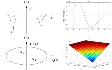
Figure 2: (a) Two delta-function potential wells with a square potential well in between. (b) The elliptic and adiabatic path for the depths of the central and right potential wells: $\varepsilon_{r}(t)=\hbar^{2}\gamma_{r}(t)^{2}/2m=\hbar^{2}\gamma_{r}^{2}/2m+\Lambda_{r}\cos\Omega t$, $\varepsilon_{c}(t)=\hbar^{2}\beta(t)^{2}/2m=\hbar^{2}\beta^{2}/2m+\Lambda_{c}\sin\Omega t$. (c) The effective Rabi frequency in one cycle for $\Lambda_{r}=0.037E_{u}$, $\Lambda_{c}=0.024E_{u}$ ($E_{u}=\hbar^{2}(\gamma_{r}^{2}-\beta^{2})/2m$ used as the energy scale), in unit of $\mathcal{F}\zeta\Omega/E_{u}$. Only the few lowest bound states in the central well with a substantial contribution are included. (d) The rotation angle $\Gamma$ per cycle for different values of $\Lambda_{r}$ and $\Lambda_{c}$, in unit of $\mathcal{F}\zeta/E_{u}$.

Our new quantum transition mechanism is a general principle not restricted to physical systems with localized states. As another example of its many possible applications, in the following we study a problem in which quantum interference plays an essential role. We consider a three-state system as shown in Fig. 3 (a). Here, the energies of the two ground states $|g_{1}\rangle$ and $|g_{2}\rangle$ are both close to $E_{g}$. The energy splitting and tunneling strength between them are $\varepsilon$ and $\delta$ which are assumed to be tunable. An example of such a system is a Josephson qubit ref:Squid where $\varepsilon$ and $\delta$ are determined by experimentally adjustable flux biases. The energy of an excited state $|e\rangle$, $E_{e}$, is high above that of the ground states, $E_{e}-E_{g}\gg\varepsilon,\delta$. Therefore the unperturbed Hamiltonian of the system is

$$H_{0}(\varepsilon,\delta)=\left(\begin{array}[]{ccc}E_{g}-\frac{\varepsilon}{2}&\frac{\delta}{2}&0\\ \frac{\delta}{2}&E_{g}+\frac{\varepsilon}{2}&0\\ 0&0&E_{e}\end{array}\right).$$ (7)

The upper-left block of the above Hamiltonian can be diagonalized to obtain two eigenstates $|g_{+}\rangle=\sin\alpha|g_{1}\rangle+\cos\alpha|g_{2}\rangle$, $|g_{-}\rangle=\cos\alpha|g_{1}\rangle-\sin\alpha|g_{2}\rangle$ with eigenenergies $E_{\pm}=E_{g}\pm\sqrt{\varepsilon^{2}+\delta^{2}}/2$, where $\alpha$ is defined by the relations $\cos 2\alpha=\varepsilon/\sqrt{\varepsilon^{2}+\delta^{2}}$ and $\sin 2\alpha=\delta/\sqrt{\varepsilon^{2}+\delta^{2}}$. If $\varepsilon$ and $\delta$ are varied adiabatically with time, these eigenstates and eigenenergies become time dependent.

Figure 3: (a) A three-state system consisting of two coupled ground states and an excited state. The energy difference $\varepsilon$ and tunneling strength $\delta$ between the ground states are tunable. (b) A cyclic and circular path $C$ of $\varepsilon$ and $\delta$ in parameter space.

We assume that the system is prepared in the state $|g_{-}\rangle$ and a periodic perturbation in resonance with $E_{e}-E_{-}$ is applied. The perturbative Hamiltonian is $H^{\prime}(t)=\bm{d}\cdot 2\bm{\mathcal{E}}\cos\int(E_{e}-E_{-})dt/\hbar$, where $\bm{d}$ and $\bm{\mathcal{E}}$ are the analogues of the “dipole moment” operator and “electric field.” We further assume that $\bm{d}_{eg_{1}}=\langle e|\bm{d}|g_{1}\rangle$ and $\bm{d}_{eg_{2}}=\langle e|\bm{d}|g_{2}\rangle$ are equal in magnitude and perpendicular in orientation: $|\bm{d}_{eg_{1}}|=|\bm{d}_{eg_{2}}|=d$ and $\bm{d}_{eg_{1}}\perp\bm{d}_{eg_{2}}$ ref:Note . If the angle between $\bm{d}_{eg_{2}}$ and the polarization of $\bm{\mathcal{E}}$ is $\beta$, we find $H^{\prime}_{eg_{-}}=\langle e|\bm{d}|g_{-}\rangle\cdot\bm{\mathcal{E}}=d\mathcal{E}\sin(\beta-\alpha)$ and $H^{\prime}_{eg_{+}}=\langle e|\bm{d}|g_{+}\rangle\cdot\bm{\mathcal{E}}=d\mathcal{E}\cos(\beta-\alpha)$, where $\mathcal{E}$ is the magnitude of the electric field. When we choose the polarization of the electric field such that $\beta=\alpha$, $H^{\prime}_{eg_{-}}=0$ and $H^{\prime}_{eg_{+}}=d\mathcal{E}$. In this case, $|g_{-}\rangle$ and $|e\rangle$ are decoupled due to the destructive interference. No transitions between these two states will occur even though the frequency of the periodic perturbation is in resonance with $E_{e}-E_{-}$.

In order to enable transitions between the two decoupled states $|g_{-}\rangle$ and $|e\rangle$, we adiabatically vary $\varepsilon(t)$ and $\delta(t)$. This will induce (inefficient) transitions from $|g_{-}\rangle$ to $|g_{+}\rangle$ which is coupled to $|e\rangle$. The condition for adiabaticity is $|\frac{\hbar\dot{\alpha}}{\sqrt{\varepsilon^{2}+\delta^{2}}}|\ll 1$. Meanwhile, we adjust the frequency of the periodic perturbation so that it remains in resonance with $E_{e}-E_{-}$, and rotate the polarization of the $\bm{\mathcal{E}}$ field so that $\beta(t)=\alpha(t)$. Though $|g_{-}(t)\rangle$ and $|e\rangle$ remain decoupled due to the destructive interference, transitions between them occur via adiabatic-change-induced excitation to $|g_{+}\rangle$. If the system is initially in $|g_{-}\rangle$, and $\varepsilon(t)$ and $\delta(t)$ undergo adiabatic and cyclic changes along path $C$ in parameter space, the amplitude in the excited state is $a_{e}=\sin{\Gamma}$, where $\Gamma$ is a geometrical rotation angle given by

$$\Gamma=-d\mathcal{E}\int\frac{d\alpha}{\sqrt{\varepsilon^{2}+\delta^{2}}}=\frac{d\mathcal{E}}{2}\bigcirc\int\int_{C}\frac{d\varepsilon d\delta}{(\varepsilon^{2}+\delta^{2})^{3/2}},$$ (8)

where $\bigcirc\int\int_{C}$ denotes the surface integral over the area bound by the closed path $C$. As an example, for a circular path of radius $\Lambda$ as depicted in Fig. 2 (b), $\Gamma=-\frac{d\mathcal{E}}{\Lambda}\Delta\alpha$, where $\Delta\alpha$ is the change of $\alpha$ along the path.

In conclusion, we have proposed a new mechanism for quantum transitions which is realized by simultaneously applying a resonant periodic perturbation and adiabatically changing the system parameters. This new mechanism allows to realize quantum transitions between decoupled states via inefficient excitations to auxiliary states. Remarkably, it combines the advantages of previously known methods, enabling efficient population transfer dictated by geometrical angles. Aside from its fundamental interest, our scheme is valuable for robust control of quantum transitions, and may find applications in quantum information processing.

We thank K. Das for helpful discussions. This work was partly supported by the Packard foundation. X. Z also acknowledges partial support from National Natural Science Foundation of China (grant No. 10875110).

References

(1) M. O. Scully and M. S. Zubairy, Quantum
Optics, Cambridge University Press, 1997.
(2) A. Messiah, Quantum Mechanics,
North-Holland, Amsterdam, 1962.
(3) D. J. Thouless, Phys. Rev. B 27, 6083
(1983).
(4) Y. Masumoto and T. Takagahara, Semiconductor
Quantum Dots, Springer, 2002.
(5) T. P. Orlando et al.,
Phys. Rev. B 60, 15398 (1999). J. E. Mooij et al.,
Science 285, 1036 (1999).
(6) S. Rolston, Phys. World 11, 27 (1998).
(7) M. V. Berry, Proc. R. Soc. Lond. A 392,
45 (1984). F. Wilczek and A. Zee, Phys. Rev. Lett. 52, 2111
(1984).
(8) We have made these assumptions to simplify our
results. The only condition required is that and
have different orientations.