Fermi Liquid parameters for dense nuclear matter in Effective Chiral Model

Abstract

We calculate relativistic Fermi liquid parameters (RFLPs) for the description of the properties of dense nuclear matter (DNM) using Effective Chiral Model. Analytical expressions of Fermi liquid parameters (FLPs) are presented both for the direct and exchange contributions. We present a comparative study of perturbative calculation with mean field (MF) results. Moreover we go beyond the MF so as to estimate the pionic contribution to the FLPs. Finally, we use these parameters to estimate some of the bulk quantities like incompressibility, sound velocity, symmetry energy etc. for DNM interacting via exchange of $\sigma$, $\omega$ and $\pi$ meson. In addition, we also calculate the energy densities and the binding energy curve for the nuclear matter. Results for the latter have been found to be consistent with two loop calculations reported recently within the same model.

I introduction

One of the most exciting field of contemporary nuclear research has been the studies of the properties of dense nuclear matter (DNM). Such studies are important both in the context of laboratory experiments and nuclear astrophysics. Therefore, several attempts have been made in recent years to ascertain the properties of nuclear system at densities higher than the normal nuclear matter densities [1, 2, 3, 4, 5, 6, 7].

The suitable description of nuclear matter at such high densities is provided by Quantum Hadrodynamics (QHD) [8]. Historically, QHD was developed by Walecka [9, 11, 10] to study the properties of neutron star where the nucleons are assumed to interact via the exchange of $\sigma$ and $\omega$ mesons. In this model starting with interacting Lagrangian the relativistic field equations are solved by making MF approximation where the meson fields are replaced by their vacuum expectation values. Subsequently, starting from the same model Chin developed a full diagrammatic scheme and showed that the MF results can be obtained by making Hartree approximation i.e. by retaining only the direct terms in a relativistic field theoretic approach [12]. In the same work, it was also shown how exchange corrections can be made and analytical expressions can be found for the energy density and related quantities by making some long range approximation for the $n-n$ interaction. Since then the QHD has undergone a series of developments which we do not discuss here but refer the reader to ref.[13, 14, 15, 16, 17, 18, 19].

The most recent model which we use here for the description of dense nuclear system is provided by the Chiral Effective Field theory (chEFT) [20, 21]. It might be recalled here, that, in such a framework, the explicit calculation of the Dirac vacuum is not required, rather, on the contrary, here, the short distance dynamics are absorbed into the parameters of the theory adjusted phenomenologically by fitting empirical data. For detail discussion refer the reader to ref. [21, 22, 23, 24]. Recently this model has been applied [23] to calculate the exchange corrections by evaluating nucleon loops involving $\sigma$, $\omega$ and $\pi$ as intermediate states, which we address here partly.

Our approach here is to study the dense nuclear system in terms of relativistic Fermi liquid parameters (RFLPs). Such an extention of the Fermi Liquid theory [25, 26] was first made by Baym and Chin in ref.[27]. It should, however, be noted that the calculation presented in ref.[27] were performed perturbatively where the original QHD model was used. It should, however, be noted that the first application of Fermi liquid theory (FLT) to study the nuclear system was due to Migdal [28] who used FLT to investigate the properties of unbound nuclear matter and finite nuclei [29]. FLT also provides theoretical foundation for the nuclear shell model [29] as well as nuclear dynamics of low energy excitations [26, 30]. The connection between Landau, Brueckner-Bethe and Migdal theories was discussed in ref.[31]. While these are all non-relativistic calculations, the relativistic calculations involving RFLT are rather limited.

After the original work of [27], the relativistic problem was revisited in [32] where one starts from the expression of energy density in presence of scalar and vector meson MF and takes functional derivatives to determine the FLPs. The results are found to be qualitatively different than the perturbative results [27, 32]. Moreover, besides $\sigma$ and $\omega$ meson, ref.[32] also includes the $\rho$ and $\pi$ meson and the model adopted was originally proposed by Serot that incorporates pion into the Walecka model. The latter, however, do not contribute to the parameters presented in [32] as the calculation was restricted only to the MF level where pion fails to contribute. On the other hand, the Migdal parameters using one-boson-exchange models of the nuclear force calculated in ref.[33, 34], in which a comparison of relativistic and non-relativistic results have also been studied.

In the present work, we use a model, where we have pions and we extend the calculation beyond MF to include the pionic contributions into the FLPs. Furthermore, we evaluate and compare the perturbative results with MF approximated results within the framework of the present model. In addition we also calculate various physical quantities like incompressibility, sound velocity and symmetry energy etc. Moreover, the results are compared whenever possible with the previous calculations by taking suitable limits. For instance, the exchange energy, we compare results calculated within the present scheme with a more direct evaluation of the loop diagrams like in ref.[23].

This paper is organized as follows. In Sec.II, we will depict brief outline of the formalism of FLT. We find the analytic expressions for the FLPs both for direct and exchange contributions in Sec.III. Subsequently, we determine chemical potential, energy density and various other thermodynamic quantities like incompressibility and sound velocity. Sec.IV, is devoted to calculate isovector LPs to which involves the $\pi$ meson contribution, and used to express the symmetry energy.

II Formalism

In FLT total energy $E$ of an interacting system is the functional of occupation number $n_{p}$ of the quasi-particle states of momentum $p$. The excitation of the system is equivalent to the change of occupation number by an amount $\delta n_{p}$. The corresponding energy of the system is given by [26, 27],

$${}E = E^{0}+\sum_{s}\int\frac{d^{3}{p}}{(2\pi)^{3}}\varepsilon_{ps}^{0}\delta n_{ps}+\frac{1}{2}\sum_{ss^{\prime}}\int\frac{d^{3}{p}}{(2\pi)^{3}}\frac{d^{3}{p^{\prime}}}{(2\pi)^{3}}f_{ps,p^{\prime}s^{\prime}}\delta n_{ps}\delta n_{p^{\prime}s^{\prime}},$$ (1)

where $E^{0}$ is the ground state energy and $s$ is the spin index, and the quasi-particle energy can be written as,

$$\varepsilon_{ps}=\varepsilon_{ps}^{0}+\sum_{s^{\prime}}\int\frac{d^{3}{p^{\prime}}}{(2\pi)^{3}}f_{ps,p^{\prime}s^{\prime}}\delta n_{p^{\prime}s^{\prime}},$$ (2)

where $\varepsilon_{ps}^{0}$ is the non-interacting single particle energy. The interaction between quasi-particles is given by $f_{ps,p^{\prime}s^{\prime}}$, which is defined to be the second derivative of the energy functional with respect to occupation functions,

$$f_{ps,p^{\prime}s^{\prime}}=\frac{\delta^{2}E}{\delta{n}_{ps}~{}\delta{n}_{p^{\prime}s^{\prime}}}.$$ (3)

Since quasi-particles are well defined only near the Fermi surface, one assumes

$$\left.\begin{array}[]{lll}&\varepsilon_{p}&=\mu+v_{f}(p-p_{f})\\ {\rm and}{}{}{}&p&\simeq p^{\prime}\simeq p_{f}.\end{array}\right\}$$ (6)

Then LPs $f_{l}$s are defined by the Legendre expansion of $f_{ps,p^{\prime}s^{\prime}}$ as [26, 27],

$$f_{l}=\frac{2l+1}{4}\sum_{ss^{\prime}}\int\frac{d\Omega}{4\pi}P_{l}(\cos\theta)f_{ps,p^{\prime}s^{\prime}},$$ (7)

where $\theta$ is the angle between $p$ and $p^{\prime}$, both taken to be on the Fermi surface, and the integration is over all directions of $p$ [27]. We restrict ourselves for $l\leq 1$ i.e. $f_{0}$ and $f_{1}$, since higher $l$ contribution decreases rapidly.

Now the Landau Fermi liquid interaction $f_{ps,p^{\prime}s^{\prime}}$ is related to the two particle forward scattering amplitude via [26, 27],

$$f_{ps,p^{\prime}s^{\prime}} = \frac{M}{\varepsilon_{p}^{0}}\frac{M}{\varepsilon_{p^{\prime}}^{0}}{\cal M}_{ps,p^{\prime}s^{\prime}},$$ (8)

where $M$ is the mass of the nucleon and the Lorentz invariant matrix ${\cal M}_{ps,p^{\prime}s^{\prime}}$ consists of the usual direct and exchange amplitude, which may be evaluated directly from the relevant diagrams as shown in Fig. 1 and Fig. 2.

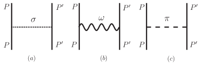
Figure 1: Schematic diagrams of direct contribution to forward scattering amplitude. Nucleons are represented by solid lines. $\sigma$, $\omega$ and $\pi$ mesons are denoted by dotted, wavy and dashed lines respectively.

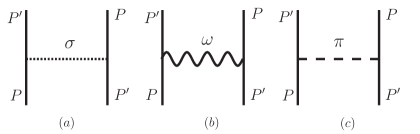
Figure 2: Schematic diagrams of exchange contribution to forward scattering amplitude. Nucleons are represented by solid lines. $\sigma$, $\omega$ and $\pi$ mesons are denoted by dotted, wavy and dashed lines respectively.

The spin averaged scattering amplitude $(f_{pp^{\prime}})$ is given by [27],

$$f_{pp^{\prime}} = \frac{1}{4}\sum_{ss^{\prime}}\frac{M}{\varepsilon_{p}^{0}}\frac{M}{\varepsilon_{p^{\prime}}^{0}}{\cal M}_{ps,p^{\prime}s^{\prime}}.$$ (9)

The dimensionless LPs are $F_{l}=N(0)f_{l}$, where $N(0)$ is the density of states at the Fermi surface defined as,

$$N(0) = \sum_{s}\int\frac{\rm d^{3}{p}}{(2\pi)^{3}}\delta(\varepsilon_{ps}-\mu)$$ (10)

$$= \frac{g_{s}g_{I}p_{f}^{2}}{2\pi^{2}}\left(\frac{\partial p}{\partial\varepsilon_{p}}\right)_{p=p_{f}}$$

$$\simeq \frac{g_{s}g_{I}p_{f}\varepsilon_{f}}{2\pi^{2}}.$$

Here $g_{s},g_{I}$ are the spin and isospin degeneracy factor respectively.

In the above expression $(\partial p/\partial\varepsilon_{p})_{p=p_{f}}$ is the inverse Fermi velocity $(v_{f}^{-1})$ related to the FL parameter $F_{1}$,

$$v_{f}^{-1}=(\partial p/\partial\varepsilon_{p})_{p=p_{f}}=(\mu/p_{f})(1+F_{1}/3).$$ (11)

With the help of Eq.(10) and Eq.(11) one writes [32]

$$\varepsilon_{f}=\mu(1+\frac{1}{3}F_{1}).$$ (12)

To compare Eq.(11) and Eq.(12) with the well known non-relativistic expressions one has to put $\varepsilon_{f}=M^{*}$ and $\mu=M$.

III Chiral Lagrangian and Landau parameters

We adopt the non-linear chiral model to calculate the FLPs and consequently estimate various quantities of physical interest like effective chemical potential, sound velocity, incompressibility, symmetry energy etc. Here all the fields are treated relativistically [27]. By retaining only the lowest order terms in the pion fields, one obtains the following Lagrangian from the chirally invariant Lagrangian [21, 23]:

$${\cal{L}} = \bar{\Psi}\left[\gamma^{\mu}(i\partial_{\mu}-g_{\omega}\omega_{\mu})-i\frac{g_{A}}{f_{\pi}}\gamma^{\mu}\gamma_{5}\partial_{\mu}\underline{\pi}-(M-g_{\sigma}\Phi_{\sigma})\right]\Psi$$ (13)

$$+\frac{1}{2}\partial^{\mu}\Phi_{\sigma}\partial_{\mu}\phi_{\sigma}-\frac{1}{2}m_{\sigma}^{2}\Phi_{\sigma}^{2}-\frac{1}{4}\omega^{\mu\nu}\omega_{\mu\nu}+\frac{1}{2}m_{\omega}^{2}\omega^{\mu}\omega_{\mu}+\frac{1}{2}\partial^{\mu}{\vec{\Phi}_{\pi}}\cdot\partial_{\mu}{\vec{\Phi}_{\pi}}-\frac{1}{2}m_{\pi}^{2}{\vec{\Phi}_{\pi}^{2}}$$

$$+{\cal{L}}_{NL}+\delta{\cal{L}},$$

where $\omega_{\mu\nu}=\partial_{\mu}\omega_{\nu}-\partial_{\nu}\omega_{\mu}$, $\underline{\pi}=\frac{1}{2}({\vec{\tau}}\cdot{\vec{\Phi}_{\pi}})$ and ${\vec{\tau}}$ is the isospin index. Here $\Psi$ is the nucleon field and $\Phi_{\sigma}$, $\omega_{\mu}$ and ${\vec{\Phi}_{\pi}}$ are the meson fields (isoscalar-scalar, isoscalar-vector and isovector-pseudoscalar respectively). The terms $\delta{\cal{L}}$ and ${\cal{L}}_{NL}$ contain the non-linear and counterterms respectively (for explicit expression see[23]). Note that in this work, the convention of [14] is used.

III.1 Perturbative calculation

Let us calculate the LPs perturbatively due to the exchange of scalar and vector mesons between the nucleons [27]. The direct contribution (see Fig. 1) is given by [27]

$$\left.\begin{array}[]{ll}f_{pp^{\prime}}^{dir,\sigma}&=-\frac{g_{\sigma}^{2}}{m_{\sigma}^{2}}\frac{M^{2}}{\varepsilon_{p}^{0}\varepsilon_{p^{\prime}}^{0}}\\ f_{pp^{\prime}}^{dir,\omega}&=\frac{g_{\omega}^{2}}{m_{\omega}^{2}}\frac{P.P^{\prime}}{\varepsilon_{p}^{0}\varepsilon_{p^{\prime}}^{0}},\end{array}\right\}$$ (16)

where $\varepsilon_{p}^{0}=\sqrt{p^{2}+M^{2}}$. Now with the help of Eq.(7) and Eq.(16), the LPs become

$$\left.\begin{array}[]{ll}f_{0}^{dir,\sigma}&=-\frac{g_{\sigma}^{2}}{m_{\sigma}^{2}}\frac{M^{2}}{\varepsilon_{f}^{2}}\\ f_{0}^{dir,\omega}&=\frac{g_{\omega}^{2}}{m_{\omega}^{2}},\end{array}\right\}$$ (19)

and

$$\left.\begin{array}[]{ll}f_{1}^{dir,\sigma}&=0\\ f_{1}^{dir,\omega}&=-\frac{g_{\omega}^{2}}{m_{\omega}^{2}}\frac{p_{f}^{2}}{\varepsilon_{f}^{2}}.\end{array}\right\}$$ (22)

One may neglect the contribution of $f_{1}^{dir,\omega}$ as discussed in ref.[2]. A better approach was developed by Matsui [32] where the magnetic interaction is included which reduces the value of $f_{1}^{dir,\omega}$.

One may now, for the direct contribution plug in $f_{pp^{\prime}}^{dir,\sigma}$ and $f_{pp^{\prime}}^{dir,\omega}$ in Eq.(1) and Eq.(2) to obtain the energy density and the SPE spectrum, respectively. The SPE spectrum is given by [27]

$$\varepsilon_{p}^{dir} = \varepsilon_{p}^{0}+\frac{g_{\omega}^{2}}{m_{\omega}^{2}}\rho-\frac{g_{\sigma}^{2}}{m_{\sigma}^{2}}\frac{M}{\varepsilon_{p}^{0}}n_{s}.$$ (23)

Here $\rho$ and $n_{s}$ are the baryon and scalar density given by

$$\rho = g_{s}g_{I}\frac{p_{f}^{3}}{6\pi^{2}},$$ (24)

and

$$n_{s} = g_{s}g_{I}\frac{M}{4\pi^{2}}\left[p_{f}\varepsilon_{f}-M^{2}\ln\left(\frac{p_{f}+\varepsilon_{f}}{M}\right)\right].$$ (25)

The energy density for direct contribution is [27]

$$E^{dir} = E^{0}+\frac{1}{2}\frac{g_{\omega}^{2}}{m_{\omega}^{2}}\rho^{2}-\frac{1}{2}\frac{g_{\sigma}^{2}}{m_{\sigma}^{2}}n_{s}^{2}.$$ (26)

The chemical potential is

$$\mu^{dir} = \frac{\partial E^{dir}}{\partial\rho}$$ (27)

$$= \varepsilon_{f}+\frac{g_{\omega}^{2}}{m_{\omega}^{2}}\rho-\frac{g_{\sigma}^{2}}{m_{\sigma}^{2}}n_{s}\frac{\partial n_{s}}{\partial\rho}$$

$$= \varepsilon_{f}+\frac{g_{\omega}^{2}}{m_{\omega}^{2}}\rho-\frac{g_{\sigma}^{2}}{m_{\sigma}^{2}}\frac{M}{\varepsilon_{f}}n_{s}.$$

One can derive the same result directly from Eq.(23) as $\mu=\varepsilon_{p}{\Big{|}_{p=p_{f}}}$.

III.2 FLPs in mean field model

It is well known that in the MF approximation, one replaces the mesonic fields by their vacuum expectation values viz. $\sigma\rightarrow<\sigma>=\sigma_{0}$, $\omega\rightarrow<\omega>=\delta_{\mu 0}\omega^{\mu}$. The pion, however, fails to contribute at the MF level as $<\pi>=0$. In the MF approximation the energy density can be written as [10]

$$E^{MFT} = \frac{1}{2}\frac{g_{\omega}^{2}}{m_{\omega}^{2}}\rho^{2}+\frac{1}{2}\frac{g_{\sigma}^{2}}{m_{\sigma}^{2}}n_{s}^{2}+\sum_{i}n_{i}\sqrt{p_{i}^{2}+M^{*2}}.$$ (28)

In the above equation $M^{*}$ denotes the effective nucleon mass to be determined self consistently [32, 23]. With the help of Eq.(3), the interaction parameter takes the following form [32]

$$f_{pp^{\prime}}^{MFT} = \frac{g_{\omega}^{2}}{m_{\omega}^{2}}-\frac{g_{\sigma}^{2}}{m_{\sigma}^{2}}\frac{M^{*2}}{\varepsilon_{p}^{0}\varepsilon_{p^{\prime}}^{0}}\left[1+\zeta(M^{*})\right]^{-1}.$$ (29)

Here $\varepsilon_{p}^{0}=\sqrt{p^{2}+M^{*2}}$ and

$$\zeta(M^{*}) = \frac{g_{\sigma}^{2}}{m_{\sigma}^{2}}{\sum_{i}}n_{i}\frac{p_{i}^{2}}{(p_{i}^{2}+M^{*2})^{3/2}}$$ (30)

$$= \frac{g_{\sigma}^{2}}{m_{\sigma}^{2}}M^{*2}\frac{g_{s}g_{I}v_{f}}{2\pi^{2}}\left(1+\frac{1}{2(1-v_{f}^{2})}-\frac{3}{4v_{f}}\ln\left|\frac{1+v_{f}}{1-v_{f}}\right|\right),$$

where $v_{f}={p_{f}}/{(p_{f}^{2}+M^{*2})^{1/2}}$, is the relativistic Fermi velocity. The inverse part of Eq.(29) reduces the magnitude of interaction parameter compared to what is obtained in absence of the MF Eq.(16) [32, 34]

The LPs as defined in ref.[32] are

$$\left.\begin{array}[]{ll}f_{0}^{MFT,\sigma}&=-\frac{g_{\sigma}^{2}}{m_{\sigma}^{2}}\frac{M^{*2}}{\varepsilon_{f}^{2}}\left[1+\frac{g_{\sigma}^{2}}{m_{\sigma}^{2}}{\sum_{i}}n_{i}\frac{p_{i}^{2}}{(p_{i}^{2}+M^{*2})^{3/2}}\right]^{-1}\\ f_{0}^{MFT,\omega}&=\frac{g_{\omega}^{2}}{m_{\omega}^{2}}.\end{array}\right\}$$ (33)

When we evaluated the above Eq.(33), we neglect the “magnetic interaction” between the quasiparticles which is induced by the microscopic currents. In presence of current density [32]

$$f_{1}^{MFT,\omega} = -\frac{g_{\omega}^{2}}{m_{\omega}^{2}}\frac{p_{f}^{2}}{\varepsilon_{f}^{2}}\left[1+\frac{g_{\omega}^{2}}{m_{\omega}^{2}}{\sum_{i}}n_{i}\frac{\frac{2}{3}p_{i}^{2}+M^{*2}}{(p_{i}^{2}+M^{*2})^{3/2}}\right]^{-1}.$$ (34)

Clearly, the current contribution reduces the value of $f_{1}^{MFT,\omega}$. Previously we showed in Eq.(23) and Eq.(26) the SPE spectrum and energy density in absence of MF, but in presence of MF, SPE is given by [32, 1, 10, 11]

$$\varepsilon_{p}^{MFT} = \frac{g_{\omega}^{2}}{m_{\omega}^{2}}\rho+\sqrt{p^{2}+M^{*2}}.$$ (35)

Therefore,

$$\mu^{MFT} = \frac{g_{\omega}^{2}}{m_{\omega}^{2}}\rho+\sqrt{p_{f}^{2}+M^{*2}}.$$ (36)

In the low density limit, Eq.(35) reduces to Eq.(23) as $M^{*}=M-\frac{g_{\sigma}^{2}}{m_{\sigma}^{2}}{\sum_{i}}n_{i}\frac{M}{(p_{i}^{2}+M^{2})^{1/2}}$. It is to be noted that in the MF approximation scalar meson contribution is absorbed in the effective mass does not appear explicitly as in Eq.(23). Another interesting difference is also noticed in the expressions for the total energy densities given by Eqs.(26) and (28). Note that, our MF result is consistent with ref.[32] but differs with that of ref.[11].

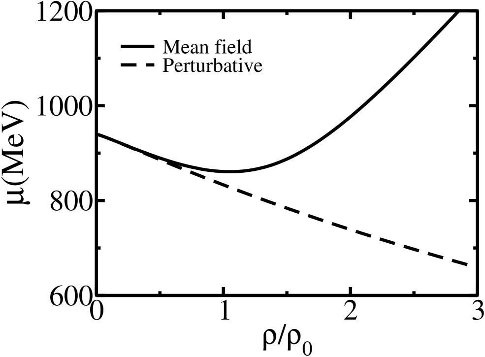
Figure 3: Chemical potential for direct contribution with $\sigma$ and $\omega$ meson exchange in symmetric nuclear matter. The dashed and solid curve represent the perturbative and MF results, respectively.

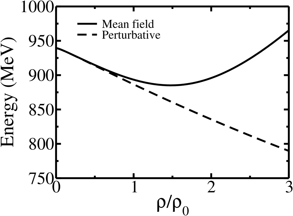
Figure 4: Total energy from direct contribution with $\sigma$ and $\omega$ meson exchange in symmetric nuclear matter. The dashed and solid curve represent the perturbative and MF results, respectively.

In Fig(3) we present the comparative study of the chemical potential obtained perturbatively and with MF calculation. At low density they tend to merge, while at higher density MF results differ significantly from the perturbative result. Numerically $\mu^{MFT}$ and $\mu^{per}$ are given by 861.07 MeV and 832.64 MeV respectively at normal matter density ($\rho_{0}=0.148{\rm fm^{-3}}$). For the numerical estimate we adopt the coupling parameter set as designated by ${\bf M0A}$ in ref.[23]. In Fig(4) we compare the results for total energy obtained from perturbative and MF calculation. This also shows at low density they tend to merge, while at higher density MF results become larger than the perturbative results. This is easily understood from Eq.(26) and (28). At saturation density numerical values are given by 886.43 MeV and 893.31 MeV for perturbative and MF calculation respectively.

Now we consider the exchange modification over the MF. Evaluating the exchange diagrams (Fig. 2), we obtain the interaction parameter as [27]

$$\left.\begin{array}[]{ll}f_{pp^{\prime}}^{ex,\sigma}&=-\frac{g_{\sigma}^{2}}{4\varepsilon_{p}^{0}\varepsilon_{p^{\prime}}^{0}}\frac{P.P^{\prime}+M^{*2}}{(P-P^{\prime})^{2}-m_{\sigma}^{2}}\\ f_{pp^{\prime}}^{ex,\omega}&=-\frac{g_{\omega}^{2}}{2\varepsilon_{p}^{0}\varepsilon_{p^{\prime}}^{0}}\frac{P.P^{\prime}-2M^{*2}}{(P-P^{\prime})^{2}-m_{\omega}^{2}}.\end{array}\right\}$$ (39)

With the help of Eq.(7), the LPs for scalar meson exchange reads as

$$f_{0}^{ex,\sigma} = \frac{g_{\sigma}^{2}}{8\varepsilon_{f}^{2}}\int_{-1}^{1}\frac{p_{f}^{2}(1-\cos\theta)+2M^{*2}}{2p_{f}^{2}(1-\cos\theta)+m_{\sigma}^{2}}{\rm d(\cos\theta)}$$ (40)

$$= \frac{g_{\sigma}^{2}}{8\varepsilon_{f}^{2}}\left[1-\left(\frac{m_{\sigma}^{2}-4M^{*2}}{4p_{f}^{2}}\right)\ln\left(1+\frac{4p_{f}^{2}}{m_{\sigma}^{2}}\right)\right],$$

and

$$\frac{1}{3}f_{1}^{ex,\sigma} = \frac{g_{\sigma}^{2}}{8\varepsilon_{f}^{2}}\int_{-1}^{1}\frac{p_{f}^{2}(1-\cos\theta)+2M^{*2}}{2p_{f}^{2}(1-\cos\theta)+m_{\sigma}^{2}}(\cos\theta){\rm d(\cos\theta)}$$ (41)

$$= \frac{g_{\sigma}^{2}}{8\varepsilon_{f}^{2}}\left[\left(\frac{m_{\sigma}^{2}-4M^{*2}}{2p_{f}^{2}}\right)\left\{1-\left(\frac{m_{\sigma}^{2}+2p_{f}^{2}}{4p_{f}^{2}}\right)\ln\left(1+\frac{4p_{f}^{2}}{m_{\sigma}^{2}}\right)\right\}\right].$$

Using Eqs.(40) and (41) we have

$$f_{0}^{ex,\sigma}-\frac{1}{3}f_{1}^{ex,\sigma} = \frac{g_{\sigma}^{2}}{8\varepsilon_{f}^{2}}\int_{-1}^{1}\frac{p_{f}^{2}(1-\cos\theta)+2M^{*2}}{2p_{f}^{2}(1-\cos\theta)+m_{\sigma}^{2}}(1-\cos\theta){\rm d(\cos\theta)}$$ (42)

$$= \frac{g_{\sigma}^{2}}{8\varepsilon_{f}^{2}}\left[1-\left(\frac{m_{\sigma}^{2}-4M^{*2}}{2p_{f}^{2}}\right)\left\{1-\frac{m_{\sigma}^{2}}{4p_{f}^{2}}\ln\left(1+\frac{4p_{f}^{2}}{m_{\sigma}^{2}}\right)\right\}\right].$$

It is this combination i.e. $f_{0}-\frac{1}{3}f_{1}$, which appears in the calculation of chemical potential and other relevant quantities. For massless scalar meson interaction, the above Eq.(42) turns out to be finite,

$$\left(f_{0}^{ex,\sigma}-\frac{1}{3}f_{1}^{ex,\sigma}\right)_{m_{\sigma}\rightarrow 0} = \frac{g_{\sigma}^{2}}{8p_{f}^{2}}\left(1+\frac{M^{*2}}{\varepsilon_{f}^{2}}\right).$$ (43)

Note that in the limit $m_{\sigma}\rightarrow 0$ both $f_{0}$ and $f_{1}$ are individually diverge because of the presence of $(1-\cos\theta)$ term in the denominator. In the massless limit such divergences are also contained in Eq.(40) and Eq.(41).

The dimensionless LPs $F_{0}$ and $F_{1}$ are defined as $F_{0}=N(0)f_{0}$ and $F_{1}=N(0)f_{1}$, where $N(0)$ is the density of states at the Fermi surface defined in Eq.(10).

$$F_{0}^{ex,\sigma} = g_{s}g_{I}\frac{g_{\sigma}^{2}p_{f}}{16\pi^{2}\varepsilon_{f}}\left[1-\left(\frac{m_{\sigma}^{2}-4M^{*2}}{4p_{f}^{2}}\right)\ln\left(1+\frac{4p_{f}^{2}}{m_{\sigma}^{2}}\right)\right],$$ (44)

and

$$\frac{1}{3}F_{1}^{ex,\sigma} = g_{s}g_{I}\frac{g_{\sigma}^{2}p_{f}}{16\pi^{2}\varepsilon_{f}}\left[\left(\frac{m_{\sigma}^{2}-4M^{*2}}{2p_{f}^{2}}\right)\left\{1-\left(\frac{m_{\sigma}^{2}+2p_{f}^{2}}{4p_{f}^{2}}\right)\ln\left(1+\frac{4p_{f}^{2}}{m_{\sigma}^{2}}\right)\right\}\right].$$ (45)

Similarly, for vector meson exchange we have

$$f_{0}^{ex,\omega} = \frac{g_{\omega}^{2}}{4\varepsilon_{f}^{2}}\int_{-1}^{1}\frac{p_{f}^{2}(1-\cos\theta)-M^{*2}}{2p_{f}^{2}(1-\cos\theta)+m_{\omega}^{2}}{\rm d(\cos\theta)}$$ (46)

$$= -\frac{g_{\omega}^{2}}{8\varepsilon_{f}^{2}}\left[-2+\frac{(m_{\omega}^{2}+2M^{*2})}{2p_{f}^{2}}\ln\left(1+\frac{4p_{f}^{2}}{m_{\omega}^{2}}\right)\right],$$

and

$$\frac{1}{3}f_{1}^{ex,\omega} = \frac{g_{\omega}^{2}}{4\varepsilon_{f}^{2}}\int_{-1}^{1}\frac{p_{f}^{2}(1-\cos\theta)-M^{*2}}{2p_{f}^{2}(1-\cos\theta)+m_{\omega}^{2}}(\cos\theta){\rm d(\cos\theta)}$$ (47)

$$= -\frac{g_{\omega}^{2}(m_{\omega}^{2}+2M^{*2})}{16\varepsilon_{f}^{2}p_{f}^{2}}\left[-2+\left(1+\frac{m_{\omega}^{2}}{2p_{f}^{2}}\right)\ln\left(1+\frac{4p_{f}^{2}}{m_{\omega}^{2}}\right)\right].$$

Using Eq.(46) and Eq.(47) we have

$$f_{0}^{ex,\omega}-\frac{1}{3}f_{1}^{ex,\omega} = \frac{g_{\omega}^{2}}{4\varepsilon_{f}^{2}}\int_{-1}^{1}\frac{p_{f}^{2}(1-\cos\theta)-M^{*2}}{2p_{f}^{2}(1-\cos\theta)+m_{\omega}^{2}}(1-\cos\theta){\rm d(\cos\theta)}$$ (48)

$$= \frac{g_{\omega}^{2}}{4\varepsilon_{f}^{2}}\left[1+\frac{(m_{\omega}^{2}+2M^{*2})}{4p_{f}^{2}}\left\{-2+\frac{m_{\omega}^{2}}{2p_{f}^{2}}\ln\left(1+\frac{4p_{f}^{2}}{m_{\omega}^{2}}\right)\right\}\right].$$

In the limit $m_{\omega}\rightarrow 0$ the above Eq.(48) turns into

$$\left(f_{0}^{ex,\omega}-\frac{1}{3}f_{1}^{ex,\omega}\right)_{m_{\omega}\rightarrow 0} = \frac{g_{\omega}^{2}}{4p_{f}^{2}}\left(1-\frac{2M^{*2}}{\varepsilon_{f}}\right).$$ (49)

This expression agrees with the previous calculation by Baym and Chin [27] who arrived at this result by direct evaluation of the integral by putting $m_{\omega}=0$ in Eq.(48). Here also to be noted, in the limit $m_{\omega}\rightarrow 0$ both $f_{0}$ and $f_{1}$ are individually divergent, but the combination $f_{0}-\frac{1}{3}f_{1}$ is finite as observed in the case of scalar ($\sigma$) meson exchange.

The dimensionless LPs for vector meson exchange reads:

$$F_{0}^{ex,\omega} = -g_{s}g_{I}\frac{g_{\omega}^{2}p_{f}}{16\pi^{2}\varepsilon_{f}}\left[-2+\frac{(m_{\omega}^{2}+2M^{*2})}{2p_{f}^{2}}\ln\left(1+\frac{4p_{f}^{2}}{m_{\omega}^{2}}\right)\right],$$ (50)

and

$$\frac{1}{3}F_{1}^{ex,\omega} = -g_{s}g_{I}\frac{g_{\omega}^{2}(m_{\omega}^{2}+2M^{*2})}{32\pi^{2}p_{f}\varepsilon_{f}}\left[-2+\left(1+\frac{m_{\omega}^{2}}{2p_{f}^{2}}\right)\ln\left(1+\frac{4p_{f}^{2}}{m_{\omega}^{2}}\right)\right].$$ (51)

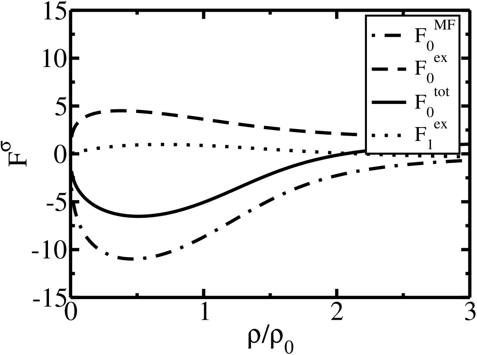
Figure 5: Dimensionless LPs in symmetric nuclear matter for $\sigma$ meson exchange in relativistic theory. $F_{0}^{MF}$, $F_{0}^{ex}$, $F_{0}^{tot}$ and $F_{1}^{ex}$ are denoted by dot-dashed, dashed, solid and dotted line respectively.

Table 1: Parameter sets used in this work.

Meson	Mass	Coupling
$\sigma$	$m_{\sigma}/M$=0.54	$g_{\sigma}/{4\pi}$=0.7936
$\omega$	$m_{\omega}/M$=0.8328	$g_{\omega}/{4\pi}$=0.9681

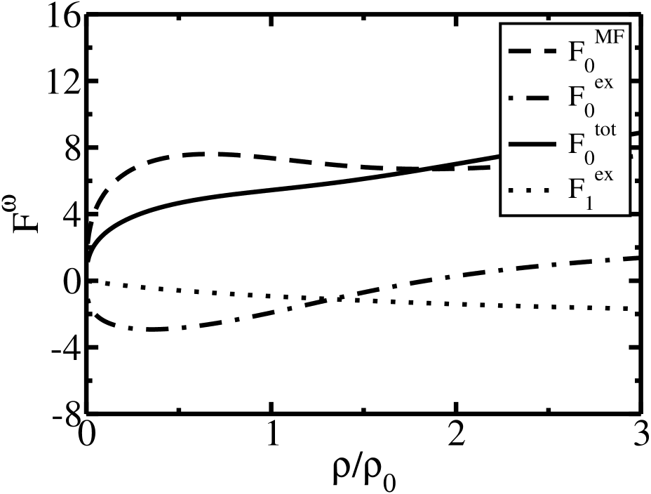
Figure 6: Dimensionless LPs for symmetric nuclear matter for $\omega$ meson exchange in relativistic theory. $F_{0}^{MF}$, $F_{0}^{ex}$, $F_{0}^{tot}$ and $F_{1}^{ex}$ are denoted by dashed, dot-dashed, solid and dotted line respectively.

Table 2: Dimensionless LPs for $\sigma$ and $\omega$ exchange at $\rho=\rho_{0}$.

Meson	$F_{0}^{MF}$	$F_{0}^{ex}$	$F_{0}^{tot}$	$F_{1}^{ex}$
$\sigma$	-8.65	3.61	-5.04	0.875
$\omega$	7.35	-1.91	5.44	-0.932

In Fig.(5) and Fig.(6) we present $F_{0}^{MF}$, $F_{0}^{ex}$, $F_{0}^{tot}$ and $F_{1}^{ex}$ as a function of baryon density for symmetric nuclear matter due to $\sigma$ and $\omega$ meson interaction respectively. It is to be noted, that $F_{0}^{MF}$ and $F_{0}^{ex}$ contribute in opposite sign for both $\sigma$ and $\omega$ meson exchange as it is seen from Table (2). We quote few numerical values of $F^{\sigma}$ and $F^{\omega}$ in Table (2) at normal matter density ($\rho_{0}=0.148{\rm fm^{-3}}$). It is to be noted that the numerical estimation of $F_{0}$ with MF in our case, differs from ref.[32]. This is due to different coupling parameters in these two models.

We now proceed to calculate chemical potential due to the exchange terms denoted by $\mu^{ex}$. As in ref.[27] we have

$$\frac{\partial\mu}{\partial\rho} = \frac{2\pi^{2}}{g_{s}g_{I}p_{f}^{2}}\left(\frac{\partial\varepsilon_{p}}{\partial p}\right)_{p=p_{f}}+f_{0}$$ (52)

$$= \frac{2\pi^{2}}{\mu g_{s}g_{I}p_{f}}-\frac{1}{3}f_{1}+f_{0},$$

and

$$\left(\frac{\partial\varepsilon_{p}}{\partial p}\right)_{p=p_{f}}=v_{f} = \frac{p_{f}}{\mu}-\frac{g_{s}g_{I}p_{f}^{2}}{2\pi^{2}}\frac{f_{1}}{3}.$$ (53)

Now from Eq.(52) one gets

$$\mu{\rm d\mu} = \left[p_{f}+g_{s}g_{I}\frac{\mu p_{f}^{2}}{2\pi^{2}}(f_{0}-\frac{1}{3}f_{1})\right]dp_{f}.$$ (54)

To calculate $\mu$, it is sufficient to let $\mu=\varepsilon_{f}$ in the right hand side of Eq.(54). With the constant of integration adjusted so that at high density $p_{f}\simeq\varepsilon_{f}$, Eq.(54) upon integration together with Eq.(42) yield

$$\mu^{ex}_{\sigma} = \varepsilon_{f}+\frac{g_{s}g_{I}g_{\sigma}^{2}}{128\pi^{2}\varepsilon_{f}}M^{*2}\left[-2y_{\sigma}(4-y_{\sigma}^{2})^{3/2}\tan^{-1}\left(\frac{x\sqrt{4-y_{\sigma}^{2}}}{y_{\sigma}\sqrt{1+x^{2}}}\right)\right.$$ (55)

$$\left.~{}~{}~{}~{}~{}~{}~{}~{}~{}~{}~{}~{}~{}~{}~{}~{}~{}~{}~{}~{}~{}~{}~{}~{}~{}~{}~{}+\frac{y_{\sigma}^{2}(4-y_{\sigma}^{2})\sqrt{1+x^{2}}}{x}\ln\left(1+\frac{4x^{2}}{y_{\sigma}^{2}}\right)+4x\sqrt{1+x^{2}}\right.$$

$$\left.~{}~{}~{}~{}~{}~{}~{}~{}~{}~{}~{}~{}~{}~{}~{}~{}~{}~{}~{}~{}~{}~{}~{}~{}~{}+2(y_{\sigma}^{4}-6y_{\sigma}^{2}+6)\ln(x+\sqrt{1+x^{2}})\right],$$

where $x=p_{f}/M^{*}$ and $y_{\sigma}=m_{\sigma}/M^{*}$.

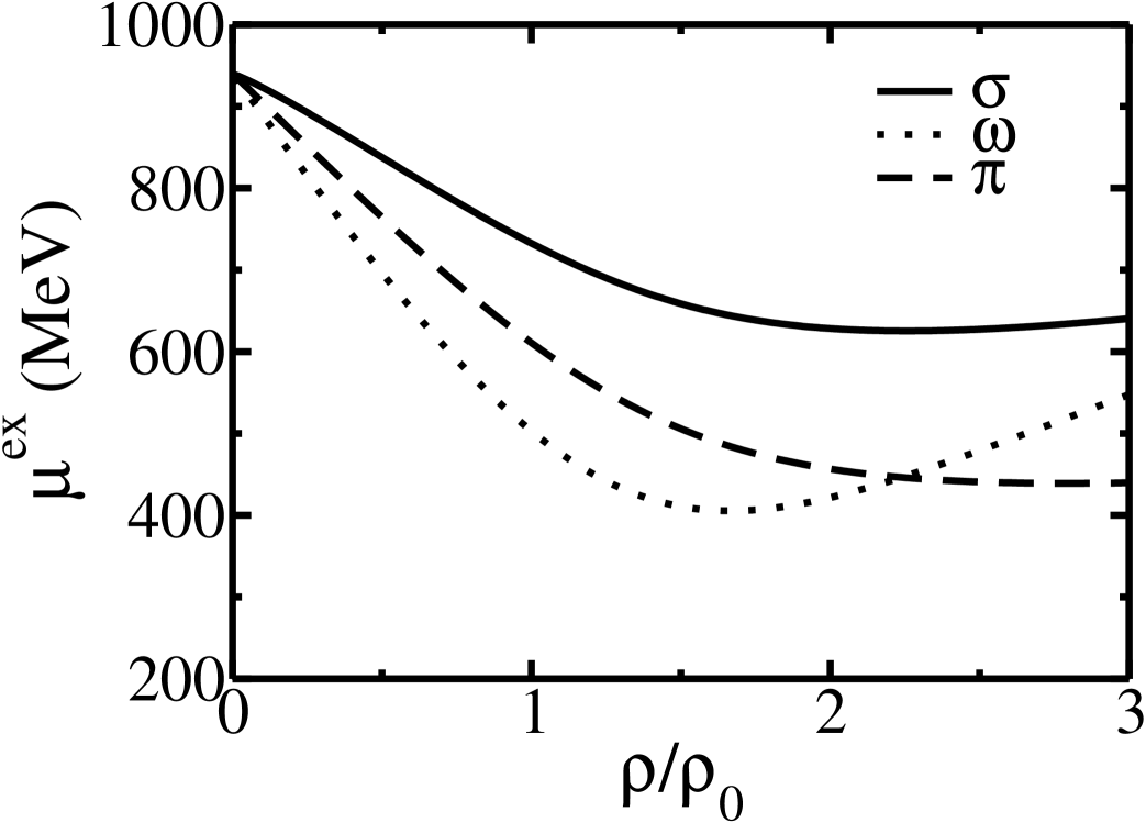
Figure 7: Density dependent of exchange chemical potential in symmetric nuclear matter. $\sigma$,$\omega$ and $\pi$ mesons are denoted by solid, dotted and dashed line respectively.

For massless meson limit i.e. at $m_{\sigma}\rightarrow 0$ implies $y_{\sigma}\rightarrow 0$ we have

$$\mu^{ex}_{\sigma}\left|\right._{m_{\sigma}\rightarrow 0} = \varepsilon_{f}+g_{s}g_{I}\frac{g_{\sigma}^{2}M^{*2}}{32\pi^{2}\varepsilon_{f}}\left[x\sqrt{1+x^{2}}+3\ln(x+\sqrt{1+x^{2}})\right].$$ (56)

Similarly for vector meson interaction, using Eq.(48) and Eq.(54) one obtains

$$\mu_{\omega}^{ex} = \varepsilon_{f}-\frac{g_{s}g_{I}g_{\omega}^{2}M^{*2}}{64\pi^{2}\varepsilon_{f}}\left[\frac{2y_{\omega}(y_{\omega}^{4}-2y_{\omega}^{2}-8)}{\sqrt{-y_{\omega}^{2}+4}}\tan^{-1}\left(\frac{x\sqrt{-y_{\omega}^{2}+4}}{y_{\omega}\sqrt{1+x^{2}}}\right)\right.$$ (57)

$$\left.~{}~{}~{}~{}~{}~{}~{}~{}~{}~{}~{}~{}~{}~{}~{}~{}~{}~{}~{}~{}~{}~{}~{}+\frac{y_{\omega}^{2}(y_{\omega}^{2}+2)\sqrt{1+x^{2}}}{x}\ln\left(1+\frac{4x^{2}}{y_{\omega}^{2}}\right)-4x\sqrt{1+x^{2}}\right.$$

$$\left.~{}~{}~{}~{}~{}~{}~{}~{}~{}~{}~{}~{}~{}~{}~{}~{}~{}~{}~{}~{}~{}~{}~{}~{}+2(6-y_{\omega}^{4})\ln(x+\sqrt{1+x^{2}})\right].$$

Here $y_{\omega}=m_{\omega}/M^{*}$. For massless limit of vector meson the expression for chemical potential reads as

$$\mu^{ex}_{\omega} = \varepsilon_{f}+g_{s}g_{I}\frac{g_{\omega}^{2}M^{*2}}{16\pi^{2}\varepsilon_{f}}\left[x\sqrt{1+x^{2}}-3\ln(x+\sqrt{1+x^{2}})\right].$$ (58)

In low density limit ($M^{*}\rightarrow M$) for the massless meson exchange we reproduce the expression derived earlier [27, 12].

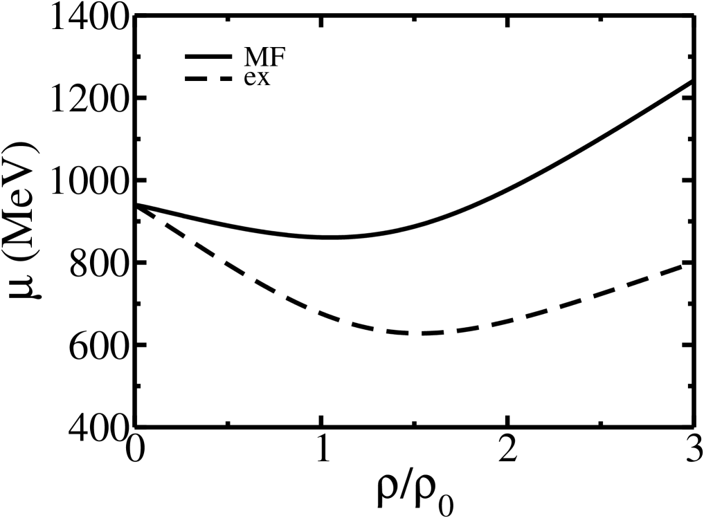
Figure 8: Comparison of mean field and exchange results of chemical potential in symmetric nuclear matter. Direct contributions are plotted by solid curve and exchange contributions by dashed curve.

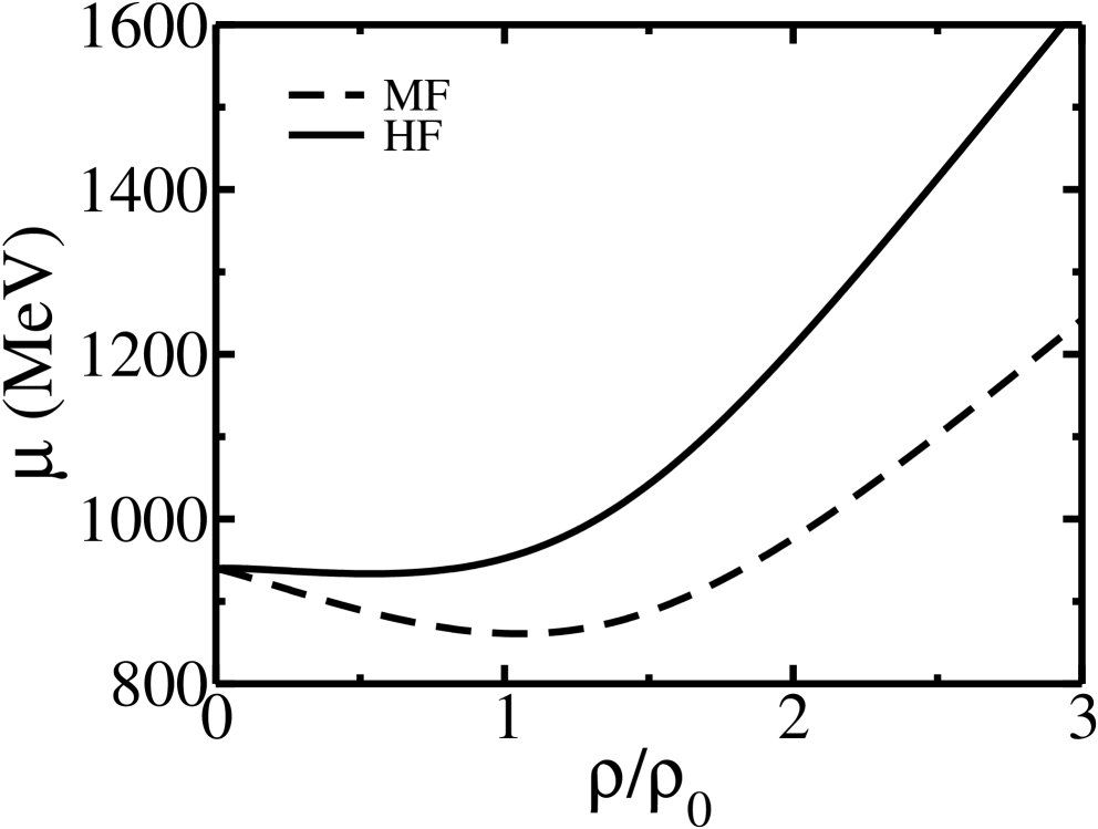
Figure 9: Comparison of chemical potential with MFT and HF case in symmetric nuclear matter. MF and HF results denoted by dashed and solid line respectively.

Once the $\mu^{ex}$ is determined, one can readily calculate its contribution to the energy density. For scalar meson interaction it is given by [27, 12],

$$E^{ex}_{\sigma} = \frac{1}{2}\int{\rm d\rho}(\mu^{ex}_{\sigma}-\varepsilon_{f})$$ (59)

$$= g_{s}^{2}g_{I}^{2}\frac{g_{\sigma}^{2}M^{*4}}{512\pi^{4}}\left[y_{\sigma}^{2}(4-y_{\sigma}^{2})\left\{-\frac{x^{2}}{2}+\frac{y_{\sigma}^{2}+4x^{2}}{8}\ln\left(1+\frac{4x^{2}}{y_{\sigma}^{2}}\right)\right\}+x^{4}\right.$$

$$\left.~{}~{}~{}~{}~{}~{}~{}~{}~{}~{}~{}~{}~{}~{}~{}~{}~{}-\frac{1}{2}(y_{\sigma}^{4}-6y_{\sigma}^{2}+6)(\{x\sqrt{1+x^{2}}-\ln(x+\sqrt{1+x^{2}})\}^{2}-x^{4})+I_{\sigma}\right],$$

where

$$I_{\sigma} = -2y_{\sigma}(4-y_{\sigma}^{2})^{3/2}\int\frac{x^{2}}{\sqrt{1+x^{2}}}\tan^{-1}\left(\frac{x\sqrt{4-y_{\sigma}^{2}}}{y_{\sigma}\sqrt{1+x^{2}}}\right){\rm d}x.$$ (60)

Similarly, for vector meson exchange we obtain

$$E^{ex}_{\omega} = \frac{1}{2}\int{\rm d\rho}(\mu^{ex}_{\omega}-\varepsilon_{f})$$ (61)

$$= -g_{s}^{2}g_{I}^{2}\frac{g_{\omega}^{2}M^{*4}}{256\pi^{4}}\left[y_{\omega}^{2}(2+y_{\omega}^{2})\left\{-\frac{x^{2}}{2}+\frac{y_{\omega}^{2}+4x^{2}}{8}\ln\left(1+\frac{4x^{2}}{y_{\omega}^{2}}\right)\right\}-x^{4}\right.$$

$$\left.~{}~{}~{}~{}~{}~{}~{}~{}~{}~{}~{}~{}~{}~{}~{}~{}~{}+\left(\frac{y_{\omega}^{4}}{2}-3\right)\left(\{x\sqrt{1+x^{2}}-\ln(x+\sqrt{1+x^{2}})\}^{2}-x^{4}\right)+I_{\omega}\right],$$

where

$$I_{\omega} = \frac{2y_{\omega}(y_{\omega}^{4}-2y_{\omega}^{2}-8)}{\sqrt{4-y_{\omega}^{2}}}\int\frac{x^{2}}{\sqrt{1+x^{2}}}\tan^{-1}\left(\frac{x\sqrt{4-y_{\omega}^{2}}}{y_{\omega}\sqrt{1+x^{2}}}\right){\rm d}x.$$ (62)

Thus for the case of massless mesons [27, 12], we have

$$E^{ex}_{\sigma}|_{m_{\sigma}\rightarrow 0} = \frac{g_{\sigma}^{2}M^{*4}}{8\pi^{4}}[x^{4}-\frac{3}{4}\{x\sqrt{1+x^{2}}-\ln(x+\sqrt{1+x^{2}})\}^{2}],$$ (63)

and

$$E^{ex}_{\omega}|_{m_{\omega}\rightarrow 0} = -\frac{g_{\omega}^{2}M^{*4}}{8\pi^{4}}[x^{4}-\frac{3}{2}\{x\sqrt{1+x^{2}}-\ln(x+\sqrt{1+x^{2}})\}^{2}].$$ (64)

Due to presence of pion fields in the chiral Lagrangian we have component in the interaction which acts on the isospin fluctuation. One can derive the quasiparticle interaction with isospin dependency by the same procedure as for $\sigma$ and $\omega$ meson. Pion, being a pseudoscalar, fails to contribute at the MF level forcing us to go beyond MFT so as to include pionic contribution to the FLPs. It is to be noted that, in exchange diagram pion have both isoscalar and isovector contribution to FLPs. Detailed calculation for isoscalar contribution to FLPs is similar as $\sigma$ and $\omega$ meson. For brevity, we present only dimensionless FLPs and their contribution to energy density. We also quote their numerical values.

The dimensionless LPs due to $\pi$ exchange are

$$F^{ex,\pi}_{0}=-g_{s}g_{I}\frac{3g_{A}^{2}p_{f}M^{*2}}{64\pi^{2}f_{\pi}^{2}\varepsilon_{f}}\left[-2+\frac{m_{\pi}^{2}}{2p_{f}^{2}}\ln\left(1+\frac{4p_{f}^{2}}{m_{\pi}^{2}}\right)\right],$$ (65)

and

$$\frac{1}{3}F^{ex,\pi}_{1}=-g_{s}g_{I}\frac{3g_{A}^{2}m_{\pi}^{2}M^{*2}}{128\pi^{2}f_{\pi}^{2}p_{f}\varepsilon_{f}}\left[-2+\left(\frac{m_{\pi}^{2}}{2p_{f}^{2}}+1\right)\ln\left(1+\frac{4p_{f}^{2}}{m_{\pi}^{2}}\right)\right].$$ (66)

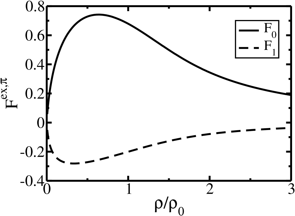
Figure 10: Dimensionless LPs in symmetric nuclear matter for pion exchange in relativistic theory. Solid and dashed line represent $F_{0}^{\pi}$ and $F_{1}^{\pi}$ respectively.

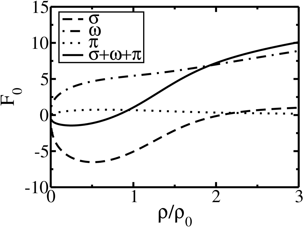
Figure 11: Dimensionless relativistic LP $F_{0}$ in symmetric nuclear matter. $\sigma$, $\omega$, $\pi$ and total contribution are denoted by dashed, dot-dashed, dotted and solid line respectively.

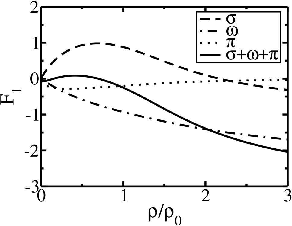
Figure 12: Dimensionless relativistic LP $F_{1}$ in symmetric nuclear matter. $\sigma$, $\omega$, $\pi$ and total contribution are denoted by dashed, dot-dashed, dotted and solid line respectively.

In the non-relativistic limit $\varepsilon_{f}\rightarrow M^{*}$, one obtains the same expression of $F_{1}^{\pi}$ as reported in [4, 35]. In Fig.(10) we show the density dependence of $F_{0}$ and $F_{1}$ due to pionic interaction. Numerically at nuclear saturation density $(\rho_{0}=0.148{\rm fm^{-3}})$, $F^{ex,\pi}_{0}=0.68$ and $F^{ex,\pi}_{1}=-0.2$.

In Fig.(11) and Fig.(12) we plot separate and total contribution of $F_{0}$ and $F_{1}$ due to $\sigma$, $\omega$ and $\pi$ exchange respectively. Interestingly, individual contribution to LPs of $\sigma$ and $\omega$ meson are large while sum of their contribution to $F_{0}^{tot}$ is small due to the sensitive cancellation of $F_{0}^{\sigma}$ and $F_{0}^{\omega}$ as can be seen from Fig.(11). Such a cancellation is responsible for the nuclear saturation dynamics [33, 34]. Numerically, $F_{0}^{\sigma+\omega}$ is approximately $3/2$ times smaller than $F_{0}^{\pi}$ as can be seen from Table (3).

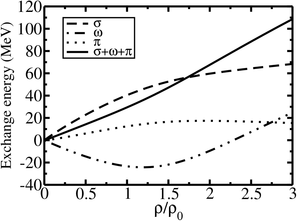
Figure 13: Comparison of separate and total exchange energy obtained from FLT in symmetric nuclear matter.$\sigma$, $\omega$, $\pi$ and total contribution are denoted by dashed, dot-dashed, dotted and solid line respectively.

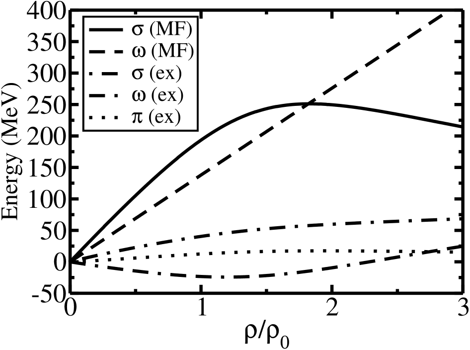
Figure 14: Comparison of mean field energy and exchange energy obtained from FLT in symmetric nuclear matter. $E_{\sigma}^{MF}$, $E_{\omega}^{MF}$, $E_{\sigma}^{ex}$, $E_{\omega}^{ex}$ and $E_{\pi}^{ex}$ are denoted by solid, dashed, dot-dashed, dash-dashed and dotted line respectively.

The exchange energy density is given by

$$E^{ex}_{\pi} = -g_{s}^{2}\frac{3g_{A}^{2}M^{*6}}{128f_{\pi}^{2}\pi^{4}}\left[I_{\pi}+y_{\pi}^{4}\left\{-\frac{x^{2}}{2}+\frac{y_{\pi}^{2}+4x^{2}}{8}\ln\left(1+\frac{4x^{2}}{y_{\pi}^{2}}\right)\right\}-x^{4}\right.$$ (67)

$$\left.+\left(\frac{y_{\pi}^{4}}{2}-y_{\pi}^{2}-1\right)\left(\{x\eta-\ln(x+\eta)\}^{2}-x^{4}\right)\right],$$

where $y_{\pi}=m_{\pi}/M^{*}$ and

$$I_{\pi}=-2y_{\pi}^{3}\sqrt{4-y_{\pi}^{2}}\int\frac{x^{2}}{\eta}\tan^{-1}\left(\frac{x\sqrt{4-y_{\pi}^{2}}}{y_{\pi}\eta}\right){\rm d}x.$$ (68)

For the massless pion this reads as

$$E^{ex}_{\pi}{\Big{|}}_{m_{\pi}\rightarrow 0} = \frac{3g_{A}^{2}M^{*6}}{32f_{\pi}^{2}\pi^{4}}[x\eta-\ln(x+\eta)]^{2}.$$ (69)

In Fig.(13) and Fig.(14) we show the density dependence of energy due $\sigma$, $\omega$ and $\pi$ meson exchanges. Numerical values are quoted in Table(5).

It might be mentioned here that in the massless meson limit, Eq.(63), (64) and (69) can be evaluated analytically from two loop ring diagrams of ref.[23] using Eqs.(54), (55) and (56). We have checked and the expression for the energies are found to be consistent with each other. With massive meson results are compared numerically. Numerical estimation of exchange energy from loop diagram and RFLT are found to be few percent limit.

Table 3: Dimensionless Landau parameters and chemical potential at $\rho=\rho_{0}$. Note that, $F_{0}$, $F_{1}$ are the dimensionless isoscalar LPs.

Meson	$F_{0}$	$F_{1}$	$\mu^{ex}(MeV)$
$\sigma$	-5.04	0.875	731.89
$\omega$	5.44	-0.93	501.82
$\pi$	0.68	-0.20	609.88

Table 4: Chemical potential in MeV from FLT at $\rho=\rho_{0}$.

Meson	$\mu^{ex}$	$\mu^{MF}$	$\mu^{HF}$
$\sigma$	731.89	-	-
$\omega$	501.82	-	-
$\pi$	609.88	-	-
$\sigma+\omega+\pi$	675.63	861.07	952.73

Finally we reproduce saturation property of nuclear matter i.e. $E/{\rho}-M=-16.12$ MeV at $p_{f}=1.3{\rm fm^{-1}}$ with those energy calculated from RFLPs.

Table 5: MF and Exchange energy in MeV from FLT at $\rho=\rho_{0}$.

Meson	$E^{MF}$	$E^{ex}$
$\sigma$	193.86	40.48
$\omega$	138.39	-23.41
$\pi$	-	12.49

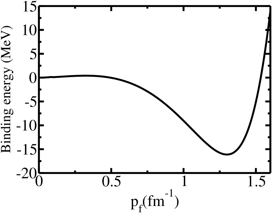
Figure 15: Binding energy graph from FLT for symmetric nuclear matter.

III.3 Incompressibility and First Sound Velocity

In nuclear matter several important relationships exist between nuclear observables and the FLPs. The thermodynamical parameters can be expressed in terms of few LPs. For example we present the incompressibility ($K$) and first sound velocity ($c_{1}$)[7, 32].

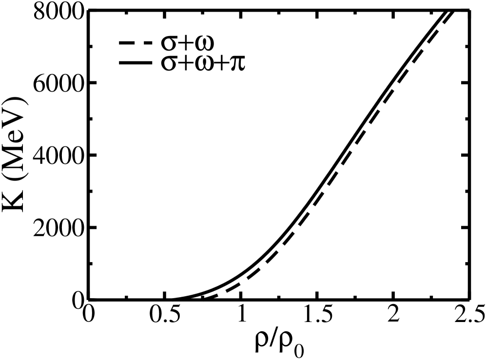
Figure 16: Compressibility $K$ in symmetric nuclear matter.

Incompressibility of the Fermi liquid may be derived as in the non-relativistic theory by the second derivative of energy density ($E$) with respect to the number density $\rho$ [7, 32];

$$K \equiv \rho\frac{\partial^{2}E}{\partial\rho^{2}}$$ (70)

$$= \rho\frac{\partial\mu}{\partial\rho}.$$

If energy density $E$ is given in terms of number density $\rho$, then the expression for incompressibility or compression modulus in terms of LPs is given by,

$$K = \frac{3p_{f}^{2}}{\varepsilon_{f}}(1+F_{0}).$$ (71)

Now consider the effect of quasiparticle collision on the collective modes of a neutral Fermi liquid. Suppose the frequency of the mode is $\omega$, while the quasiparticle collision frequency is $\nu$. For the limit $\omega<<\nu$, many quasiparticle collision takes place during time interval $\omega^{-1}$. Then the region is collision-dominated, or hydrodynamic regime [32]. Under this circumstances, organized density fluctuation is possible and hydrodynamic or first sound waves are generated. Hydrodynamic sound propagates only when the system attains the local thermodynamic equilibrium in a time much shorter than the time interval of the sound oscillation.

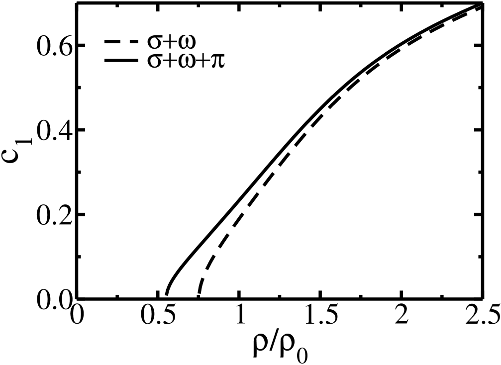
Figure 17: First sound velocity $c_{1}$ in symmetric nuclear matter.

The first sound velocity is given by [27]

$$c_{1}^{2}~{}=~{}\frac{\partial P}{\partial E} = \frac{\partial P}{\partial\mu}\frac{\partial\mu}{\partial\rho}\frac{\partial\rho}{\partial E}$$ (72)

$$= \frac{\rho}{\mu}\frac{\partial\mu}{\partial\rho},$$

With the help of Eq.(52), Eq.(72) yields

$$c_{1}^{2} = \frac{1}{3}\frac{p_{f}^{2}}{\mu^{2}}\frac{1+F_{0}}{1+\frac{1}{3}F_{1}}$$ (73)

$$= \frac{1}{3}\frac{p_{f}^{2}}{\mu^{2}}\left[1+\frac{g_{s}g_{I}\mu p_{f}}{2\pi^{2}}(f_{0}-\frac{1}{3}f_{1})\right].$$

Corresponding values of the incompressibility and the first sound velocity are plotted in Fig.(16) and Fig.(17) separately with $\sigma+\omega$ and $\sigma+\omega+\pi$ contribution. It is observed that for combined $\sigma$ and $\omega$ meson at $\rho<0.75\rho_{0}$, $F_{0}<-1$ and the resulting compressibility turns out to be negative. While for $\pi$ meson together with $\sigma$ and $\omega$ meson the same conclusion can be drawn at $\rho<0.55\rho_{0}$ . This is the region where the attractive interaction due to the exchange of scalar mesons overwhelms the repulsive force coming from vector meson exchange, and consequently the system becomes unstable [32]. On the other hand, as the density increases, the attractive scalar meson exchange force tends to be suppressed by the relativistic effect and the net quasiparticle interaction become repulsive. At nuclear saturation density ($\rho_{0}=0.148{\rm fm^{-3}}$) we have $K=476.04$ MeV and $705.84$ MeV for combined $\sigma+\omega$ and $\sigma+\omega+\pi$ mesons respectively. The small effective mass is responsible for large incompressibility. The first sound velocity $c_{1}=0.19$ for $\sigma+\omega$ and $0.23$ for $\sigma+\omega+\pi$ at normal nuclear matter density and at all densities $c_{1}$ is smaller than the velocity of light, which is consistent with causality [32].

IV Isovector Landau parameter and symmetry energy

In this section we proceed to calculate isovector LPs due to pion exchange. The isovector contribution to interaction parameter is

$$f_{pp^{\prime}}^{\prime}{\Big{|}}_{p\simeq p^{\prime}=p_{f}} = -\frac{1}{2}\frac{g_{A}^{2}M^{*2}}{4f_{\pi}^{2}\varepsilon_{f}^{2}}\left\{\frac{p_{f}^{2}(1-\cos\theta)}{2p_{f}^{2}(1-\cos\theta)+m_{\pi}^{2}}\right\}.$$ (74)

where $g_{A}^{2}=1.5876$ , $f_{\pi}=93MeV$ and $m_{\pi}=139$ MeV [23]. Here $-1/2$ is isospin factor in isovector channel [5].

Using Eq.(7) and (74) we derive isovector LPs $f^{\prime}_{0}$ and $f^{\prime}_{1}$,

$$f^{\prime}_{0} = -\frac{g_{A}^{2}M^{*2}p_{f}^{2}}{16f_{\pi}^{2}\varepsilon_{f}^{2}}\int_{-1}^{1}\frac{(1-\cos\theta)}{2p_{f}^{2}(1-\cos\theta)+m_{\pi}^{2}}{\rm d(\cos\theta)}$$ (75)

$$= \frac{g_{A}^{2}M^{*2}}{32f_{\pi}^{2}\varepsilon_{f}^{2}}\left[-2+\frac{m_{\pi}^{2}}{2p_{f}^{2}}\ln\left(1+\frac{4p_{f}^{2}}{m_{\pi}^{2}}\right)\right],$$

and

$$\frac{1}{3}f^{\prime}_{1} = -\frac{g_{A}^{2}M^{*2}p_{f}^{2}}{16f_{\pi}^{2}\varepsilon_{f}^{2}}\int_{-1}^{1}\frac{\cos\theta(1-\cos\theta)}{2p_{f}^{2}(1-\cos\theta)+m_{\pi}^{2}}{\rm d(\cos\theta)}$$ (76)

$$= \frac{g_{A}^{2}M^{*2}m_{\pi}^{2}}{64f_{\pi}^{2}\varepsilon_{f}^{2}p_{f}^{2}}\left[-2+\left(\frac{m_{\pi}^{2}}{2p_{f}^{2}}+1\right)\ln\left(1+\frac{4p_{f}^{2}}{m_{\pi}^{2}}\right)\right].$$

The dimensionless LPs $F_{0}^{\prime}=N(0)f_{0}^{\prime}$ and $F_{1}^{\prime}=N(0)f_{1}^{\prime}$ are given below. Here, $N(0)$ is the density of states at the Fermi surface defined in Eq.(10).

$$F^{\prime}_{0} = g_{s}g_{I}\frac{g_{A}^{2}p_{f}M^{*2}}{64\pi^{2}f_{\pi}^{2}\varepsilon_{f}}\left[-2+\frac{m_{\pi}^{2}}{2p_{f}^{2}}\ln\left(1+\frac{4p_{f}^{2}}{m_{\pi}^{2}}\right)\right],$$ (77)

and

$$\frac{1}{3}F^{\prime}_{1} = g_{s}g_{I}\frac{g_{A}^{2}m_{\pi}^{2}M^{*2}}{128\pi^{2}f_{\pi}^{2}p_{f}\varepsilon_{f}}\left[-2+\left(\frac{m_{\pi}^{2}}{2p_{f}^{2}}+1\right)\ln\left(1+\frac{4p_{f}^{2}}{m_{\pi}^{2}}\right)\right].$$ (78)

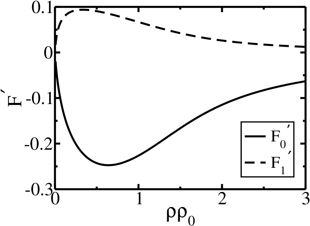
Figure 18: Density dependent of isovector LPs in symmetric nuclear matter.

Knowing the isovector LPs, to which here only the pion contributes, one can calculate nuclear symmetry energy. The symmetry energy is defined as the difference of energy between the neutron matter and symmetric nuclear matter which we denote as $\beta$ [32].

Analytically, the symmetry energy is defined from the expansion of the energy per nucleon $E^{\prime}(\rho,\alpha)$ in terms of the asymmetry parameter $\alpha$ defined as [36]

$$\alpha\equiv-\frac{\rho_{3}}{\rho}=\frac{\rho_{n}-\rho_{p}}{\rho}=\frac{N-Z}{A}.$$ (79)

We have

$$E^{\prime}(\rho,\alpha)\equiv\frac{E(\rho,\alpha)}{\rho}=E^{\prime}(\rho)+E^{\prime}_{sym}(\rho)\alpha^{2}+{\cal{O}}(\alpha^{4})+.....$$ (80)

and so, in general,

$$E^{\prime}_{sym}\equiv\beta = \frac{1}{2}\frac{\partial^{2}E^{\prime}(\rho,\alpha)}{\partial\alpha^{2}}{\Big{|}}_{\alpha=0}$$ (81)

$$= \frac{1}{2}\rho\frac{\partial^{2}E}{\partial\rho_{3}^{2}}{\Big{|}}_{\rho_{3}=0}.$$

In terms of LPs, the symmetry energy can be expressed as

$$\beta=\frac{p_{f}^{2}}{6\varepsilon_{f}}(1+F^{\prime}_{0}),$$ (82)

where $F^{\prime}_{0}$ is the isospin dependent LP. Numerically at saturation density $(\rho=\rho_{0})$ we obtain $\beta=14.57$ MeV. So relatively small contribution to $\beta$ comes from one-pion exchange diagram [37].

Similar to the hydrodynamic sound corresponding to the total baryon density oscillation, we consider hydrodynamic isospin sound which accompany the out-of-phase oscillations of proton and neutron density. Isospin sound velocity $c_{1}^{\prime}$ is given by [32]

$$c_{1}^{\prime} = v_{f}\sqrt{\frac{\varepsilon_{f}}{3\mu}(1+F_{0}^{\prime})}$$ (83)

Numerically at saturation density $(\rho=\rho_{0})$ we obtain $c_{1}^{\prime}=0.17$.

V Discussion

In this work we determine the RFLPs using effective chiral model to study the properties of DNM. We compare the MF results with the corresponding perturbative results for the FLPs. It is seen at low densities, they converge but perturbative results differs significantly with the mean field results at higher density.

We have estimated the pionic contribution to the FLPs which can contribute only in exchange diagrams. It is seen that numerically pionic contribution is smaller than the corresponding $\sigma$ and $\omega$ meson results, however, we show this is still important in various physical quantities as $\sigma$ and $\omega$ meson contribute in opposite sign and pionic contribution is comparable to the sum of the contributions coming from the scalar and vector meson exchanges. Among the other physical quantities we also evaluate the sound velocity and incompressibility and symmetry energy etc. The results for the sound velocities gives the correct causal limit at extremely high densities. It is also shown that, the system is stable with respect to density fluctuation at and above the nuclear saturation density and exhibit instability in relatively low density regimes.

Here we also have calculated exchange energy densities by using FLPs calculated relativistically. The results are found to be consistent with what are obtains by directly evaluating the nucleon loops [23], this gives further support to the present approach.

Acknowledgments

The authors would like to thank G.Baym and C.Gale for their valuable comments. We also wish to thank P.Roy for his critical reading of the manuscript.

References

- [1] S.A.Chin, Phys.Lett.B62, 263 (1976).
- [2] J.Speth, V.Klemt, J.Wambach and G.E.Brown Nucl.Phys.A343, 382 (1980).
- [3] C.J.Horowitz and B.D.Serot, Nucl.Phys.A399, 529 (1983).
- [4] B.Friman and M.Rho, Nucl.Phys.A606, 303-319 (1996).
- [5] B.Friman, M.Rho, C.Song, Phys.Rev.C59, 3357-3370 (1999).
- [6] C.Song, Phys.Rept.347, 289 (2001).
- [7] J.W.Holt, G.E.Brown, J.D.Holt and T.T.S.Kuo, Nucl.Phys.A785, 322 (2007).
- [8] B.D.Serot, Rept.Prog.Phys.55, 1855-1946 (1992).
- [9] J.D.Walecka, Annals of Physics 83, 491 (1974).
- [10] B.D.Serot and J.D.Walecka, The Relativistic Nuclear Many Body Problem, Advances in Nuclear Physics, Vol.16, editted by J.W.Negele and E.Vogt (Plenum, New York, 1986).
- [11] S.A.Chin and J.D.Walecka, Phys.Lett.B52, 24 (1974).
- [12] S.A.Chin, Annals of Physics 108, 301 (1977).
- [13] B.D.Serot, Phys.Lett.B86, 146 (1979); Erratum, Phys.Lett B87, 403 (1979).
- [14] J.I.Kapusta, Phys.Rev.C23, 1648 (1981).
- [15] T.Matsui and B.D.Serot, Annals of Physics 144, 107-167 (1982).
- [16] R.J.Furnstahl, C.E.Price and G.E.walker, Phys.Rev.C36, 2590 (1987).
- [17] R.J.Furnstahl and B.D.Serot, Phys.Lett.B316, 12 (1993).
- [18] R.J.Furnstahl, H.B.Tang and B.D.Serot, Phys.Rev.C52, 1368 (1995).
- [19] R.J.Furnstahl, B.D.Serot and H.B.Tang, Nucl.Phys. A598, 539 (1996).
- [20] R.J.Furnstahl, R.J.Perry, B.D.Serot, Phys.Rev.C40, 321 (1989).
-
[21]
R.J.Furnstahl, B.D.Serot and H.B.Tang,
Nucl.Phys.A615, 441 (1997),
- [22] B.D.Serot and J.D.Walecka, Int.J.Mod.Phys.E6, 515 (1997). Erratum, Nucl.Phys.A640, 505 (1998).
- [23] Y.Hu, J.McIntire, B.D.Serot, Nucl.Phys.A794, 187 (2007).
- [24] S.Biswas and A.K.Dutt-Mazumder, Phys.Rev.C77, 045201 (2008).
- [25] D.Pines and P.Noziéres, The Theory Of Quantum Liquids, United States of America (1966).
- [26] G.baym and C.Pethick, Landau Fermi liquid Theory: Concepts and Applications, United States Of America (1991).
- [27] G.Baym and S.A.Chin, Nucl.Phys.A262, 527 (1976).
- [28] A.B.Migdal, Rev.Mod.Phys.50, 107 (1978).
-
[29]
A.B.Migdal, Theory of Finite Fermi Systems (1967)
(Wiley, New York) (Russ.ed.1965),
A.B.Migdal, Nuclear Theory: The Quasiparticle Method, (Benjamin, New York) (1968). - [30] S.Krewald, K.Nakayama and J.Speth, Phys.Rept. 161, 103-170 (1988) .
- [31] G.E.Brown, Rev.Mod.Phys.43, 1 (1971).
- [32] T.Matsui, Nucl.Phys.A370, 365 (1981).
- [33] L.S.Celenza and C.M.Shakin, Relativistic Nuclear Physics, (World Scientific, USA) (1986).
- [34] M.R.Anastasio, L.S.Celenza, W.S.Pong and C.M.Shakin, Phys.Rept.100, 327-392 (1983).
- [35] G.E.Brown and M.Rho, Nucl.Phys.A338, 269 (1980).
- [36] V.Greco, M.colonna, M.Di Toro and F.Matera, Phys.Rev.C67, 015203 (2003).
- [37] A.E.L.Dieperink, Y.Dewulf, D.Van Neck, M.Waroquier and V.Rodin, Phys.Rev.C68, 064307 (2003).