Diagnosing space telescope misalignment and jitter using stellar images

Abstract

Accurate knowledge of the telescope’s point spread function (PSF) is essential for the weak gravitational lensing measurements that hold great promise for cosmological constraints. For space telescopes, the PSF may vary with time due to thermal drifts in the telescope structure, and/or due to jitter in the spacecraft pointing (ground-based telescopes have additional sources of variation). We describe and simulate a procedure for using the images of the stars in each exposure to determine the misalignment and jitter parameters, and reconstruct the PSF at any point in that exposure’s field of view. The simulation uses the design of the SNAP telescope. Stellar-image data in a typical exposure determines secondary-mirror positions as precisely as $20\,{\rm nm}$. The PSF ellipticities and size, which are the quantities of interest for weak lensing are determined to $4.0\times 10^{-4}$ and $2.2\times 10^{-4}$ accuracies respectively in each exposure, sufficient to meet weak-lensing requirements. We show that, for the case of a space telescope, the PSF estimation errors scale inversely with the square root of the total number of photons collected from all the usable stars in the exposure.

1 Introduction

The accelerated expansion of the universe is one of the most puzzling astrophysical discovery of the century. The proposed explanations are dark energy, modified gravity and feedback from density fluctuations. To explore the mystery, a few large astronomical surveys are underway (DES, ACT, SPT) or in planning stages (SNAP, DESTINY, LSST, EUCLID). The sensitivity of these surveys to the expansion of the universe comes from both cosmological distances and growth of density perturbations as a function of the cosmic time or redshift. The probes utilized are Type-Ia supernova, weak gravitational lensing (WL), baryon acoustic oscillations, galaxy cluster counting (selected by optical or using Sunyave-Zeldovic effect), and the integrated Sachs-Wolfe effect (ISW). Among all these probes, weak lensing is potentially the most rewarding one if systematics are well under control. The dominating systematics for weak lensing measurements include galaxy shape measurement errors (Huterer et al, 2006; Heymans et al, 2006; Massey et al, 2007; Stabenau et al, 2007; Amara & Refregier, 2007), photometric redshift errors (Huterer et al, 2006; Ma et al, 2006; Ma & Bernstein, 2008), uncertainties of the matter power spectrum (Huterer & Takada, 2005; Bernstein, 2008), galaxy intrinsic alignment (King & Schneider, 2002, 2003; Heymans & Heavens, 2003; King, 2006; Mandelbaum et al, 2006; Heymans et al, 2006; Hirata et al, 2007; Bridle & King, 2007; Lee & Pen, 2008; Joachimi & Schneider, 2008), and higher order effects such as reduced shear (White, 2005; Dodelson et al, 2006; Shapiro, 2008), Born approximation (Cooray & Hu, 2002; Shapiro & Cooray, 2006), and source clustering (Bernardeau, 1998; Hamana, 2001; Schneider et al, 2002).

This paper is concerned with reducing the systematic errors in galaxy shape measurements. For future weak lensing surveys, the tolerable RMS multiplicative calibration error on WL shear is about $10^{-3}$ (Huterer et al, 2006; Amara & Refregier, 2007). Additive errors in galaxy shear should also be held to $<10^{-3.5}$. Mis-estimation of the PSF will propagate into systematic errors in the shear. The size of the PSF must therefore be determined to better than 1 part in $10^{3}$ to avoid unacceptable multiplicative shear error; likewise the PSF ellipticity must be known to $10^{-3}$ or better to avoid unacceptable additive shear systematic (Paulin-Henriksson et al, 2007).

Unfortunately the PSF of real telescopes changes with time, as well as with color and field position. Effects that could change the PSF include thermal expansion of mirrors and support structures; pointing jitter due to structural vibrations and tracking errors; for ground-based telescopes there are additionally gravity loading, atmospheric distortions, and wind loading. Careful engineering of the telescope, mount, and housing can minimize these effects, but there are limits to what can be achieved with finite resources. Even for a space telescope it is prohibitively expensive to guarantee PSF stability to $<1$ part in $10^{3}$. On the other hand there will be stars in each image to diagnose the PSF behavior during each exposure. Recall that the WL analysis requires part-per-thousand knowledge of the PSF at each location and each exposure, not necessarily that the PSF be constant to this level. In this work, we study how well the PSF can be constrained using stellar images, using the proposed space-based SNAP telescope as a case study.

The outline of the paper is as follows. We present an overview of the task we are trying to accomplish in §2. In §3, we provide details of the modeling of the SNAP PSF. We describe the fitting procedure for the misalignment and jitter parameters in §4. The results of the fit are presented in §5 and we conclude in §6.

2 Stellar “Morphometry”

Weak lensing measurements aim to extract a map of the cosmic shear from the coherent distortions in the shapes of many distant galaxies (Kaiser, 1998; Bartelmann & Schneider, 2001). Observed galaxy shapes are distorted by the telescope PSF. To lowest order, this can be corrected if the PSF across the telescope field of view is known. The PSF can be inferred from the observed shapes of foreground stars of suitable magnitude. Because the PSF will drift over time, it is desirable to measure the PSF across the field of view for every exposure, using the stars that are interspersed throughout the image along with the distant galaxies of interest. We refer to this procedure as ”stellar morphometry”.

2.1 Quantities of Interest

The requirements for a weak-lensing survey can be most simply stated as limits on the tolerable error in the second moments of the PSF. We will measure the Gaussian-weighted moments defined as the zeroth moment

$$M_{0}=\int dx\,dy\,PSF(x,y)W(x,y),$$ (1)

the first moments

$$\bar{x}={1\over{M_{0}}}\int dx\,dy\,x\,PSF(x,y)W(x,y)\,,$$ (2)

$$\bar{y}={1\over{M_{0}}}\int dx\,dy\,y\,PSF(x,y)W(x,y)\,,$$ (3)

and the second moments

$$P_{xx}={1\over{M_{0}}}\int dx\,dy\,(x-\bar{x})^{2}PSF(x,y)W(x,y)\,,$$ (4)

$$P_{yy}={1\over{M_{0}}}\int dx\,dy\,(y-\bar{y})^{2}PSF(x,y)W(x,y)\,,$$ (5)

$$P_{xy}={1\over{M_{0}}}\int dx\,dy\,(x-\bar{x})(y-\bar{y})PSF(x,y)W(x,y)\,.$$ (6)

These are calculated under a weight function which we take to be

$$W(x,y)={\rm exp}\left\{-{{(x-\bar{x})^{2}+(y-\bar{y})^{2}}\over{2\sigma_{mom}^{2}}}\right\}\,.$$ (7)

The width of the weighting Gaussian is chosen to be two times the Airy radius,

$$\sigma_{mom}=2\times 1.22{{\lambda f}\over{D}}\,,$$ (8)

where $\lambda$ is the wavelength of the incident light, $f$ is the focal length and $D$ is the telescope aperture. In analogy, we can write down the third moments of the PSF, $P_{xxx}$, $P_{xxy}$, $P_{xyy}$, and $P_{yyy}$.

We also compute quantities derived from the second moments. The ellipticities and stellar size are

$$e_{1}={{P_{xx}-P_{yy}}\over{P_{xx}+P_{yy}}}\,;\,e_{2}={{2P_{xy}}\over{P_{xx}+P_{yy}}}\,;\,\sigma_{\star}^{2}={{P_{xx}+P_{yy}}\over{2}}\,.$$ (9)

These quantities appear in many approaches to weak-lensing shear measurement [Heymans et al (2006) and references therein]. The true PSF of an exposure will depend on the field position of the star $(x_{\star},y_{\star})$ yielding $e_{1}(x_{\star},y_{\star})$, $e_{2}(x_{\star},y_{\star})$, $\sigma^{2}_{\star}(x_{\star},y_{\star})$. Our goal is to produce an accurate model estimate $\hat{e}_{1}(x_{\star},y_{\star}),$ etc. We will evaluate our success by calculating the RMS residual errors in the ellipticity models,

$$\left(e_{1}^{\rm RMS}\right)^{2}\equiv\left\langle\left[e_{1}(x_{\star},y_{\star})-\hat{e}_{1}(x_{\star},y_{\star})\right]^{2}\right\rangle,$$ (10)

$$\left(e_{2}^{\rm RMS}\right)^{2}\equiv\left\langle\left[e_{2}(x_{\star},y_{\star})-\hat{e}_{2}(x_{\star},y_{\star})\right]^{2}\right\rangle,$$ (11)

and the fractional residual error in the PSF size,

$$\left(\sigma_{\star}^{\rm RMS}\right)^{2}\equiv{\left\langle\left[\sigma_{\star}(x_{\star},y_{\star})-\hat{\sigma}_{\star}(x_{\star},y_{\star})\right]^{2}\right\rangle\over\langle\sigma_{\star}^{2}\rangle}.$$ (12)

2.2 Parametric Models

If the physical state of the telescope can be described by a small number of time-variable parameters $\{p_{i}\}$, then the PSF is some function $PSF(x,y|p_{i},x_{\star},y_{\star})$ of focal-plane position, telescope state and the field position of the star. We note that a great advantage of space-based observatories for WL work is that the stability of their environment allows us to engineer a telescope for which only a small number of degrees of freedom will vary significantly. For the SNAP telescope, the engineering specifications are that all optical systems are stable to well below the WL specification, except for:

• The alignment of the secondary mirror, which may vary due to imperfect performance of the feedback system that stabilizes the temperature of the mirror support structure;

• The telescope line of sight (LOS) may vary during an exposure and smear the PSF due to noise and the finite bandwidth of the attitude control system (ACS) or due to high-frequency reaction wheel vibrations that transfer through the structure to optical elements, particularly the secondary mirror.

In §3 we describe in detail the model we adopt for these disturbances.

Ground-based telescopes pose a more difficult challenge for PSF modeling, because they have a very large number of time-varying degrees of freedom. Indeed the atmospheric distortions have infinite degrees of freedom, formally. Our analysis thus cannot be considered valid for ground-based observatories. Jarvis & Jain (2004) propose instead that a principal-components analysis be performed on the ensemble of PSF patterns observed by the telescope, so that the coefficients of some finite number of principal components become the parameters for the PSF model. Jain et al (2006) discuss how changes in Seidel aberrations would be manifested as PSF-change patterns, and might serve as a parameter set for PSF modeling. The success of these methods will depend upon how well-behaved the telescope and atmosphere are, particularly whether the optically significant perturbations are described by a small number of variables. An alternative approach, applied by Wittman (2005) to PSF ellipticities induced by the atmosphere, is to determine by a priori analysis that the disturbance will be below the WL threshold.

2.3 Simulations

We simulate the following strategy:

1. Locate the stellar images in each exposure.

2. Measure PSF quantities at each star location; in our case, the second and third Gaussian-weighted moments.

3. Find the PSF parameters $\{\hat{p}_{i}\}$ that best reproduce the stellar data.

4. Use the $\{\hat{p}_{i}\}$ and the PSF model to derive the desired $\hat{e}_{1}$, etc., at any location in the focal plane.

In the simulation we can then evaluate the RMS residual errors of the PSF model.

In the simple case where the PSF does not depend on the field position of stars, we can consider this procedure to be, essentially, averaging the measured PSFs (and moments) of the observed stars. In this case, we expected the error on the PSF moments to be determined by the (quadrature) sum of the signal-to-noise ($S/N$) levels of all the available stars. In particular, if all the stars are dominated by Poisson noise from source photons, then $S/N=\sqrt{N}_{\gamma}$, where $N_{\gamma}$ is the total number of photons collected from all usable stars in the exposure. We can therefore expect that

$$e_{1}^{\rm RMS}\approx e_{2}^{\rm RMS}\approx\sqrt{2}\sigma_{\star}^{\rm RMS}=\alpha N_{\gamma}^{-1/2}\,,$$ (13)

where $\alpha$ is some coefficient of order unity ($\alpha=1/\sqrt{2}$ for a Gaussian PSF).

More realistically, the PSF does depend on the field position of stars. In this case, we are using the PSF parametric model as a means of interpolating between the stellar positions. If the parameters are not too numerous, and cause readily distinguished PSF patterns on the focal plane, then we expect equation 13 to continue to hold. Our simulation will show that this is indeed the case for the SNAP design, and we will aim to estimate the coefficient $\alpha$.

Paulin-Henriksson et al (2007) instead consider the PSF to be locally constant, and ask how large a region will contain enough stars to adequately constrain this locally-constant PSF. They then consider this region size to be smallest on which WL observations can be successful. In reality both the time-varying PSF contamination and the WL signal will have non-trivial angular power spectra and we have to compare the bandpowers of each in setting our specifications. Stabenau et al (2007) investigate how PSF time variation will translate into multipole patterns for a SNAP-like sky-scan strategy. In this paper we will simply calculate the RMS residual PSF errors, and note that they have characteristic angular scales similar to the telescope field of view.

3 Modeling the PSF

3.1 Optical Aberrations and Diffraction

We adopt standard scalar diffraction theory to evaluate the optical contribution to the PSF. The wavefront on the focal plane $\{x,y\}$ generated by a point source is,

$$U(x,y)=C\int\int d\xi d\eta P(\xi,\eta)e^{ik\cdot OPD(\vec{\xi},\vec{\theta})}e^{-ik(\theta_{x}\xi+\theta_{y}\eta)}e^{ik(x\xi+y\eta)/f}\,.$$ (14)

Here $\vec{\xi}$ is the coordinate on the entrance pupil with components $\xi$ and $\eta$, $C$ is an uninteresting constant, $P(\xi,\eta)$ is the entrance pupil function, $k=2\pi/\lambda$ where $\lambda$ is the wavelength of the band-limited optical light used to form the image, and $f$ is the effective focal length of the telescope optics. $OPD(\vec{\xi};\vec{\theta})$ is the optical path difference caused by the lens/mirrors system which we expand using Zernike polynomials (Noll, 1976) as basis. The second exponential describes the phase differences caused by the off-axis incident light ray in the direction $\vec{\theta}$ and the third exponential is the phase differences caused by the different distance light has to travel beyond the lens/mirrors and reach the focal plane. The optical point spread function is

$$PSF(\vec{x})=\left|U(x,y)\right|^{2}\,.$$ (15)

Figure 1 shows the pupil function of SNAP telescope.

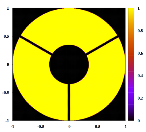
Figure 1: Pupil function of SNAP telescope. The outer radius is 1 meter and the inner radius is 0.35 meter. The width of the three secondary mirror supporting struts is 4 cm.

3.2 Optical Path Difference (OPD)

The OPD map of the perfectly aligned telescope and the derivatives with respect to misalignment parameters are calculated using ray tracing through the telescope’s optical system. The OPD is projected onto a Zernike basis, with results shown in Table 1.

$$OPD(\vec{\xi},\vec{\theta})=\sum_{n=1}\left[C_{n}(\vec{\theta})+\sum_{m}D_{m}C^{\prime}_{mn}(\vec{\theta})\right]Z_{n}(\vec{\xi})\,,$$ (16)

where $Z_{n}$ is the $n^{th}$ Zernike polynomial, $D_{m}$ is the the $m^{th}$ misalignment parameter, $C_{n}(\vec{\theta})$ is the OPD’s Zernike coefficients for pristine telescope and $C^{\prime}_{mn}(\vec{\theta})$ is the Zernike coefficients of ${{\partial OPD}\over{\partial D_{m}}}$.

In the SNAP telescope design (Lampton, 2002; Sholl et al, 2004), the secondary mirror position is expected to be the only optical dimension to vary significantly with time due to thermal drift. The secondary mirror has 5 degrees of freedom (DOF) which include shifts $D_{x}$ and $D_{y}$ in transverse directions, the defocus $D_{z}$, plus tilts around the $x$ axis ($T_{x}$) and $y$ axis ($T_{y}$).

In practice we find that $C^{\prime}_{mn}(\vec{\theta})$ is a very weak function of field for these parameters, and hence for the current simulation we take $C^{\prime}_{mn}$ to be constants. The pristine-telescope Zernike coefficients $C_{n}(\vec{\theta})$ retain field dependence, but the axisymmetry of telescope design reduces the freedom to the radial direction.

Table 1: Zernike coefficients of the OPD in nm for a perfectly aligned telescope with field location 10.4 mrad off axis $C_{n}$, and the derivatives $C^{\prime}_{mn}$ (see equation 16).

Zernike	2	3	4	5	6	7	8	9	10	11
$C_{n}$	7.75	0.00	10.87	0.00	8.43	0.00	-4.45	0.00	9.15	-0.88
$D_{x}$ ($\mu{\rm m}$)	-2.54	0.00	0.14	0.00	0.18	0.00	1.86	0.00	0.00	0.00
$D_{y}$ ($\mu{\rm m}$)	0.00	-2.55	0.00	-0.18	0.00	1.86	0.00	0.00	0.00	0.00
$D_{z}$ ($\mu{\rm m}$)	-0.08	0.00	-23.68	0.00	0.01	0.00	0.00	0.00	0.00	0.24
$T_{x}$ ($\mu{\rm rad}$)	0.00	1.27	0.00	0.63	0.00	-0.93	0.00	0.00	0.00	0.00
$T_{y}$ ($\mu{\rm rad}$)	-1.27	0.00	-0.48	0.00	0.64	0.00	0.93	0.00	0.00	0.00

3.3 Charge Diffusion

The optical PSF must be convolved with the charge-diffusion pattern of the CCD detector. Charge diffusion is modeled as a Gaussian with fixed charge diffusion length $\sigma_{d}=4\,\mu{\rm m}$. If the charge-diffusion length were free to vary, it would be degenerate with an isotropic telescope jitter (see below). The PSF after charge diffusion is

$$PSF(x,y)=\int dx^{\prime}dy^{\prime}PSF_{0}(x^{\prime},y^{\prime}){1\over{\sqrt{2\pi}\sigma_{d}}}{\rm exp}\left\{-{{(x-x^{\prime})^{2}+(y-y^{\prime})^{2}}\over{2\sigma_{d}^{2}}}\right\}\,,$$ (17)

where $PSF_{0}$ is the optical PSF. We execute the convolution with Fast Fourier Transforms (FFTs).

3.4 Jitter

Guiding errors and mirror vibrations, also known as jitter, alter the effective PSF of a finite-length exposure. Each exposure hence has a unique PSF map, even if the optics are otherwise stable. If the observatory is free to rotate on all three axes, as for a space-borne observatory or an alt-az terrestrial telescope, then the effect of jitter varies across the field of view, and is not a simple convolution of the image with a fixed kernel. Stellar images in the exposure can be used to infer the full field dependence of the jitter on the PSF. We demonstrate here that as few as two stars are sufficient to fully reconstruct the jittered PSFs, as long as the jitter amplitude is much less than the width of the PSF.

3.4.1 Effect of Jitter on the PSF

Assume that the modulation transfer function (MTF, the Fourier transform of the PSF) at ${\bf x}=(x,y)$ from the optic axis is known to be $T_{0}({\bf k})$ in the absence of telescope jitter. If the jitter has displaced the stellar image by some amount ${\bf\Delta x}=(\Delta x,\Delta y)$—which varies in time—then the transfer function becomes

$$T({\bf k},t)=T_{0}({\bf k})e^{-i{\bf k}\cdot{\bf\Delta x}(t)}\,.$$ (18)

The PSF for stellar images in the integrated exposure is the time-averaged value

$$T({\bf k})={1\over P}\int_{0}^{P}dtT({\bf k},t)=T_{0}({\bf k})\left<e^{-i{\bf k}\cdot{\bf\Delta x}(t)}\right>\,.$$ (19)

If ${\bf k}\cdot{\bf\Delta x}\ll 1$, then the exponential can be approximated by a Taylor expansion:

$$T({\bf k})=T_{0}({\bf k})\left[1-i{\bf k}\cdot\left<{\bf\Delta x}(t)\right>-{\bf k}^{T}\left<{\bf\Delta x\Delta x}^{T}\right>{\bf k}/2\right]\,.$$ (20)

The effect of the jitter on the PSF is then fully described by the mean displacement $\left<{\bf\Delta x}\right>$ and by the covariance matrix ${\bf C}_{\Delta x}=\left<{\bf\Delta x\Delta x}^{T}\right>$. Further detail of the jitter history is irrelevant. The linear term is simply a displacement of the entire PSF, and the quadratic term describes a convolution of the jitter-free PSF with a very narrow jitter kernel. With a telescope of diameter $D$, focal length $f$, and wavelength $\lambda$, physical optics forces MTF=0 for $k<2D/(\lambda f)$. Therefore the Taylor expansion is valid if

$${{2D\Delta x}\over{\lambda f}}\ll 1\,,$$ (21)

in other words the jitter must be much less than the size of the Airy disk.

3.4.2 Field Dependence of the Jitter MTF

If the observatory axis is displaced by angles $\mbox{\boldmath$\theta$}=(\theta_{x},\theta_{y},\theta_{z})$, i.e. pitch, yaw, and roll, then the displacement of the image of star $i$ at $(x_{i},y_{i})$ is

$$\Delta x_{i}=f\theta_{x}-y_{i}\theta_{z}$$ (22)

$$\Delta y_{i}=f\theta_{y}+x_{i}\theta_{z}\,.$$ (23)

If the roll is non-zero, then the image displacement is field-dependent. Now considering the observatory misalignment (jitter) to be a function of time,

$$\left<\Delta x_{i}\Delta x_{i}\right>=f^{2}\left<\theta_{x}\theta_{x}\right>-2fy_{i}\left<\theta_{x}\theta_{z}\right>+y_{i}^{2}\left<\theta_{z}\theta_{z}\right>$$ (24)

$$\left<\Delta x_{i}\Delta y_{i}\right>=f^{2}\left<\theta_{x}\theta_{y}\right>+fx_{i}\left<\theta_{x}\theta_{z}\right>-fy_{i}\left<\theta_{y}\theta_{z}\right>-x_{i}y_{i}\left<\theta_{z}\theta_{z}\right>$$ (25)

$$\left<\Delta y_{i}\Delta y_{i}\right>=f^{2}\left<\theta_{y}\theta_{y}\right>+2fx_{i}\left<\theta_{y}\theta_{z}\right>+x_{i}^{2}\left<\theta_{z}\theta_{z}\right>$$ (26)

In the small-jitter limit, therefore, we find that the effect of the jitter on the PSF at every point in the field of view is fully described by the six independent elements of the jitter covariance matrix ${\bf C}_{\theta}=\left<\mbox{\boldmath$\theta$}{\mbox{\boldmath$\theta$}}^{T}\right>$. We can write

$$T({\bf k},{\bf x})=T_{0}({\bf k},{\bf x})\left[1-{\bf k}\cdot{\bf C}_{\Delta x}({\bf C}_{\theta},{\bf x})\cdot{\bf k}/2\right]\,.$$ (27)

In practice, therefore, if we have an exposure for which the jitter-free PSF pattern is well determined, then we can completely determine the jittered PSF anywhere in the focal plane by knowing the elements of ${\bf C}_{\theta}$. The jitter covariance matrix could be determined from perfect knowledge of the PSF of any two stars in the exposure. If there are a larger number of stars in the exposure, then the six jitter covariances are highly over determined, hence they are easily derived for every exposure, even if there are other degrees of freedom in $T_{0}$ which must be determined from these stars.

If the jitter amplitude is not small, then there can be a much larger number of moments of the jitter history that are important, and a finite number of stellar images may not in general recover full knowledge of the effect of jitter on the PSF over the field. We will defer consideration of this limit for another paper.

4 Simulation Procedure

The simulation process is to: assume fiducial PSF parameters (misalignment and/or jitter); create simulated stellar images across the instrumented field of view; measure moments of these images; fit the PSF model to these moments; and finally, evaluate the quality of the fit.

4.1 Fiducial Model

We analyze a fiducial case in which the secondary mirror is translated 1 $\mu$m and rotated 1 $\mu$rad from its correct position. This would be considered a very large error for the optomechanical system. We have verified that the choice of fiducial model does not influence the RMS residuals to the fit.

When analyzing jitter, we assume an RMS motion of 36 mas in pitch and yaw with 700 mas RMS in roll (as expected from SNAP telescope design). The RMS cross-correlation between axes is taken to be small by comparison. Again, these do not strongly affect the results.

4.2 Simulated Stars

We use the star counts from the COSMOS HST survey as representative of high galactic latitude fields. The star counts in the COSMOS field (Robin et al, 2006) are well fit by (see Figure 2)

$${dn^{\star}\over dm}=18.5\times 10^{0.089m}\,{\rm deg^{-2}mag^{-1}}\,,$$ (28)

where $m$ is stellar magnitude in the F814W band.

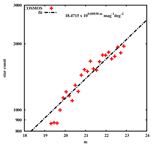
Figure 2: COSMOS survey star magnitude distribution (Robin et al, 2006).

If the star is too bright, it would saturate the SNAP CCDs. We hence conservatively assume that only stars with $19<m<23$ will be used for morphometry. The bright limit roughly corresponds to 50,000 photons for a 300 second exposure. The faint limit corresponds to $\approx 1200$ photons per star, which is comparable to the sky background in the exposure. Fainter stars will contribute little to the PSF knowledge.

The instrumented SNAP focal plane area is $\approx 0.7\,{\rm deg^{2}}$. This places approximately 2100 measurable stars on the focal plane, with a total photon count of $N_{\gamma}\approx 2.3\times 10^{7}$ per 300 sec exposure. This suggests that an ideal morphometry process would yield $e^{\rm RMS}$, $\sqrt{2}\sigma^{\rm RMS}_{\star}\sim 2\times 10^{-4}$, well below the required weak lensing specification as discussed in § 1.

We generate a sample of 2100 stars with random positions across the focal plane. The magnitude of the stars is randomly generated according to the magnitude distribution of equation 28. The PSF, including optical distortions and charge diffusion is computed, and is used to determine the mean number of photons detected in the CCD pixels. The number of detected photons per pixel is drawn from a Poisson distribution, and the quantum efficiency and gain of the SNAP pixels are used to compute pixel values. Random dark noise of 5 photo-electrons (as expected in the SNAP CCDs) is added to each pixel. The PSF moments defined in equations 1-6 and equation 9 are then computed from the pixel values.

4.3 Fitting Process

For each available star in an exposure, we calculate the second and third moments of a PSF image to which shot noise, sky noise, and read noise have been added. With the resulting PSF moments as data, we search for the best fit misalignment parameters by minimizing $\chi^{2}$

$$\chi^{2}=\sum_{i=1}^{N_{\star}}\sum_{jmom=1}^{Nmom}{{(M_{i}^{jmom}-\hat{M}_{i}^{jmom})^{2}}\over{\sigma_{moment}^{2}}}\,,$$ (29)

where $N_{\star}$ is the total number of stars, $Nmom$ is the number of independent PSF moments per star ($Nmom=3$ if only 2nd moments are used), $M$ is star moment (with noise), $\hat{M}$ is star moment calculated from the model (no noise), and $\sigma_{moment}$ is the rms of star moments. In general, $\sigma_{moment}$ depends on star magnitude, filter band and the position of the star on the focal plane. We assume a fixed filter band and neglect the ($<10\%$) dependence on position. We produce a lookup table of $\sigma_{moment}$ vs source magnitude by Monte Carlo methods before doing the fit.

The PSF moments depend nonlinearly on misalignment parameters. As an example, Figure 3 shows the dependence of $P_{xx}$ on the defocus parameter $D_{z}$. The model-fitting procedure is hence nonlinear, so slower than a linear $\chi^{2}$ fit.

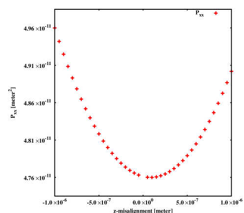
Figure 3: Dependence of PSF moment $P_{xx}$ on $z$-misalignment (in meters). The star is located on the diagonal (i.e. $x=y$).

5 Results

In this section, we show results of simulating and fitting for secondary mirror misalignment only, and simulating and fitting with the jitter parameters jointly. We also show that the inclusion of third moments of the PSFs improves the fit.

5.1 Fit for Secondary Misalignments Only

5.1.1 Using Second Moments of PSFs

We first simulate a single exposure of SNAP, using only the PSF second moments to constrain the secondary-mirror misalignment. The fiducial misalignment parameters, their fitted values, and the $1-\sigma$ uncertainties are listed in Table 2. $D_{z}$ is precise to $<10$ nm which is well below the achievable mechanical stability. Hence the morphometric information can greatly improve knowledge of defocus. The other parameters are as much as 20 times less precise: accuracies of $\approx 0.2\,\mu$m in $D_{x}$ and $D_{y}$ seem quite disappointing, for example.

Table 2: Misalignment fitting results

misalignment	fiducial value	fitted value	$1-\sigma$ error	fit incl. 3rd moments	$1-\sigma$ error
$D_{x}$ ($\mu{\rm m}$)	1	0.8542	0.1839	1.0052	0.1494
$D_{y}$ ($\mu{\rm m}$)	-1	-1.3869	0.2020	-1.0719	0.1602
$D_{z}$ ($\mu{\rm m}$)	1	0.9870	0.0086	1.0005	0.0083
$T_{x}$ ($\mu{\rm rad}$)	1	0.4500	0.3280	0.8104	0.3125
$T_{y}$ ($\mu{\rm rad}$)	1	1.2370	0.3063	0.8549	0.2937

To better understand this wide range of precisions, we examine the eigenvectors and eigenvalues of the parameter covariance matrix, shown in Table 3. The best-constrained eigenvector is along the $D_{z}$ direction, i.e. defocus. Two eigenvectors are $\approx 80$ times more poorly constrained, but this is not hard to understand. If the secondary mirror were spherical with radius $R$, it would have only three degrees of freedom, as misalignments with $D_{x}=-RT_{y}$ and $D_{y}=-RT_{x}$ leave the sphere invariant. A non-spherical secondary mirror breaks these degeneracies and results in finite (but poor) constraints on these eigenvectors.

Table 3: Eigen values and eigen vectors of the misalignment covariance matrix

	eigen 1	eigen 2	eigen 3	eigen 4	eigen 5
$D_{x}$ ($\mu{\rm m}$)	0.0661	0.4852	0.7423	0.4573	0.0037
$D_{y}$ ($\mu{\rm m}$)	-0.5022	0.0535	0.4597	-0.7304	-0.0107
$D_{z}$ ($\mu{\rm m}$)	0.0033	0.0189	-0.0058	-0.0191	0.9996
$T_{x}$ ($\mu{\rm rad}$)	-0.8502	0.1516	-0.2812	0.4185	0.0063
$T_{y}$ ($\mu{\rm rad}$)	-0.1438	-0.8593	0.3981	0.2862	0.0245
eigen values ($\lambda_{i}\times 10^{6}$)	0.3781	0.3479	0.0797	0.0758	0.0052
Residual ($\times 10^{6}$)	0.6180	-0.3789	-0.0370	0.0538	-0.0071

The “Residual” row in the table gives the projection of the fitting error onto the eigenvectors. It shows that the fitted parameters deviate from the fiducial mostly in the directions that have weak constraints. All the deviations are at or below $1.6\,\sigma$ level which is a sign that the fitter is working properly.

The quantity that matters to weak lensing is the precision of the PSF knowledge. The apparent poor fit to some of the misalignments reflects the insensitivity of the PSF moments to certain combinations. This insensitivity also means, however, that poor knowledge of these eigenvectors has little adverse effect on our PSF model. We compare the noiseless PSF ellipticities and size generated using the fitted misalignment parameters with these generated using fiducial misalignment parameters. Figure 4 (left panel) shows the distributions of the residual PSF moments for a realization of a single exposure. We see that the PSF errors are well below the $10^{-3}$ target for all three quantities. The spread in PSF errors reflects the variation across the focal plane.

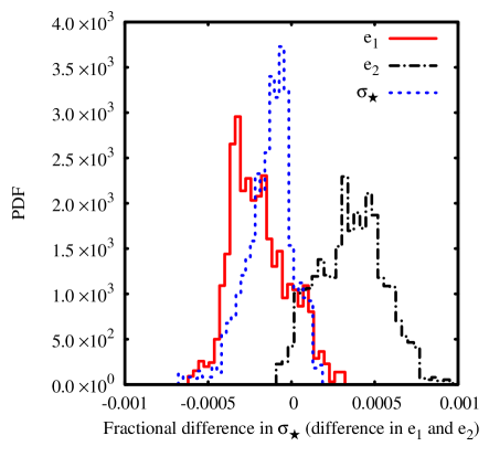
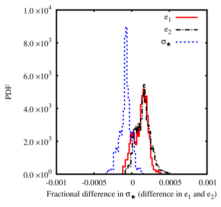
Figure 4: Distributions of the residual PSF moments as defined in the text. Left panel: the fit is done using 2nd moments of the PSFs. Right panel: both 2nd and 3rd moments of the PSFs are used.

5.1.2 Including Higher Moments of PSFs

There is information in the higher moments of the PSF. This could further constrain the telescope misalignments. As shown in Table 2, the fitted misalignments are noticeably closer to the true values and the error bars are reduced when the observed PSF second and third moments are used in the misalignment fit. Figure 4 shows the reduction in PSF ellipticity and size residuals. With the inclusion of third moments in the fit, the reduction of the residual moments as shown in Figure 4 are much more impressive than that of the one sigma errors shown in Table 2. This is the manifestation that the contributions to the one sigma errors are dominated by the two near degenerate eigens which have little or no effect on the residual PSF moments. In the following, we include third moments in the fit unless stated otherwise.

5.2 Fitting Misalignment and Jitter Parameters Jointly

Table 4 shows the results of fitting secondary misalignment and jitter parameters jointly. Adding the 6 jitter degrees of freedom to the model roughly doubles the uncertainties on the 5 misalignment degrees of freedom. The parameter $D_{z}$ is still very precise (at $20\,{\rm nm}$ level). The jitter parameters are determined without significant degeneracies among each other nor with the misalignments; this is because these parameters influence the PSF moments with rather distinct dependences on field angle.

Table 4: Fitting for misalignment and jitter parameters

parameters	fit incl. 3rd moments	fiducial values	$1-\sigma$ error
$D_{x}$ ($\mu{\rm m}$)	0.5367	1	0.3596
$D_{y}$ ($\mu{\rm m}$)	-0.1932	-1	0.3763
$D_{z}$ ($\mu{\rm m}$)	0.9725	1	0.0203
$T_{x}$ ($\mu{\rm rad}$)	2.6843	1	0.7503
$T_{y}$ ($\mu{\rm rad}$)	1.9457	1	0.7207
$\left<\theta_{x}\theta_{x}\right>$ ($\mu{\rm rad}^{2}$)	0.0302	0.0300	0.0002
$\left<\theta_{x}\theta_{y}\right>$ ($\mu{\rm rad}^{2}$)	0.0013	0.0010	0.0001
$\left<\theta_{x}\theta_{z}\right>$ ($\mu{\rm rad}^{2}$)	0.0049	0.0010	0.0045
$\left<\theta_{y}\theta_{y}\right>$ ($\mu{\rm rad}^{2}$)	0.0298	0.0300	0.0002
$\left<\theta_{y}\theta_{z}\right>$ ($\mu{\rm rad}^{2}$)	-0.0011	0.0010	0.0046
$\left<\theta_{z}\theta_{z}\right>$ ($\mu{\rm rad}^{2}$)	19.5098	20.0000	0.9244

The residual PSF ellipticities and sizes for one realization of joint misalignment/jitter fitting are shown in Figure 5.

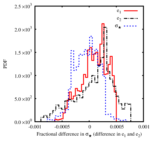
Figure 5: Distributions of the residual PSF moments for fit including 5 secondary mirror misalignment and 6 jitter parameters. Both 2nd and 3rd moments of the PSF are utilized.

As mentioned before, the spreads of the residual PSF $e_{1},e_{2}$, and $\sigma_{\star}$ distributions in this single realization are due to field dependence. Different realizations of the data (star locations and random noise change) produce different mean and spread of the residual moments distribution. Figure 6 left panel shows the distributions of $e^{\rm RMS}$ and $\sigma_{\star}^{\rm RMS}$ from 50 realizations. We produce a single measure of the efficacy of the morphometry procedure by averaging the RMS PSF residuals over all focal-plane positions in many realizations, as per equations 10-12. The mean values (in quadrature) of the distributions in Figure 6 left panel are exactly those. They are labeled by the arrows in the plot and listed in Table 5 as well. Calculated using equation 13, the $\alpha$ values are also tabulated in Table 5. Taking the average value, we find $\alpha\approx 1.8$. So we have

$$e_{1}^{\rm RMS}\approx e_{2}^{\rm RMS}\approx\sqrt{2}\sigma_{\star}^{\rm RMS}=1.8N_{\gamma}^{-1/2}\,.$$ (30)

The ensemble average residuals are consistent with zero, i.e. the PSF models are unbiased, to the $2.5\times 10^{-5}$ accuracy of our 50 realizations.

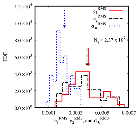
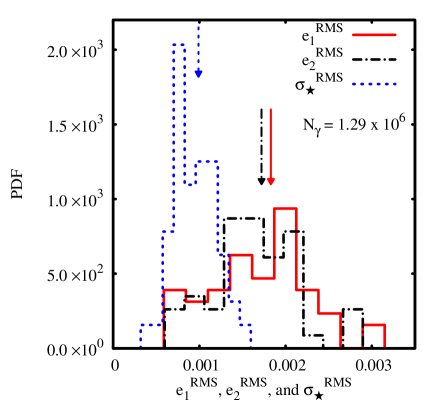
Figure 6: Distributions of $e_{1}^{\rm RMS}$, $e_{2}^{\rm RMS}$, and $\sigma_{\star}^{\rm RMS}$ from 50 realizations. Left: 2100 stars are used for each realization. Right: 100 stars are used for each realization. The arrows point at the quadrature means of the distributions which are listed in Table 5. Note that the horizontal scales are different in the two panels.

Table 5: Average $e^{\rm RMS}$ and $\sigma_{\star}^{\rm RMS}$ from 50 realizations and $\alpha$ values

	2100 stars per realization	$N_{\gamma}=2.37\times 10^{7}$	100 stars per realization	$N_{\gamma}=1.29\times 10^{6}$
	average	$\alpha$	average	$\alpha$
$e_{1}^{\rm RMS}$	$4.0\times 10^{-4}$	1.95	$1.8\times 10^{-3}$	2.04
$e_{2}^{\rm RMS}$	$3.9\times 10^{-4}$	1.90	$1.7\times 10^{-3}$	1.93
$\sigma_{\star}^{\rm RMS}$	$2.2\times 10^{-4}$	1.52	$1.0\times 10^{-3}$	1.14

To test our hypothesis that the PSF errors will scale as $N_{\gamma}^{-1/2}$, we repeat the simulation using 100 stars instead of the fiducial 2100 stars. The distributions of $e^{\rm RMS}$ and $\sigma_{\star}^{\rm RMS}$ are shown in the right panel of Figure 6. Again, the quadrature means of these distributions are labeled by the arrows in the plot and listed in Table 5. We find $\alpha\approx 1.7$. So the RMS residuals do indeed scale as expected.

From Figure 5 it is clear that part of the residual errors in the PSF ellipticities are from a shift in the mean across the field of view, while the rest is from errors that vary across the field of view. The two different types of PSF modeling errors will propagate into different angular scales in the WL power spectrum. For the SNAP simulation, we find that roughly half of the $e$ modeling variance is in the mean across the field of view.

Since essentially all the residual variance arises from shot noise in the stars, it will be uncorrelated from exposure to exposure.

6 Conclusion and Discussion

Our simulation of “morphometry” for the SNAP telescope demonstrates that the $\approx 2000$ well-measured stars in a typical exposure contain sufficient information to reduce the errors in the modeled PSF ellipticity and size to $4.0\times 10^{-4}$ and $2.2\times 10^{-4}$ respectively, giving significant margin to meet the $\approx 10^{-3}$ level needed to reduce weak-lensing systematic errors below statistical errors of future surveys. For the SNAP telescope design and focal plane, we find $e^{\rm RMS}\approx 1.8/\sqrt{N_{\gamma}}$ and $\sigma_{\star}^{\rm RMS}\approx 1.1/\sqrt{N_{\gamma}}$.

PSF estimation error in morphometry will be only part of the shape-measurement error budget, so this margin is important. Other potential source of errors in PSF estimation include charge transfer inefficiency (CTI), data compression artifacts, and chromatic PSF dependence that causes galaxies’ PSFs to differ from stellar PSFs. Shape measurement errors can also arise in the deconvolution process even if the PSF is known precisely (Heymans et al, 2006; Massey et al, 2007). To have a successful weak lensing mission, the sum of these errors must meet the weak lensing requirement.

We have also assumed that the only time-variable aspects of the PSF are the secondary mirror alignment, and small pointing jitter. The SNAP spacecraft is engineered to take advantage of the extremely stable space environment so that these are the only relevant degrees of freedom. A ground based observatory would suffer in addition the effects of wind, gravity loading, and seeing, which are complicated to model, potentially involving a large number of degrees of freedom. We have seen in the SNAP case that adding 6 jitter degrees of freedom to the PSF model makes the PSF model errors twice as large as when we fit for only 5 misalignment parameters, so it seems likely that the PSF modeling performance will be degraded by larger number of parameters in the system.

References

- Amara & Refregier (2007) Amara, A., & Refregier, A., 2007, astro-ph/0710.5171
- Bartelmann & Schneider (2001) Bartelmann, M., & Schneider, P., 2001, Phys. Rept. 340, 291 (astro-ph/9912508)
- Bernardeau (1998) Bernardeau, F., 1998, Astron. & Astrophys. 338, 375-382 (astro-ph/9712115)
- Bernstein (2008) Bernstein, G., 2008, astro-ph/0808.3400
- Bridle & King (2007) Bridle, S., & King, L., 2007, New Journal of Physics, Vol. 9, Issue 12, 444 (astro-ph/0705.0166)
- Cimatti et al (2008) Cimatti, A., Robberto, M., & Baugh, C.M. et al, 2008, astro-ph/0804.4433
- Cooray & Hu (2002) Cooray, A., & Hu, W., 2002, ApJ 574, 19 (astro-ph/0202411)
- Dodelson et al (2006) Dodelson, S., Shapiro, C., & White, M., 2006, Phys. Rev. D73, 023009 (astro-ph/0508296)
- Hamana (2001) Hamana, T., 2001, MNRAS 326, 326 (astro-ph/0104244)
- Heymans & Heavens (2003) Heymans, C., & Heavens, A., et al, 2003, MNRAS 339, 711 (astro-ph/0208220)
- Heymans et al (2006) Heymans, C., Waerbeke, L., & Bacon, D. et al, 2006, MNRAS 368, 1323-1339 (astro-ph/0506112)
- Heymans et al (2006) Heymans, C., White, M., & Heavens, A. et al, 2006, MNRAS 371, 750-760 (astro-ph/0604001)
- Hirata et al (2007) Hirata, C., Mandelbaum, R., & Ishak M. et al, 2007, MNRAS 381, 1197-1218 (astro-ph/0701671)
- Hirata & Seljak (2004) Hirata, C., & Seljak, U., 2004, Phys. Rev. D70, 063526 (astro-ph/0406275)
- Huterer & Takada (2005) Huterer, D., & Takada, M., 2005, Astropart. Phys. 23, 369-376 (astro-ph/0412142)
- Huterer et al (2006) Huterer, D., Takada, M., Bernstein, G., & Jain, B., 2006, MNRAS 366, 101-114 (astro-ph/0506030)
- Jain et al (2006) Jain, B., Jarvis, M., & Bernstein, G., 2006, JCAP 0602, 001 (astro-ph/0412234)
- Jarvis & Jain (2004) Jarvis, M., & Jain, B., 2004, astro-ph/0412234
- Joachimi & Schneider (2008) Joachimi, B., & Schneider, P., 2008, astro-ph/0804.2292
- Kaiser (1998) Kaiser, N., 1998, ApJ, 498, 26 (astro-ph/9610120)
- King (2006) King, L., 2005, astro-ph/0506441
- King & Schneider (2002) King, L., & Schneider, P., 2002, Astron. Astrophys. 396, 411-418 (astro-ph/0208256)
- King & Schneider (2003) King, L., & Schneider, P., 2003, Astron. Astrophys. 398:23-30 (astro-ph/0209474)
- Lampton (2002) Lampton, M., 2002, astro-ph/0209549
- Lee & Pen (2008) Lee, J., & Pen, U., 2008, ApJ 681, 798-806 (astro-ph/0707.1690)
- Ma & Bernstein (2008) Ma, Z., & Bernstein, G., 2008, ApJ 682, 39-48 (astro-ph/0712.1562)
- Ma et al (2006) Ma, Z., Hu, W., & Huterer, D., 2006, ApJ 636, 21-29 (astro-ph/0506614)
- Mandelbaum et al (2006) Mandelbaum, R., Hirata, C., & Ishak, M. et al, 2006, MNRAS 367, 611-626 (astro-ph/0509026)
- Massey et al (2007) Massey, R., Heymans, C., & Berge, J. et al, 2007, MNRAS 376, 13-38 (astro-ph/0608643)
- Noll (1976) Noll, R. J., 1976, J. Opt. Soc. Am., Vol. 66, No. 3