A Local Construction of the Smith Normal Form of a Matrix Polynomial

Abstract

We present an algorithm for computing a Smith form with multipliers of a regular matrix polynomial over a field. This algorithm differs from previous ones in that it computes a local Smith form for each irreducible factor in the determinant separately and then combines them into a global Smith form, whereas other algorithms apply a sequence of unimodular row and column operations to the original matrix. The performance of the algorithm in exact arithmetic is reported for several test cases.

1 Introduction

Canonical forms are a useful tool for classifying matrices, identifying their key properties, and reducing complicated systems of equations to the de-coupled, scalar case. When working with matrix polynomials over a field $K$, one fundamental canonical form, the Smith form, is defined. It is a diagonalization

$$A(\lambda)=E(\lambda)D(\lambda)F(\lambda)$$ (1)

of the given matrix $A(\lambda)$ by unimodular matrices $E(\lambda)$ and $F(\lambda)$ such that the diagonal entries $d_{i}(\lambda)$ of $D(\lambda)$ are monic polynomials and $d_{i}(\lambda)$ is divisible by $d_{i-1}(\lambda)$ for $i\geq 2$.

This factorization has various applications. The most common one Goh1982 ; kailath80 ; neven93 involves solving the system of differential equations

$$A^{(q)}\frac{d^{q}x}{dt^{q}}+\dots+A^{(1)}\frac{dx}{dt}+A^{(0)}x=f(t),$$ (2)

where $A^{(0)}$, …, $A^{(q)}$ are $n\times n$ matrices over $\mathbb{C}$. For brevity, we denote this system by $A(d/dt)x=f$, where $A(\lambda)=A^{(0)}+A^{(1)}\lambda+\dots+A^{(q)}\lambda^{q}$. Assume for simplicity that $A(\lambda)$ is regular, i.e. $\det[A(\lambda)]$ is not identically zero, and that (1) is a Smith form of $A(\lambda)$. The system (2) is then equivalent to

$$\left(\begin{array}[]{ccc}d_{1}(\frac{d}{dt})&&\\ &\ddots&\\ &&d_{n}(\frac{d}{dt})\\ \end{array}\right)\left(\begin{array}[]{c}y_{1}\\ \vdots\\ y_{n}\\ \end{array}\right)=\left(\begin{array}[]{c}g_{1}\\ \vdots\\ g_{n}\\ \end{array}\right),$$

where $y=F(d/dt)x(t)$ and $g=E^{-1}(d/dt)f(t)$. Note that $E^{-1}(\lambda)$ is a matrix polynomial over $\mathbb{C}$ due to the unimodularity of $E(\lambda)$. This system splits into $n$ independent scalar ordinary differential equations

$$d_{i}\Big{(}\frac{d}{dt}\Big{)}y_{i}(t)=g_{i}(t),\qquad 1\leq i\leq n,$$

and the solution of (2) is then given by $x=F^{-1}(d/dt)y$, where $F^{-1}(\lambda)$ is also a matrix polynomial over $\mathbb{C}$.

Another important application of the Smith form concerns the study of the algebraic structural properties of systems in linear control theory kailath80 ; rosenbrock70 ; vanDooren83 . For example, the zeros and poles of a multivariable transfer function $H(s)$ are revealed by the Smith-McMillan form of $H(s)$, which is a close variant of the Smith form, but for rational (as opposed to polynomial) matrices. In many applications, one only needs to compute a minimal basis for the kernel of a matrix polynomial. Specialized algorithms neven93 ; zuniga09 have been developed for this sub-problem of the Smith form calculation.

Smith forms of linear matrix polynomials (i.e. matrix pencils) are related to the concept of similarity of matrices. A fundamental theorem in matrix theory Gant1960 ; Goh1982 states that two square matrices $A$ and $B$ over a field $K$ are similar if and only if their characteristic matrix polynomials $\lambda I-A$ and $\lambda I-B$ have the same Smith form $D(\lambda)$. Other applications of this canonical form include finding the Frobenius form Villard94 ; Villard1997 of a matrix $A$ over a field by computing the invariant factors of the matrix pencil $\lambda I-A$.

Many algorithms have been developed for the computation of canonical forms of matrix polynomials in floating point arithmetic. One common approach involves finding an equivalent linear matrix pencil with the same finite zeros as the original matrix polynomial and a closely related Smith form vanDooren83 . The Kronecker form vanDooren79 ; vanDooren83 ; demmel of the matrix pencil is then computed to determine the eigenstructure of the original polynomial matrix. Another approach centers around computing the local spectral structure of a matrix polynomial at a single complex root, $\lambda_{0}$, of the characteristic determinant vanSchagen ; Wilken2007 . These methods usually boil down to computing kernels of nested Toeplitz matrices Wilken2007 ; zuniga09 . One advantage of this local approach over the global matrix pencil approach is that only a few terms in an expansion of the matrix polynomial in powers of $\lambda-\lambda_{0}$ are needed to compute the spectral behavior. This can lead to a significant computational savings, and also allows for generalization from matrix polynomials to analytic matrix functions vanSchagen ; Wilken2007 . Such local canonical forms can be used to efficiently compute successive terms in the Laurent expansion of the inverse of an analytic matrix howlett ; Wilken2007 . Backward stability analysis of the effect of roundoff error may be found in vanDooren83 ; Wilken2007 ; zuniga09 . A geometric approach to the perturbation theory of matrix pencils is discussed in edelman1 .

The symbolic computation of Smith forms of matrices over $\mathbb{Q}[\lambda]$ is also a widely studied topic. Kannan Kann1985 gave a method for computing the Smith form with repeated triangularizations of the matrix polynomial over $\mathbb{Q}$. Kaltofen, Krishnamoorthy and Saunders Kal1987 gave the first polynomial time algorithm for the Smith form (without multipliers) using the Chinese remainder theorem. A new class of probabilistic algorithms (the Monte Carlo algorithms) were proposed by Kaltofen, Krishnamoorthy and Saunders Kal1987 ; Kal1990 . They showed that by multiplying the given matrix polynomial by a randomly generated constant matrix on the right, the Smith form with multipliers is obtained with high probability by two steps of computation of the Hermite form. A Las Vegas algorithm given by Storjohann and Labahn Stor1994 ; Stor1997 significantly improved the complexity by rapidly checking the correctness of the result of the KKS algorithm. Villard Villard93 ; Villard95 established the first deterministic polynomial-time method to obtain the Smith form with multipliers by explicitly computing a good-conditioning matrix that replaces the random constant matrix in the Las Vegas algorithm. Villard also applied the method of Marlin, Labhalla and Lombardi lab1996 to obtain useful complexity bounds for the algorithm.

We propose a new deterministic algorithm for the symbolic computation of Smith forms of matrix polynomials over a field in Section 3. Our approach differs from previous methods in that we begin by constructing local diagonal forms that we later combine to obtain a (global) post-multiplier. Although we do not discuss complexity bounds, we compare the performance of our algorithm to Villard’s method with good conditioning in Section 4, and discuss the reasons for the increase in speed. The new algorithm is also easy to parallelize. In Appendix A, we present an algebraic framework that connects this work to Wilken2007 , and give a variant of the algorithm in which all operations are done in the field $K$ rather than manipulating polynomials directly.

As mentioned above, local canonical forms have been used successfully to study the structure of a matrix polynomial near a single root $\lambda_{0}\in\mathbb{C}$ of the characteristic determinant. An important point that has been neglected in the literature is that these roots $\lambda_{0}$ may not be expressible in radicals, or may involve such complicated expressions that current algorithms can only be carried out in floating point arithmetic. A major goal of this paper is to develop a machinery for computing local forms for all the complex roots of a $\mathbb{Q}$-irreducible factor $p(\lambda)$ of the characteristic determinant simultaneously, without having to resort to floating point arithmetic at each root separately. This is done by working over the fields $\mathbb{Q}$ or $\mathbb{Q}+i\mathbb{Q}$ rather than $\mathbb{R}$ or $\mathbb{C}$ when computing local forms.

2 Preliminaries

In this section, we describe the theory of Smith forms of matrix polynomials over a field $K$, which follows the definition in Goh1982 over $\mathbb{C}$. In practice, $K$ will be $\mathbb{Q}$, $\mathbb{Q}+i\mathbb{Q}$, $\mathbb{R}$, or $\mathbb{C}$, but it is convenient to deal with all these cases simultaneously. We also give a brief review of the theory of Jordan chains as well as Bézout’s identity, which play an important role in our algorithm for computing Smith forms of matrix polynomials.

2.1 Smith Forms

Suppose $A(\lambda)=\sum_{k=0}^{q}A^{(k)}\lambda^{k}$ is an $n\times n$ matrix polynomial, where $A^{(k)}$ are $n\times n$ matrices whose entries are in a field $K$. Assuming that $A(\lambda)$ is regular, i.e. the determinant of $A(\lambda)$ is not identically zero, the following theorem is proved in Goh1982 (for $K=\mathbb{C}$).

Theorem 1.

There exist matrix polynomials $E(\lambda)$ and $F(\lambda)$ over $K$ of size $n\times n$, with constant nonzero determinants, such that

$$A(\lambda)=E(\lambda)D(\lambda)F(\lambda),\qquad D(\lambda)=\operatorname{diag}[d_{1}(\lambda),\dots,d_{n}(\lambda)],$$ (3)

where $D(\lambda)$ is a diagonal matrix with monic scalar polynomials $d_{i}(\lambda)$ over $K$ such that $d_{i}(\lambda)$ is divisible by $d_{i-1}(\lambda)$.

Since $E(\lambda)$ and $F(\lambda)$ have constant nonzero determinants, (3) is equivalent to

$$U(\lambda)A(\lambda)V(\lambda)=D(\lambda),$$ (4)

where $U(\lambda):=E(\lambda)^{-1}$ and $V(\lambda):=F(\lambda)^{-1}$ are also matrix polynomials over $K$.

Definition 2.

The representation in (3) or (4), or often $D(\lambda)$ alone, is called a Smith form of $A(\lambda)$. The matrices $U(\lambda)$, $V(\lambda)$ are known as multipliers. Square matrix polynomials with constant nonzero determinants like $E(\lambda)$ and $F(\lambda)$ are called unimodular.

The diagonal matrix $D(\lambda)$ in the Smith form is unique, while the representation (3) is not. Suppose that

$$\Delta(\lambda):=\det[A(\lambda)]$$ (5)

can be decomposed into prime elements $p_{1}(\lambda),\dots,p_{l}(\lambda)$ in the principal ideal domain $K[\lambda]$, that is, $\Delta(\lambda)=c\prod_{j=1}^{l}p_{j}(\lambda)^{\kappa_{j}}$ where $c\neq 0$ is in the field $K$, $p_{j}(\lambda)$ is monic and irreducible, and $\kappa_{j}$ are positive integers for $j=1,\dots,l$. Then the $d_{i}(\lambda)$ are given by

$$d_{i}(\lambda)=\prod_{j=1}^{l}p_{j}(\lambda)^{\kappa_{ji}},\qquad(1\leq i\leq n)$$

for some integers $0\leq\kappa_{j1}\leq\dots\leq\kappa_{jn}$ satisfying $\sum_{i=1}^{n}\kappa_{ji}=\kappa_{j}$ for $j=1,\dots,l$.

We now define a local Smith form for $A(\lambda)$ at $p(\lambda)$. Let $p(\lambda)=p_{j}(\lambda)$ be one of the irreducible factors of $\Delta(\lambda)$ and define $\alpha_{i}=\kappa_{ji}$, $\mu=\kappa_{j}$. Generalizing the case that $p(\lambda)=\lambda-\lambda_{j}$, we call $\mu$ the algebraic multiplicity of $p(\lambda)$.

Theorem 3.

Suppose $A(\lambda)$ is an $n\times n$ matrix over $K[\lambda]$ and $p(\lambda)$ is an irreducible factor of $\Delta(\lambda)$. There exist $n\times n$ matrix polynomials $E(\lambda)$ and $F(\lambda)$ such that

$$A(\lambda)=E(\lambda)D(\lambda)F(\lambda),\qquad D(\lambda)=\operatorname{diag}[p(\lambda)^{\alpha_{1}},\dots,p(\lambda)^{\alpha_{n}}],$$ (6)

where $0\leq\alpha_{1}\leq\dots\leq\alpha_{n}$ are non-negative integers and $p(\lambda)$ does not divide $\det[E(\lambda)]$ or $\det[F(\lambda)]$.

$E(\lambda)$ and $F(\lambda)$ are not uniquely determined in a local Smith form. In particular, we can impose the additional requirement that $F(\lambda)$ be unimodular by absorbing the missing parts of $D(\lambda)$ in Theorem 1 into $E(\lambda)$. Then the local Smith form of $A(\lambda)$ at $p(\lambda)$ is given by

$$A(\lambda)V(\lambda)=E(\lambda)D(\lambda),$$ (7)

where $V(\lambda):=F(\lambda)^{-1}$ is a matrix polynomial.

2.2 Multiplication and division in $R/pR$

We define $R=K[\lambda]$ and $M=R^{n}$. Note that $R$ is a principal ideal domain and $M$ is a free $R$-module of rank $n$. Suppose $p$ is a prime element in $R$. Since $p$ is irreducible, $R/pR$ is a field and $M/pM$ is a vector space over this field.

Multiplication and division in $R/pR$ are easily carried out using the companion matrix of $p$. If we set $s:=\deg p$ and define $\gamma:K^{s}\rightarrow R/pR$ by

$$\gamma(x)(\lambda)=x^{(0)}+\cdots+\lambda^{s-1}x^{(s-1)}+pR,\qquad x=\big{(}x^{(0)};\dots;x^{(s-1)}\big{)}\in K^{s},$$ (8)

we can pull back the field structure of $R/pR$ to $K^{s}$ to obtain

$$xy=\gamma(x)(S)y =[x^{(0)}I+x^{(1)}S+\cdots+x^{(s-1)}S^{s-1}]y$$ (9)

$$=[y,Sy,\dots,S^{s-1}y]x=[x,Sx,\dots,S^{s-1}x]y$$

and $x/y=[y,Sy,\dots,S^{s-1}y]^{-1}x$, where

$$S=\left(\begin{array}[]{cccc}0&\ldots&0&-a_{0}\\[-1.0pt] 1&\ddots&\vdots&\vdots\\[-5.0pt] &\ddots&0&-a_{s-2}\\ 0&&1&-a_{s-1}\end{array}\right)$$ (10)

is the companion matrix of $p(\lambda)=a_{0}+a_{1}\lambda+\cdots+a_{s-1}\lambda^{s-1}+\lambda^{s}$. Note that $S$ represents multiplication by $\lambda$ in $R/pR$. The matrix $[y,Sy,\dots,S^{s-1}y]$ is invertible when $y\neq 0$ since a non-trivial vector $x$ in its kernel would lead to non-zero polynomials $\gamma(x),\gamma(y)\in R/pR$ whose product is zero (mod $p$), which is impossible as $p$ is irreducible.

2.3 Jordan Chains

Finding a local Smith form of a matrix polynomial over $\mathbb{C}$ at $p(\lambda)=\lambda-\lambda_{0}$ is equivalent to finding a canonical system of Jordan chains vanSchagen ; Wilken2007 for $A(\lambda)$ at $\lambda_{0}$. We now generalize the notion of Jordan chain to the case of an irreducible polynomial over a field $K$.

Definition 4.

Suppose $A(\lambda)$ is an $n\times n$ matrix polynomial over a field $K$, $p(\lambda)$ is irreducible in $K[\lambda]$, and $\alpha\geq 1$ is an integer. A vector polynomial $x(\lambda)\in M=K[\lambda]^{n}$ is called a root function of order $\alpha$ for $A(\lambda)$ at $p(\lambda)$ if

$$A(\lambda)x(\lambda)=O(p(\lambda)^{\alpha})$$ (11)

and $p(\lambda)\nmid x(\lambda)$. The meaning of (11) is that each component of $A(\lambda)x(\lambda)$ is divisible by $p(\lambda)^{\alpha}$. If the root function $x(\lambda)$ has the form

$$x(\lambda)=x^{(0)}(\lambda)+p(\lambda)x^{(1)}(\lambda)+\cdots+p(\lambda)^{\alpha-1}x^{(\alpha-1)}(\lambda)$$ (12)

with $\deg x^{(k)}(\lambda)<s:=\deg p(\lambda)$, the coefficients $x^{(k)}(\lambda)$ are said to form a Jordan chain of length $\alpha$ for $A(\lambda)$ at $p(\lambda)$. A root function can always be converted to the form (12) by truncating or zero-padding its expansion in powers of $p(\lambda)$. If $K$ can be embedded in $\mathbb{C}$, (11) implies that over $\mathbb{C}$, $x(\lambda)$ is a root function of $A(\lambda)$ of order $\alpha$ at each root $\lambda_{j}$ of $p(\lambda)$ simultaneously.

Definition 5.

Several vector polynomials $\{x_{j}(\lambda)\}_{j=1}^{\nu}$ form a system of root functions at $p(\lambda)$ if

$$\begin{array}[]{l}1.\,\,A(\lambda)x_{j}(\lambda)=O(p(\lambda)^{\alpha_{j}}),\qquad(\alpha_{j}\geq 1,\quad 1\leq j\leq\nu)\\[3.0pt] \parbox{346.89731pt}{$2.$ The set $\{\dot{x}_{j}(\lambda)\}_{j=1}^{\nu}$ is linearly independent in $M/pM$ over $R/pR$, \\ \hskip 93.95122pt where $R=K[\lambda]$, $M=R^{n}$, $\dot{x}_{j}=x_{j}+pM$.}\end{array}$$ (13)

It is called canonical if (1) $\nu=\dim\ker\dot{A}$, where $\dot{A}$ is the linear operator on $M/pM$ induced by $A(\lambda)$; (2) $x_{1}(\lambda)$ is a root function of maximal order $\alpha_{1}$; and (3) for $i>1$, $x_{i}(\lambda)$ has maximal order $\alpha_{i}$ among all root functions $x(\lambda)\in M$ such that $\dot{x}$ is linearly independent of $\dot{x}_{1},\dots,\dot{x}_{i-1}$ in $M/pM$. The integers $\alpha_{1}\geq\dots\geq\alpha_{\nu}$ are uniquely determined by $A(\lambda)$. We call $\nu$ the geometric multiplicity of $p(\lambda)$.

Definition 6.

An extended system of root functions $x_{1}(\lambda)$,…,$x_{n}(\lambda)$ is a collection of vector polynomials satisfying (13) with $\nu$ replaced by $n$ and $\alpha_{j}$ allowed to be zero. The extended system is said to be canonical if, as before, the orders $\alpha_{j}$ are chosen to be maximal among root functions not in the span of previous root functions in $M/pM$. The resulting sequence of numbers $\alpha_{1}\geq\cdots\geq\alpha_{\nu}\geq\alpha_{\nu+1}=\cdots=\alpha_{n}=0$ is uniquely determined by $A(\lambda)$.

Given such a system (not necessarily canonical), we define the matrices

$$V(\lambda) =[x_{1}(\lambda),\dots,x_{n}(\lambda)],$$ (14)

$$D(\lambda) =\operatorname{diag}[p(\lambda)^{\alpha_{1}},\dots,p(\lambda)^{\alpha_{n}}],$$ (15)

$$E(\lambda) =A(\lambda)V(\lambda)D(\lambda)^{-1}.$$ (16)

$E(\lambda)$ is a polynomial since column $j$ of $A(\lambda)V(\lambda)$ is divisible by $p(\lambda)^{\alpha_{j}}$. The following theorem shows that aside from a reversal of the convention for ordering the $\alpha_{j}$, finding a local Smith form is equivalent to finding an extended canonical system of root functions:

Theorem 7.

The following three conditions are equivalent:

• the columns $x_{j}(\lambda)$ of $V(\lambda)$ form an extended canonical system of root functions for $A(\lambda)$ at $p(\lambda)$ (up to a permutation of columns).

• $p(\lambda)\nmid\det[E(\lambda)]$.

• $\sum_{j=1}^{n}\alpha_{j}=\mu$, where $\mu$ is the algebraic multiplicity of $p(\lambda)$ in $\Delta(\lambda)$.

This theorem is proved e.g. in vanSchagen for the case that $K=\mathbb{C}$. The proof over a general field $K$ is identical, except that the following lemma is used in place of invertibility of $E(\lambda_{0})$. This lemma also plays a fundamental role in our construction of Jordan chains and local Smith forms.

Lemma 8.

Suppose $K$ is a field, $p$ is an irreducible polynomial in $R=K[\lambda]$, and $E=[y_{1},\dots,y_{n}]$ is an $n\times n$ matrix with columns $y_{j}\in M=R^{n}$. Then $p\nmid\det(E)\,\Leftrightarrow\{\dot{y}_{1},\dots,\dot{y}_{n}\}$ are linearly independent in $M/pM$ over $R/pR$.

Proof..

The $\dot{y}_{j}$ are linearly independent iff the determinant of $\dot{E}$ (considered as an $n\times n$ matrix with entries in the field $R/pR$) is non-zero. But

$$\det\dot{E}=\det E+pR,$$ (17)

where $\det E$ is computed over $R$. The result follows.    $\Box$

2.4 Bézout’s Identity

As $K[\lambda]$ is a principal ideal domain, Bézout’s Identity holds, which is our main tool for combining local Smith forms into a single global Smith form. We define the notation $\gcd(f_{1},\dots,f_{l})$ to be $0$ if each $f_{j}$ is zero, and the monic greatest common divisor (GCD) of $f_{1},\dots,f_{l}$ over $K[\lambda]$, otherwise.

Theorem 9.

(Bézout’s Identity) For any two polynomials $f_{1}$ and $f_{2}$ in $K[\lambda]$, where $K$ is a field, there exist polynomials $g_{1}$ and $g_{2}$ in $K[\lambda]$ such that

$$g_{1}f_{1}+g_{2}f_{2}=\gcd(f_{1},f_{2}).$$ (18)

Bézout’s Identity can be extended to combinations of more than two polynomials:

Theorem 10.

(Generalized Bézout’s Identity) For any scalar polynomials $f_{1},\dots,f_{l}$ in $K[\lambda]$, there exist polynomials $g_{1},\dots,g_{l}$ in $K[\lambda]$ such that

$$\sum_{j=1}^{l}g_{j}f_{j}=\gcd(f_{1},\dots,f_{l}).$$

The polynomials $g_{j}$ are called the Bézout coefficients of $\{f_{1},\dots,f_{l}\}$.

In particular, suppose we have $l$ distinct prime elements $\{p_{1},\dots,p_{l}\}$ in $K[\lambda]$, and $f_{j}$ is given by $f_{j}=\prod_{k\neq j}^{l}p_{k}^{\beta_{k}}$, where $\beta_{1},\dots,\beta_{l}$ are given positive integers and the notation $\prod_{k\neq j}^{l}$ indicates a product over all indices $k=1,\dots,l$ except $k=j$. Then $\gcd\left(f_{1},\dots,f_{l}\right)=1$, and we can find $g_{1},\dots,g_{l}$ in $K[\lambda]$ such that

$$\sum_{j=1}^{l}g_{j}f_{j}=1.$$ (19)

In this case, the polynomials $g_{j}$ are uniquely determined by requiring $\deg(g_{j})<s_{j}\beta_{j}$, where $s_{j}=\deg(p_{j})$. The formula (19) modulo $p_{k}$ shows that $g_{k}$ is not divisible by $p_{k}$.

The Bézout coefficients are easily computed using the extended Euclidean algorithm clr . In practice, we use MatrixPolynomialAlgebra[HermiteForm] in Maple to find a unimodular matrix $Q$ such that

$$Q\begin{pmatrix}f_{1}\\ f_{2}\\ \vdots\\ f_{l}\end{pmatrix}=\begin{pmatrix}r\\ 0\\ \vdots\\ 0\end{pmatrix},$$ (20)

where $r=\gcd(f_{1},\dots,f_{l})=1$. The first row of $Q$ is $[g_{1},\dots,g_{l}]$. One could avoid computing the remaining rows of $Q$ by storing the sequence of elementary unimodular operations required to reduce $[f_{1};\dots;f_{l}]$ to $[r;0;\dots;0]$ and applying them to the row vector $[1,0,\dots,0]$ from the right to obtain $[g_{1},\dots,g_{l}]$.

3 An Algorithm for Computing a (global) Smith Form

In this section, we describe an algorithm for computing a Smith form of a regular $n\times n$ matrix polynomial $A(\lambda)$ over a field $K$. We have in mind the case where $K=\mathbb{C}$, $\mathbb{R}$, $\mathbb{Q}$ or $\mathbb{Q}+i\mathbb{Q}\subset\mathbb{C}$, but the construction works for any field. The basic procedure follows several steps, which will be explained further below:

• Step 0. Compute $\Delta(\lambda)=\det[A(\lambda)]$ and decompose it into irreducible monic factors in $K[\lambda]$,

  $$\Delta(\lambda)=\operatorname{const}\cdot p_{1}(\lambda)^{\kappa_{1}}\dots p_{l}(\lambda)^{\kappa_{l}}.$$ (21)

• Step 1. Compute a local Smith form

  $$A(\lambda)V_{j}(\lambda)=E_{j}(\lambda)\operatorname{diag}\big{[}p_{j}(\lambda)^{\kappa_{j1}},\dots,p_{j}(\lambda)^{\kappa_{jn}}\big{]}$$ (22)

  for each factor $p_{j}(\lambda)$ of $\Delta(\lambda)$.

• Step 2. Find a linear combination $B_{n}(\lambda)=\sum_{j=1}^{l}g_{j}(\lambda)f_{j}(\lambda)V_{j}(\lambda)$ using the Bézout coefficients of $f_{j}(\lambda)=\prod_{k\neq j}^{l}p_{k}(\lambda)^{\kappa_{kn}}$ so that the columns of $B_{n}(\lambda)$ form an extended canonical system of root functions for $A(\lambda)$ with respect to each $p_{j}(\lambda)$.

• Step 3. Eliminate extraneous zeros from $\det\big{[}A(\lambda)B_{n}(\lambda)\big{]}$ by finding a unimodular matrix $V(\lambda)$ such that $B_{1}(\lambda)=V(\lambda)^{-1}B_{n}(\lambda)$ is lower triangular. We will show that $A(\lambda)V(\lambda)$ is then of the form $E(\lambda)D(\lambda)$ with $E(\lambda)$ unimodular and $D(\lambda)$ as in (3).

Remark 11.

Once the local Smith forms are known, the diagonal entries of the matrix polynomial $D(\lambda)$ are given by

$$d_{i}(\lambda)=\prod_{j=1}^{l}p_{j}(\lambda)^{\kappa_{ji}},\quad i=1,\dots,n.$$

This allows us to order the columns once and for all in Step 2.

3.1 A Local Smith Form Algorithm (Step 1)

In this section, we show how to generalize the construction in Wilken2007 for finding a canonical system of Jordan chains for an analytic matrix function $A(\lambda)$ over $\mathbb{C}$ at $\lambda_{0}=0$ to finding a local Smith form for a matrix polynomial $A(\lambda)$ with respect to an irreducible factor $p(\lambda)$ of $\Delta(\lambda)=\det[A(\lambda)]$. The new algorithm reduces to the “exact arithmetic” version of the previous algorithm when $p(\lambda)=\lambda$. In Appendix A, we present a variant of the algorithm that is easier to implement than the current approach, and is closer in spirit to the construction in Wilken2007 , but is less efficient by a factor of $s=\deg p$.

Our goal is to find matrices $V(\lambda)$ and $E(\lambda)$ such that $p(\lambda)$ does not divide $\det[V(\lambda)]$ or $\det[E(\lambda)]$, and such that

$$A(\lambda)V(\lambda)=E(\lambda)D(\lambda),\qquad D(\lambda)=\operatorname{diag}[p(\lambda)^{\alpha_{1}},\dots,p(\lambda)^{\alpha_{n}}],$$ (23)

where $0\leq\alpha_{1}\leq\cdots\leq\alpha_{n}$. In our construction, $V(\lambda)$ will be unimodular, which reduces the work in Step 3 of the high level algorithm, the step in which extraneous zeros are removed from the determinant of the combined local Smith forms.

We start with $V(\lambda)=I_{n\times n}$ and perform a sequence of column operations on $V(\lambda)$ that preserve its determinant (up to a sign) and systematically increase the orders $\alpha_{i}$ in $D(\lambda)$ in (23) until $\det[E(\lambda)]$ no longer contains a factor of $p(\lambda)$. This can be considered a “breadth first” construction of a canonical system of Jordan chains, in contrast to the “depth first” procedure described in Definition 5 above.

Algorithm 1.

(Local Smith form, preliminary version) $k=0$,  $i=1$,  $V=[x_{1},\dots,x_{n}]=I_{n\times n}$ while $i\leq n$ $r_{k-1}=n+1-i$     $r_{k-1}:=$ dim. of space of J. chains of length $\geq k$ for $j=1,\dots,r_{k-1}$ $y_{i}=\operatorname{rem}(\operatorname{quo}(Ax_{i},p^{k}),p)$     define $y_{i}$ so $Ax_{i}=p^{k}y_{i}+O(p^{k+1})$ if the set $\{\dot{y}_{1},\dots,\dot{y}_{i}\}$ is linearly independent in $M/pM$ over $R/pR$ $\alpha_{i}=k$,   $i=i+1$     accept $x_{i}$ and $y_{i}$, define $\alpha_{i}$ else find $\dot{a}_{1}$, …, $\dot{a}_{i-1}\in R/pR$ so that $\dot{y}_{i}-\sum_{m=1}^{i-1}\dot{a}_{m}\dot{y}_{m}=\dot{0}$ $\star$ $x_{i}^{(new)}=x_{i}^{(old)}-\sum_{m=1}^{i-1}p^{k-\alpha_{m}}a_{m}x_{m}$ $x_{\text{tmp}}=x_{i}$,   $x_{m}=x_{m+1},\;(m=i,\dots,n-1)$,   $x_{n}=x_{\text{tmp}}$ end if end for $j$ $k=k+1$ end while $\beta=k-1$,   $r_{\beta}=0$ $\beta:=\alpha_{n}=$ maximal Jordan chain length

Figure 1: Algorithm for computing a local Smith form. Here $\operatorname{quo}(\cdot,\cdot)$ and $\operatorname{rem}(\cdot,\cdot)$ are the quotient and remainder of polynomials: $g=\operatorname{quo}(f,p)$, $r=\operatorname{rem}(f,p)$ $\Leftrightarrow$ $f=gp+r$, $\deg r<\deg p$.

The basic algorithm is presented in Figure 1. The idea is to run through the columns of $V$ in turn and “accept” columns whenever the leading term of the residual $A(\lambda)x_{i}(\lambda)$ is linearly independent of its predecessors; otherwise we find a linear combination of previously accepted columns to cancel this leading term and cyclically rotate the column to the end for further processing. Note that for each $k$, we cycle through each unaccepted column exactly once: after rotating a column to the end, it will not become active again until $k$ has increased by one. At the start of the while loop, we have the invariants

(1) $Ax_{m}$ is divisible by $p^{k}$,	$(i\leq m\leq n).$
(2) $Ax_{m}=p^{\alpha_{m}}y_{m}+O(p^{\alpha_{m}+1})$,	$(1\leq m<i).$
(3) if $i\geq 2$ then $\{\dot{y}_{m}\}_{m=1}^{i-1}$ is linearly independent in $M/pM$ over $R/pR$.

The third property is guaranteed by the if statement, and the second property follows from the first due to the definition of $\alpha_{i}$ and $y_{i}$ in the algorithm. The first property is obviously true when $k=0$; it continues to hold each time $k$ is incremented due to step $\star$, after which $Ax_{i}^{(new)}$ is divisible by $p^{k+1}$:

$$Ax_{i}^{(old)}-\sum_{m=1}^{i-1}p^{k-\alpha_{m}}a_{m}Ax_{m} =p^{k}y_{i}+O(p^{k+1})-\sum_{m=1}^{i-1}p^{k-\alpha_{m}}a_{m}\Big{(}p^{\alpha_{m}}y_{m}+O(p^{\alpha_{m}+1})\Big{)}$$

$$=p^{k}\Big{(}y_{i}-\sum_{m=1}^{i-1}a_{m}y_{m}\Big{)}+O(p^{k+1})=O(p^{k+1}).$$

This equation is independent of which polynomials $a_{m}\in R$ are chosen to represent $\dot{a}_{m}\in R/pR$, but different choices will lead to different (equally valid) Smith forms; in practice, we choose the unique representatives such that $\deg a_{m}<s$, where

$$s=\deg p.$$ (24)

This choice of the $a_{m}$ leads to two additional invariants of the while loop, namely

(4) $\deg x_{m}\leq\max(s\alpha_{m}-1,0)$,	$(1\leq m<i),$
(5) $\deg x_{m}\leq\max(sk-1,0)$,	$(i\leq m\leq n),$

which are easily proved inductively by noting that

$$\deg(p^{k-\alpha_{m}}a_{m}x_{m})\leq s(k-\alpha_{m})+(s-1)+\deg(x_{m})\leq s(k+1)-1.$$ (25)

The while loop eventually terminates, for at the end of each loop (after $k$ has been incremented) we have produced a unimodular matrix $V(\lambda)$ such that

$$A(\lambda)V(\lambda)=E(\lambda)D(\lambda),\qquad D=\operatorname{diag}[p^{\alpha_{1}},\dots,p^{\alpha_{i-1}},\underbrace{p^{k},\dots,p^{k}}_{r_{k-1}\text{ times}}].$$ (26)

Hence, the algorithm must terminate before $k$ exceeds the algebraic multiplicity $\mu$ of $p(\lambda)$ in $\Delta(\lambda)$:

$$\textstyle k\leq\big{(}\sum_{m=1}^{i-1}\alpha_{i}\big{)}+(n+1-i)k\leq\mu,\qquad\quad\Delta(\lambda)=f(\lambda)p(\lambda)^{\mu},\quad p\nmid f.$$ (27)

In fact, we can avoid the last iteration of the while loop if we change the test to

$$\textstyle\textbf{while }\big{[}\big{(}\sum_{m=1}^{i-1}\alpha_{i}\big{)}+(n+1-i)k\big{]}<\mu$$

and change the last line to

$$\beta=k,\qquad\alpha_{m}=k,\quad(i\leq m\leq n),\qquad r_{\beta-1}=n+1-i,\qquad r_{\beta}=0.$$

We know the remaining columns of $V$ will be accepted without having to compute the remaining $y_{i}$ or check them for linear independence. When the algorithm terminates, we will have found a unimodular matrix $V(\lambda)$ satisfying (23) such that the columns of

$$\dot{E}(\lambda)=[\dot{y}_{1}(\lambda),\dots,\dot{y}_{n}(\lambda)]$$

are linearly independent in $M/pM$ over $R/pR$. By Lemma 8, $p(\lambda)\nmid\det[E(\lambda)]$, as required.

To implement the algorithm, we must find an efficient way to compute $y_{i}$, test for linear independence in $M/pM$, find the coefficients $a_{m}$ to cancel the leading term of the residual, and update $x_{i}$. Motivated by the construction in Wilken2007 , we interpret the loop over $j$ in Algorithm 1 as a single nullspace calculation.

To this end, we define $R_{l}=\{a\in R\;:\;\deg a<l\}$ and $M_{l}=R_{l}^{n}$, both viewed as vector spaces over $K$. Then we have an isomorphism $\Lambda$ of vector spaces over $K$

$$\Lambda:(M_{s})^{k} \rightarrow M_{sk},$$ (28)

$$\Lambda(x^{(0)};\dots;x^{(k-1)}) =x^{(0)}+px^{(1)}+\cdots+p^{k-1}x^{(k-1)}.$$

At times it will be convenient to identify $R_{ls}$ with $R/p^{l}R$ and $M_{ls}$ with $M/p^{l}M$ to obtain ring and module structures for these spaces. We also expand

$$A=A^{(0)}+pA^{(1)}+\cdots+p^{q}A^{(q)},$$ (29)

where $A^{(j)}$ is an $n\times n$ matrix with entries in $R_{s}$.

By invariants (4) and (5) of the while loop in Algorithm 1, we may write $x_{i}=\Lambda(x_{i}^{(0)};\dots;x_{i}^{(\alpha)})$ with $\alpha=\max(k-1,0)$. Since $Ax_{i}$ is divisible by $p^{k}$, we have

$$y_{i}=\operatorname{rem}(\operatorname{quo}(Ax_{i},p^{k}),p)=\sum_{j=0}^{k}\operatorname{rem}(A^{(k-j)}x_{i}^{(j)},p)+\sum_{j=0}^{k-1}\operatorname{quo}(A^{(k-1-j)}x_{i}^{(j)},p).$$ (30)

The matrix-vector multiplications $A^{(k-j)}x_{i}^{(j)}$ are done in the ring $R$ (leading to vector polynomials of degree $\leq 2s-2$) before the quotient and remainder are taken. When $k=0$, the second sum should be omitted, and when $k\geq 1$, the $j=k$ term in the first sum can be dropped since $x_{i}^{(k)}=0$ in the algorithm. It is convenient to write (30) in matrix form. If $k=0$ we have

$$[y_{1},\dots,y_{n}]=A^{(0)}.$$ (31)

If $k\geq 1$, suppose we have already computed the $nk\times r_{k-1}$ matrix $X_{k-1}$ with columns

$$X_{k-1}(\,:\,,m+1-i)=\big{(}x_{m}^{(0)};\dots;x_{m}^{(k-1)}\big{)},\qquad i\leq m\leq n.$$ (32)

Note that $\Lambda(X_{k-1})$ (acting column by column) contains the last $r_{k-1}$ columns of $V(\lambda)$ at the start of the while loop in Algorithm 1. Then by (30),

$$[y_{i},\dots,y_{n}]=\operatorname{rem}([A^{(k)},\dots,A^{(1)}]X_{k-1},p)+\operatorname{quo}([A^{(k-1)},\dots,A^{(0)}]X_{k-1},p).$$ (33)

As before, the matrix multiplications are done in the ring $R$ before the quotient and remainder are computed. The components of each $y_{m}$ belong to $R_{s}$.

Next we define the auxiliary matrices

$$\mathcal{A}_{k}=\begin{cases}A^{(0)},&\quad k=0,\\ \big{[}\mathcal{A}_{k-1}\;,\;[y_{i},\dots,y_{n}]\big{]},&\quad 1\leq k\leq\beta-1.\end{cases}$$ (34)

and compute the reduced row-echelon form of $\dot{\mathcal{A}}_{k}$ using Gauss-Jordan elimination over the field $R/pR$. The reduced row-echelon form of $\dot{\mathcal{A}}_{k}$ can be interpreted as a tableau telling which columns of $\dot{\mathcal{A}}_{k}$ are linearly independent of their predecessors (the accepted columns), and also giving the linear combination of previously accepted columns that will annihilate a linearly dependent column. On the first iteration (with $k=0$), step $\star$ in Algorithm 1 will build up the matrix

$$X_{0}=\operatorname{null}(\dot{\mathcal{A}}_{0}),$$ (35)

where $\operatorname{null}(\cdot)$ is the standard algorithm for computing a basis for the nullspace of a matrix from the reduced row-echelon form (followed by a truncation to replace elements in $R/pR$ with their representatives in $R_{s}$). But rather than rotating these columns to the end as in Algorithm 1, we now append the corresponding $y_{i}$ to the end of $\mathcal{A}_{k-1}$ to form $\mathcal{A}_{k}$ for $k\geq 1$. The “dead” columns left behind (not accepted, not active) serve only as placeholders, causing the resulting matrices $\mathcal{A}_{k}$ to be nested. We use $\operatorname{rref}(\cdot)$ to denote the reduced row-echelon form of a matrix polynomial. The leading columns of $\operatorname{rref}(\dot{\mathcal{A}}_{k})$ will then coincide with $\operatorname{rref}(\dot{\mathcal{A}}_{k-1})$, and the nullspace matrices will also be nested. We denote the new columns of $\operatorname{null}(\dot{\mathcal{A}}_{k})$ beyond those of $\operatorname{null}(\dot{\mathcal{A}}_{k-1})$ by $[Y_{k};U_{k}]$:

$$\begin{pmatrix}X_{0}&Y_{1}&\cdots&Y_{k-1}&Y_{k}\\ 0&[U_{1};0]&\cdots&[U_{k-1};0]&U_{k}\end{pmatrix}:=\operatorname{null}(\dot{\mathcal{A}}_{k}).$$ (36)

Note that $\mathcal{A}_{k}$ is $n\times(n+R_{k-1})$, where

$$R_{-1}=0,\qquad R_{k}=r_{0}+\cdots+r_{k}=\dim\ker\dot{\mathcal{A}}_{k},\qquad(k\geq 0).$$ (37)

We also see that $X_{0}$ is $n\times r_{0}$, $Y_{k}$ is $n\times r_{k}$, $U_{k}$ is $r_{k-1}\times r_{k}$, and

$$r_{k}\leq r_{k-1},\qquad(k\geq 0).$$ (38)

This inequality is due to the fact that the dimension of the kernel cannot increase by more than the number of columns added.

If column $i$ of $\dot{\mathcal{A}}_{k}$ is linearly dependent on its predecessors, the coefficients $a_{m}$ used in step $\star$ of Algorithm 1 are precisely the (truncations of the) coefficients that appear in column $i$ of $\operatorname{rref}(\dot{\mathcal{A}}_{k})$. As shown in Figure 2, the corresponding null vector (i.e. column of $[Y_{k};U_{k}]$) contains the negatives of these coefficients in the rows corresponding to the previously accepted columns of $\dot{\mathcal{A}}_{k}$, followed by a 1 in row $i$. Thus, in step $\star$, if $k\geq 1$ and we write $x_{m}=\Lambda\big{(}x_{m}^{(0)};\dots;x_{m}^{(\alpha)}\big{)}$ with $\alpha=\max(\alpha_{m}-1,0)$, the update

$$x_{i}^{(new)}=x_{i}^{(old)}-\sum_{m=1}^{i-1}p^{k-\alpha_{m}}a_{m}x_{m},\qquad a_{m}x_{m}=\Lambda\big{(}z^{(0)};\dots;z^{(\alpha_{m})}\big{)},$$

$$z^{(j)}=\begin{cases}\operatorname{rem}(a_{m}x_{m}^{(0)},p),&\;j=0,\\ \operatorname{rem}(a_{m}x_{m}^{(j)},p)+\operatorname{quo}(a_{m}x_{m}^{(j-1)},p),&\;1\leq j<\alpha_{m},\\ \operatorname{quo}(a_{m}x_{m}^{(j-1)},p),&\;j=\alpha_{m}\text{ and }\alpha_{m}>0,\end{cases}$$

is equivalent to

$$X_{k} =\iota^{k}(X_{-1})Y_{k}+\operatorname{rem}\Big{(}\big{[}\iota^{k-1}\rho(X_{0})\,,\,\dots,\,\iota^{0}\rho(X_{k-1})\big{]}U_{k}\,,\,p\Big{)}$$ (39)

$$\hskip 144.54pt+\operatorname{quo}\Big{(}\big{[}\iota^{k}(X_{0})\,,\,\dots\,,\,\iota^{1}(X_{k-1})\big{]}U_{k}\,,\,p\Big{)},$$

where $\iota,\rho:(M_{s})^{l}\rightarrow(M_{s})^{l+1}$ act column by column, padding them with zeros:

$$\iota(x)=[0;x],\qquad\rho(x)=[x;0],\qquad x\in(M_{s})^{l},\quad 0\in M_{s}.$$ (40)

Here $\Lambda\iota\Lambda^{-1}$ is multiplication by $p$, which embeds $M_{ls}\cong M/p^{l}M$ in $M_{(l+1)s}\cong M/p^{l+1}M$ as a module over $R$, while $\rho$ is an embedding of vector spaces over $K$ (but not an $R$-module morphism). If we define the matrices $\mathbb{X}_{0}=X_{0}$ and

$$\mathbb{X}_{k}=[\iota(\mathbb{X}_{k-1}),X_{k}]=\left[\begin{pmatrix}0_{nk\times r_{0}}\\ X_{0}\end{pmatrix},\begin{pmatrix}0_{n(k-1)\times r_{1}}\\ X_{1}\end{pmatrix},\dots,\bigg{(}X_{k}\bigg{)}\right],\quad(k\geq 1),$$ (41)

then (39) simply becomes

$$X_{k}=[\operatorname{rem}(\mathbb{X}_{k-1}U_{k},p);Y_{k}]+\operatorname{quo}(\iota(\mathbb{X}_{k-1}U_{k}),p).$$ (42)

As in (33) above, the matrix multiplications are done in the ring $R$ before the quotient and remainder are computed to obtain $X_{k}$. Finally, we line up the columns of $X_{k-1}$ with the last $r_{k-1}$ columns of $\dot{\mathcal{A}}_{k}$ and extract (i.e. accept) columns of $X_{k-1}$ that correspond to new, linearly independent columns of $\dot{\mathcal{A}}_{k}$. We denote the matrix of extracted columns by $\widetilde{X}_{k-1}$. At the completion of the algorithm, the unimodular matrix $V(\lambda)$ that puts $A(\lambda)$ in local Smith form is given by

$$V(\lambda)=\big{[}\Lambda(\widetilde{X}_{-1}),\dots,\Lambda(\widetilde{X}_{\beta-1})\big{]}.$$ (43)

The final algorithm is presented in Figure 3. In the step marked $\bullet$, we can avoid re-computing the reduced row-echelon form of the first $n+R_{k-2}$ columns of $\dot{\mathcal{A}}_{k}$ by storing the sequence of Gauss-Jordan transformations golub that reduced $\dot{\mathcal{A}}_{k-1}$ to row-echelon form. To compute $[Y_{k};U_{k}]$, we need only apply these transformations to the new columns of $\dot{\mathcal{A}}_{k}$ and then proceed with the row-reduction algorithm on these final columns. Also, if $A_{0}$ is large and sparse, rather than reducing to row-echelon form, one could find kernels using an $LU$ factorization designed to handle singular matrices. This would allow the use of graph theory (clique analysis) to choose pivots in the Gaussian elimination procedure to minimize fill-in. We also note that if $\Delta(\lambda)$ contains only one irreducible factor, the local Smith form is a (global) Smith form of $A(\lambda)$.

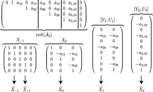
Figure 2: The reduced row-echelon form of $\dot{\mathcal{A}}_{\beta}$ contains all the information necessary to construct $V(\lambda)=[\Lambda(\widetilde{X}_{-1}),\dots,\Lambda(\widetilde{X}_{s-1})]$. An arrow from a column $[v;u]$ of $[Y_{k};U_{k}]$ indicates that the vector $\big{(}[\operatorname{rem}(\mathbb{X}_{k-1}u,p);v]+\operatorname{quo}(\iota(\mathbb{X}_{k-1}u),p)\big{)}$ is a column of $\widetilde{X}_{k}$.

Algorithm 2.

(Local Smith form, final version) $k=0$,   $R_{-1}=0$,   $\mathcal{A}_{0}=A^{(0)}$ $X_{0}=\mathbb{X}_{0}=\operatorname{null}(\dot{\mathcal{A}}_{0})$ $r_{0}=R_{0}=\operatorname{num\_cols}(\mathbb{X}_{0})$ (number of columns) $\widetilde{X}_{-1}=[e_{j_{1}},\dots,e_{j_{n-r_{0}}}]$, (columns $j_{i}$ of $\operatorname{rref}(\dot{\mathcal{A}}_{0})$ start new rows) while $R_{k}<\mu$ ($\mu$ = algebraic multiplicity of p) $k=k+1$ $\mathcal{A}_{k}=\big{[}\mathcal{A}_{k-1}\,,\,\operatorname{rem}(\big{[}A^{(k)},\dots,A^{(1)}\big{]}X_{k-1},p)+\operatorname{quo}(\big{[}A^{(k-1)},\dots,A^{(0)}\big{]}X_{k-1},p)\,\big{]}$ $\bullet$ $[Y_{k};U_{k}]=\text{ new columns of }\operatorname{null}(\dot{\mathcal{A}}_{k})$ beyond those of $\operatorname{null}(\dot{\mathcal{A}}_{k-1})$ $r_{k}=\operatorname{num\_cols}(U_{k})$, ($U_{k}$ is $R_{k-1}\times r_{k}$) $R_{k}=R_{k-1}+r_{k}$ $X_{k}=[\operatorname{rem}(\mathbb{X}_{k-1}U_{k},p);Y_{k}]+\operatorname{quo}(\iota(\mathbb{X}_{k-1}U_{k}),p)$ ($X_{k}$ is $n(k+1)\times r_{k}$) $\mathbb{X}_{k}=[\iota(\mathbb{X}_{k-1}),X_{k}]$ ($\mathbb{X}_{k}$ is $n(k+1)\times R_{k}$) $\widetilde{X}_{k-1}=X_{k-1}(:,[j_{1},\dots,j_{r_{k-1}-r_{k}}])$, (columns $n+R_{k-2}+j_{i}$ of end while $\operatorname{rref}(\dot{\mathcal{A}}_{k})$ start new rows) $\beta=k+1$ (maximal Jordan chain length) $\widetilde{X}_{\beta-1}=X_{\beta-1}$ $V(\lambda)=\big{[}\Lambda(\widetilde{X}_{-1}),\dots,\Lambda(\widetilde{X}_{\beta-1})\big{]}$

Figure 3: Algorithm for computing a unimodular local Smith form.

3.2 From Local to Global (Step 2)

Now that we have a local Smith form (22) for every irreducible factor $p_{j}(\lambda)$ of $\Delta(\lambda)$, we can use the extended Euclidean algorithm to obtain a family of polynomials $\{g_{j}(\lambda)\}_{j=1}^{l}$ with $\deg(g_{j}(\lambda))<s_{j}\kappa_{jn}$, where $s_{j}=\deg(p_{j})$, such that

$$\sum_{j=1}^{l}\bigg{[}g_{j}(\lambda)\prod_{k=1,k\neq j}^{l}p_{k}(\lambda)^{\kappa_{kn}}\bigg{]}=1,$$ (44)

where $p_{j}(\lambda)^{\kappa_{jn}}$ is the last entry in the diagonal matrix of the local Smith form at $p_{j}(\lambda)$. The integers $\kappa_{jn}$ are positive. We define a matrix polynomial $B_{n}(\lambda)$ via

$$B_{n}(\lambda)=\sum_{j=1}^{l}\bigg{[}g_{j}(\lambda)V_{j}(\lambda)\prod_{k\neq j}^{l}p_{k}(\lambda)^{\kappa_{kn}}\bigg{]}.$$ (45)

The main result of this section is stated as follows.

Proposition 12.

The matrix polynomial $B_{n}(\lambda)$ in (45) has two key properties:

1. Let ${b_{ni}}(\lambda)$ be the $i$th column of $B_{n}(\lambda)$. Then $A(\lambda){b_{ni}}(\lambda)$ is divisible by $d_{i}(\lambda)$, where $d_{i}(\lambda)=\prod_{j=1}^{l}p_{j}(\lambda)^{\kappa_{ji}}$ is the $i$th diagonal entry in $D(\lambda)$ of the Smith form.

2. $\det[B_{n}(\lambda)]$ is not divisible by $p_{j}(\lambda)$ for $j=1,\dots,l$.

Proof..

(1) Let $v_{ji}(\lambda)$ be the $i$th column of $V_{j}(\lambda)$. Then $A(\lambda)v_{ji}(\lambda)$ is divisible by $p_{j}(\lambda)^{\kappa_{ji}}$ and

$${b_{ni}}(\lambda)=\sum_{j=1}^{l}\bigg{[}\prod_{k\neq j}^{l}p_{k}(\lambda)^{\kappa_{kn}}\bigg{]}g_{j}(\lambda)v_{ji}(\lambda).$$

Since $\kappa_{jn}\geq\kappa_{ji}$ for $1\leq i\leq n$ and $1\leq j\leq l$, $A(\lambda){b_{ni}}(\lambda)$ is divisible by $d_{i}(\lambda)$.

(2) The local Smith form construction ensures that $p_{j}(\lambda)\nmid\det[V_{j}(\lambda)]$ for each $1\leq j\leq l$. Equation (44) modulo $p_{j}(\lambda)$ shows that $p_{j}(\lambda)\nmid g_{j}(\lambda)$. By definition,

$$\begin{split}\det[B_{n}(\lambda)]&=\det\big{(}\big{[}b_{n1}(\lambda)\,,\,\dots\,,\,b_{nn}(\lambda)\big{]}\big{)}=\det\big{(}\big{[}b_{ni}(\lambda)\big{]}_{i=1}^{n}\big{)}\\ &=\det\bigg{(}\bigg{[}\sum_{j^{\prime}=1}^{l}\bigg{(}\prod_{k\neq j^{\prime}}^{l}p_{k}(\lambda)^{\kappa_{kn}}\bigg{)}g_{j^{\prime}}(\lambda)v_{j^{\prime}i}(\lambda)\bigg{]}_{i=1}^{n}\bigg{)}.\end{split}$$

Each term in the sum is divisible by $p_{j}(\lambda)$ except $j^{\prime}=j$. Thus, by multi-linearity,

$$\operatorname{rem}(\det[B_{n}(\lambda)],p_{j}(\lambda))=\operatorname{rem}\Biggl{(}\bigg{[}\prod_{k\neq j}^{l}p_{k}(\lambda)^{\kappa_{kn}}\bigg{]}^{n}\big{[}g_{j}(\lambda)\big{]}^{n}\det\big{[}V_{j}(\lambda)\big{]},\,p_{j}(\lambda)\Biggr{)}\neq 0,$$

as claimed.    $\Box$

Remark 13.

It is possible for $\det[B_{n}(\lambda)]$ to be non-constant; however, its irreducible factors will be distinct from $p_{1}(\lambda),\dots,p_{l}(\lambda)$.

Remark 14.

Rather than building $B_{n}(\lambda)$ as a linear combination (45), we may form $B_{n}(\lambda)$ with columns

$$b_{ni}(\lambda)=\sum_{j=1}^{l}\bigg{[}\prod_{k\neq j}^{l}p_{k}(\lambda)^{\max(\kappa_{ki},1)}\bigg{]}g_{ij}(\lambda)v_{ji}(\lambda),\qquad(1\leq i\leq n),$$

where $\{g_{ij}\}_{j=1}^{l}$ solves the extended GCD problem

$$\sum_{j=1}^{l}\bigg{[}g_{ij}(\lambda)\prod_{k\neq j}^{l}p_{k}(\lambda)^{\max(\kappa_{ki},1)}\bigg{]}=1.$$

The two properties proved above also hold for this definition of $B_{n}(\lambda)$. This modification can significantly reduce the size of the coefficients in the computation when there is a wide range of Jordan chain lengths. But if $\kappa_{ji}$ only changes slightly for $1\leq i\leq n$, this change will not significantly affect the total running time of the algorithm.

3.3 Construction of Unimodular Multipliers (Step 3)

Given $[f_{1}(\lambda);\dots;f_{n}(\lambda)]\in K[\lambda]^{n}$, we can compute the Hermite form (20) to obtain a unimodular matrix $Q(\lambda)$ such that, after reversing rows, $Q(\lambda)f(\lambda)=[0;\dots;0;r(\lambda)]$, where $r=\gcd(f_{1},\dots,f_{n})$. We apply this procedure to the last column of $B_{n}(\lambda)$ and define $V_{n}(\lambda)=Q(\lambda)^{-1}$. The resulting matrix

$$B_{n-1}(\lambda):=V_{n}(\lambda)^{-1}B_{n}(\lambda)$$

is zero above the main diagonal in column $n$. We then apply this procedure to the first $n-1$ components of column $n-1$ of $B_{n-1}(\lambda)$ to get a new $Q(\lambda)$, and define

$$V_{n-1}(\lambda)=\left(\vbox{\hbox{\kern-1.15198pt\raise 0.0pt\hbox{\kern 43.6834pt}\kern 0.0pt\vbox{}\kern-1.15198pt}}\right).$$ (46)

It follows that $B_{n-2}(\lambda):=V_{n-1}(\lambda)^{-1}B_{n-1}(\lambda)$ is zero above the main diagonal in columns $n-1$ and $n$. Continuing in this fashion, we obtain unimodular matrices $V_{n}(\lambda)$, …, $V_{2}(\lambda)$ such that

$$A(\lambda)B_{n}(\lambda)=A(\lambda)\underbrace{V_{n}(\lambda)\cdots V_{2}(\lambda)}_{V(\lambda)}V_{2}(\lambda)^{-1}\cdots\underbrace{V_{n}(\lambda)^{-1}B_{n}(\lambda)}_{B_{n-1}(\lambda)}=A(\lambda)V(\lambda)B_{1}(\lambda),$$

where $V(\lambda)$ is unimodular, $B_{1}(\lambda)$ is lower triangular, and

$$\det[B_{1}(\lambda)]=\mathrm{const}\cdot\det[B_{n}(\lambda)].$$ (47)

The matrix $V(\lambda)$ puts $A(\lambda)$ in Smith form:

Proposition 15.

There is a unimodular matrix polynomial $E(\lambda)$ such that

$$A(\lambda)V(\lambda)=E(\lambda)D(\lambda),$$ (48)

where $D(\lambda)$ is of the form (3).

Proof..

Let $r_{mi}(\lambda)$ denote the entry of $B_{1}(\lambda)$ in the $m$th row and $i$th column. Define $y_{i}(\lambda)$ and $z_{i}(\lambda)$ to be the $i$th columns of $A(\lambda)V(\lambda)$ and $A(\lambda)V(\lambda)B_{1}(\lambda)$, respectively, so that

$$z_{i}(\lambda)=y_{i}(\lambda)r_{ii}(\lambda)+\sum_{m=i+1}^{n}y_{m}(\lambda)r_{mi}(\lambda),\qquad(1\leq i\leq n).$$ (49)

By Proposition 12, $z_{i}(\lambda)$ is divisible by $d_{i}(\lambda)$ for $1\leq i\leq n$ and $p_{j}(\lambda)\nmid\det[B_{1}(\lambda)]$ for $1\leq j\leq l$. It follows that the diagonal entries $r_{ii}(\lambda)$ of $B_{1}(\lambda)$ are relatively prime to each of the $d_{i}(\lambda)$. As $d_{n}(\lambda)$ divides $y_{n}(\lambda)r_{nn}(\lambda)$ and is relatively prime to $r_{nn}(\lambda)$, it divides $y_{n}(\lambda)$ alone. Now suppose $1\leq i<n$ and we have shown that $d_{m}(\lambda)$ divides $y_{m}(\lambda)$ for $i<m\leq n$. Then since $d_{i}(\lambda)$ divides $d_{m}(\lambda)$ for $m>i$ and $r_{ii}(\lambda)$ is relatively prime to $d_{i}(\lambda)$, we conclude from (49) that $d_{i}(\lambda)$ divides $y_{i}(\lambda)$. By induction, $d_{i}(\lambda)$ divides $y_{i}(\lambda)$ for $1\leq i\leq n$. Thus, there is a matrix polynomial $E(\lambda)$ such that (48) holds. Because $V(\lambda)$ is unimodular and $\det[A(\lambda)]=\operatorname{const}\cdot\det[D(\lambda)]$, it follows that $E(\lambda)$ is also unimodular, as claimed.    $\Box$

Remark 16.

$V(\lambda)$ constructed as described above puts $A(\lambda)$ in a global Smith form whether we build $B_{n}(\lambda)$ as a linear combination (45) or as in Remark 14.

Remark 17.

We can stop before reaching $V_{2}(\lambda)$ by adding a test

$$\textstyle\textbf{while }d_{k}\neq 1$$

to the loop in which $V(\lambda)$ is constructed. When the loop terminates, we have $V(\lambda)=V_{n}(\lambda)\cdots V_{k+1}(\lambda)$, where $k$ is the largest integer for which

$$d_{1}(\lambda)=\cdots=d_{k}(\lambda)=1.$$

Note that $k$ is known from the local Smith form calculations. The last $n-k$ columns of $V_{n}(\lambda)\cdots V_{k+1}(\lambda)$ are the same as those of $V_{n}(\lambda)\cdots V_{2}(\lambda)$; therefore, either can be used for $V(\lambda)$ as they contain identical Jordan chains.

Remark 18.

A slight modification of this procedure can significantly reduce the degree of the polynomials and the size of the coefficients in the computation. In this variant, rather than applying the extended GCD algorithm on $b_{nn}(\lambda)$ to find a unimodular matrix polynomial $Q(\lambda)$ so that $Q(\lambda)b_{nn}(\lambda)$ has the form $[0;\dots;0;r(\lambda)]$, we compute $Q(\lambda)$ that puts $\operatorname{rem}(b_{nn}(\lambda),d_{n}(\lambda))$ into this form. That is, we replace the last column of $B_{n}(\lambda)$ with $\operatorname{rem}(b_{nn}(\lambda),d_{n}(\lambda))$ before computing $Q(\lambda)$. To distinguish, we denote this new definition of $V_{n}(\lambda)=Q(\lambda)^{-1}$ by $\widetilde{V}_{n}(\lambda)$ and the resulting $B_{n-1}(\lambda)$ by $\widetilde{B}_{n-1}(\lambda)$. Continuing in this manner, we find unimodular matrix polynomials $\widetilde{V}_{n}(\lambda),\dots,\widetilde{V}_{k+1}(\lambda)$ by applying the procedure on $\operatorname{rem}(\tilde{b}_{ii}(\lambda),d_{i}(\lambda))$ for $i=n,\dots,k+1$, where $\tilde{b}_{ii}(\lambda)$ contains the first $i$ components of column $i$ of $\widetilde{B}_{i}(\lambda)$ and $k$ is defined as in Remark 17. We also define

$$\bar{B}_{i}=\widetilde{V}_{i+1}(\lambda)^{-1}\cdots\widetilde{V}_{n}(\lambda)^{-1}B_{n}(\lambda),\qquad(k\leq i\leq n-1).$$

Note that in general, $\bar{B}_{i}(\lambda)\neq\widetilde{B}_{i}(\lambda)$. It remains to show that this definition of $\widetilde{V}(\lambda)=\widetilde{V}_{n}(\lambda)\dots\widetilde{V}_{k+1}(\lambda)$, which satisfies

$$A(\lambda)B_{n}(\lambda)=A(\lambda)\underbrace{\widetilde{V}_{n}(\lambda)\cdots\widetilde{V}_{k+1}(\lambda)}_{\widetilde{V}(\lambda)}\widetilde{V}_{k+1}(\lambda)^{-1}\cdots\underbrace{\widetilde{V}_{n}(\lambda)^{-1}B_{n}(\lambda)}_{\bar{B}_{n-1}(\lambda)}=A(\lambda)\widetilde{V}(\lambda)\bar{B}_{k}(\lambda),$$

also puts $A(\lambda)$ in Smith form:

Proposition 19.

There is a unimodular matrix polynomial $\widetilde{E}(\lambda)$ such that

$$A(\lambda)\widetilde{V}(\lambda)=\widetilde{E}(\lambda)D(\lambda),$$ (50)

where $D(\lambda)$ is of the form (3).

Proof..

Define $\tilde{q}_{i}(\lambda)=\left[\operatorname{quo}(\tilde{b}_{ii}(\lambda),d_{i}(\lambda));0\right]\in M=R^{n}$ for $i=n,\dots,k+1$, where $0\in R^{n-i}$, $\tilde{b}_{ii}(\lambda)$ was defined above, and $\widetilde{B}_{n}(\lambda):=B_{n}(\lambda)$. Then we have

$$\begin{split}\widetilde{B}_{n-1}(\lambda)&=\widetilde{V}_{n}(\lambda)^{-1}\left(B_{n}(\lambda)-\left[\begin{array}[]{c|c}0_{n\times(n-1)}&d_{n}(\lambda)\tilde{q}_{n}(\lambda)\end{array}\right]\right)\\ &=\bar{B}_{n-1}(\lambda)-\left[\begin{array}[]{c|c}0_{n\times(n-1)}&d_{n}(\lambda)\widetilde{V}_{n}(\lambda)^{-1}\widetilde{q}_{n}(\lambda)\end{array}\right].\end{split}$$

The first $n-1$ columns of $\widetilde{B}_{n}(\lambda)$ are the same as those of $\bar{B}_{n}(\lambda)$. Continuing, we have

$$\begin{split}&\widetilde{B}_{n-2}(\lambda)=\widetilde{V}_{n-1}(\lambda)^{-1}\left(\widetilde{B}_{n-1}(\lambda)-\left[\begin{array}[]{c|c|c}0_{n\times(n-2)}&d_{n-1}(\lambda)\tilde{q}_{n-1}(\lambda)&0_{n\times 1}\end{array}\right]\right)\\ &\;\;=\widetilde{V}_{n-1}(\lambda)^{-1}\left(\bar{B}_{n-1}(\lambda)-\left[\begin{array}[]{c|c|c}0_{n\times(n-2)}&d_{n-1}(\lambda)\tilde{q}_{n-1}(\lambda)&d_{n}(\lambda)\widetilde{V}_{n}(\lambda)^{-1}\tilde{q}_{n}(\lambda)\end{array}\right]\right)\\ &\;\;=\bar{B}_{n-2}(\lambda)-\left[\begin{array}[]{c|c|c}0_{n\times(n-2)}&d_{n-1}(\lambda)\widetilde{V}_{n-1}(\lambda)^{-1}\tilde{q}_{n-1}(\lambda)&d_{n}(\lambda)\widetilde{V}_{n-1}(\lambda)^{-1}\widetilde{V}_{n}(\lambda)^{-1}\tilde{q}_{n}(\lambda)\end{array}\right].\end{split}$$

It follows by induction that

$$\widetilde{B}_{k}(\lambda)=\widetilde{V}_{k+1}(\lambda)^{-1}\left(\widetilde{B}_{k+1}(\lambda)-\left[\begin{array}[]{c|c|c}0_{n\times k}&d_{k+1}(\lambda)\tilde{q}_{k+1}(\lambda)&0_{n\times(n-k-1)}\end{array}\right]\right)$$ (52)

$$\;\;=\bar{B}_{k}(\lambda)-\left[\begin{array}[]{c|c|c|c}0_{n\times k}&d_{k+1}(\lambda)\widetilde{V}_{k+1}(\lambda)^{-1}\tilde{q}_{k+1}(\lambda)&\cdots&d_{n}(\lambda)\widetilde{V}_{k+1}(\lambda)^{-1}\cdots\widetilde{V}_{n}(\lambda)^{-1}\tilde{q}_{n}(\lambda)\end{array}\right].$$ (54)

$\widetilde{B}_{k}(\lambda)$ is zero above the main diagonal in columns $k+1$ to $n$. Define

$$u_{i}(\lambda):=\widetilde{V}_{k+1}(\lambda)^{-1}\cdots\widetilde{V}_{i}(\lambda)^{-1}\tilde{q}_{i}(\lambda),\qquad(k+1\leq i\leq n).$$

Then the $i$th column of the difference $\bar{B}_{k}(\lambda)-\widetilde{B}_{k}(\lambda)$ is $d_{i}(\lambda)u_{i}(\lambda)$ for $k+1\leq i\leq n$.

Let $\tilde{r}_{mi}(\lambda)$ denote the entry of $\widetilde{B}_{k}(\lambda)$ in the $m$th row and $i$th column. Define $\tilde{y}_{i}(\lambda)$ and $z_{i}(\lambda)$ to be the $i$th columns of $A(\lambda)\widetilde{V}(\lambda)$ and $A(\lambda)\widetilde{V}(\lambda)\bar{B}_{k}(\lambda)$, respectively, so that

$$z_{i}(\lambda)=\bigg{[}\tilde{y}_{i}(\lambda)\tilde{r}_{ii}(\lambda)+\sum_{m=i+1}^{n}\tilde{y}_{m}(\lambda)\tilde{r}_{mi}(\lambda)\bigg{]}+d_{i}(\lambda)A(\lambda)\widetilde{V}(\lambda)u_{i}(\lambda),\qquad(k+1\leq i\leq n).$$

By Proposition 12, $z_{i}(\lambda)$ is divisible by $d_{i}(\lambda)$ and $p_{j}(\lambda)\nmid\det[B_{n}(\lambda)]=\mathrm{const}\cdot\det[\bar{B}_{i-1}(\lambda)]$ for $k+1\leq i\leq n$ and $1\leq j\leq l$. As $d_{i}$ divides $d_{m}$ for $i\leq m\leq n$ and since (52) holds with $k$ replaced by $i-1$ for $k+1\leq i\leq n$, $\det[\bar{B}_{i-1}(\lambda)]-\det[\widetilde{B}_{i-1}(\lambda)]$ is divisible by $d_{i}(\lambda)$ due to multi-linearity of determinants. We also know that $\det[\widetilde{B}_{i-1}(\lambda)]$ is divisible by $\tilde{r}_{ii}(\lambda)$. Proof by contradiction shows that $\tilde{r}_{ii}(\lambda)$ is relatively prime to $d_{i}(\lambda)$ for $k+1\leq i\leq n$. Then we argue by induction as in the proof of Proposition 15 to conclude that $d_{i}(\lambda)$ divides $\tilde{y}_{i}(\lambda)$ for $k+1\leq i\leq n$. It holds trivially for $1\leq i\leq k$ as $d_{1}=\dots=d_{k}=1$. Thus, there is a matrix polynomial $\widetilde{E}(\lambda)$ such that (50) holds. Because $\widetilde{V}(\lambda)$ is unimodular and $\det[A(\lambda)]=\operatorname{const}\cdot\det[D(\lambda)]$, it follows that $\widetilde{E}(\lambda)$ is also unimodular.    $\Box$

4 Performance Comparison

In this section, we compare our algorithm to Villard’s method with good conditioning Villard95 , which is another deterministic sequential method for computing Smith forms with multipliers, and to ‘MatrixPolynomialAlgebra[SmithForm]’ in Maple. All three algorithms are implemented in exact arithmetic using Maple 13. The maximum number of digits that Maple can use for the numerator and denominator of a rational number (given by ‘kernelopts(maxdigits)’) is over 38 billion. However, limitations of available memory and running time set the limit on the largest integer number much lower than this. We use the variant of Algorithm 1 given in Appendix A to compute local Smith forms.

To evaluate the performance of these methods, we generate several groups of diagonal matrices $D(\lambda)$ over $\mathbb{Q}$ and multiply them on each side by unimodular matrices of the form $L(\lambda)Z(\lambda)$, where $L(\lambda)$ is unit lower triangular and $Z(\lambda)$ is unit upper triangular, both with off diagonal entries of the form $\lambda-i$ with $i\in\{-10,\dots,10\}$ a random integer. As a final step, we apply a row or column permutation to the resulting matrix. We find that row permutation has little effect on the running time of the algorithms while column permutation reduces the performance of Villard’s method. We compare the results in two extreme cases: (1) without column permutation and (2) with columns reversed. Each process is repeated five times for each $D(\lambda)$ and the median running time is recorded.

We use several parameters in the comparison, including the size $n$ of the square matrix $A(\lambda)$, the bound $d$ of the polynomial degrees of the entries in $A(\lambda)$, the number $l$ of irreducible factors in $\det[A(\lambda)]$, and the maximal Jordan chain length $\kappa_{jn}$.

In Figure 4, we show the running time of three tests with linear irreducible factors of the form $p_{j}=\lambda-\lambda_{j}$. As Villard’s method and Maple compute the left and right multipliers $U(\lambda)$ and $V(\lambda)$ while our algorithm instead computes $E(\lambda)$ and $V(\lambda)$, we also report the cost of inverting $E(\lambda)$ to obtain $U(\lambda)$ at the end of our algorithm (using Maple’s matrix inverse routine). This step could be made significantly faster by taking advantage of the fact that $E(\lambda)$ is unimodular. For example, one could store the sequence of elementary unimodular operations such that $T(\lambda)=Q_{m}(\lambda)\cdots Q_{1}(\lambda)E(\lambda)$ is unit upper triangular. It would not be necessary to actually form the matrices $T(\lambda)^{-1}$ or

$$U(\lambda)=T(\lambda)^{-1}Q_{m}(\lambda)\cdots Q_{1}(\lambda)$$ (55)

as the right hand side can be applied directly to any vector polynomial using back substitution to solve $T(\lambda)x(\lambda)=z(\lambda)$ in the last step. The same idea is standard in numerical linear algebra, where the $LU$-decomposition of a matrix is less expensive to compute than its inverse, and is equally useful. In the first test of Figure 4, $D_{n}(\lambda)$ is of the form

$$D_{n}(\lambda)=\operatorname{diag}[1,\dots,1,\lambda,\lambda(\lambda-1),\lambda^{2}(\lambda-1),\lambda^{2}(\lambda-1)^{2}],$$

where the matrix size $n$ increases, starting with $n=4$. Hence, we have $d=8$, $l=2$, and $\kappa_{1n}=\kappa_{2n}=2$ all fixed. (The unimodular matrices in the construction of $A(\lambda)$ each have degree 2.) For this test, inverting $E(\lambda)$ to obtain $U(\lambda)$ is the most expensive step of our algorithm. Without column permutation of the test matrices, our algorithm (with $U(\lambda)$) and Villard’s method have similar running times, both outperforming Maple’s built-in function. With column permutation, the performance of Villard’s method drops to the level of Maple’s routine while our algorithm remains faster.

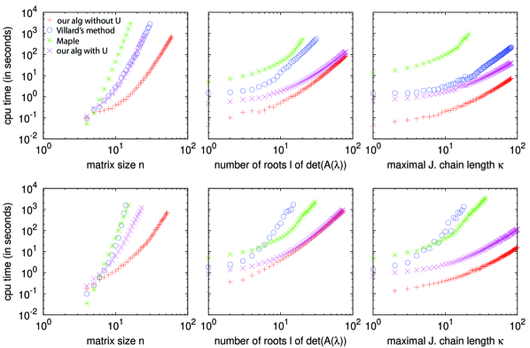
Figure 4: Comparison of running time of our algorithm (with or without computing $U(\lambda)$) to Villard’s method, and to Maple’s Smith form routine, on three families of test matrices. (Top row) without column permutation of test matrices. (Bottom row) with column permutation.

For the second test, we use test matrices $D_{l}(\lambda)$ of size $9\times 9$, where $l$ is the number of roots of $\det[A(\lambda)]$:

$$D_{l}(\lambda)=\operatorname{diag}[1,\dots,1,\prod_{j=1}^{l}(\lambda-j)],\qquad(l=1,2,\dots).$$

Thus, $n=9$, $d=l+4$ and $\kappa_{jn}=1$ for $1\leq j\leq l$. This time the relative cost of inverting $E(\lambda)$ to obtain $U(\lambda)$ decreases with $l$ in our algorithm, which is significantly faster than the other two methods whether or not we permute columns in the test matrices. In the third test, we use $9\times 9$ test matrices $D_{k}(\lambda)$ of the form

$$D_{k}(\lambda)=\operatorname{diag}[1,\dots,1,(\lambda-1)^{k}],\qquad(k=1,2,\dots),$$

with $n=9$, $l=1$, $\kappa_{1n}=k$ and $d=k+4$. We did not implement the re-use strategy for computing the reduced row-echelon form of $\mathcal{A}_{k}$ by storing the Gauss-Jordan transformations used to obtain $\operatorname{rref}(\mathcal{A}_{k-1})$, and then continuing with only the new columns of $\mathcal{A}_{k}$. This is because the built-in function LinearAlgebra[ReducedRowEchelonForm] is much faster than can be achieved by a user defined Maple code for the same purpose. In a lower level language (or with access to Maple’s internal code), this re-use strategy would decrease the running time of local Smith form calculations in this test from $O(k^{4})$ to $O(k^{3})$. A similar decrease in the cost of computing the left-multiplier $U(\lambda)=E(\lambda)^{-1}$ could be achieved by computing $T(\lambda)$ in (55) instead.

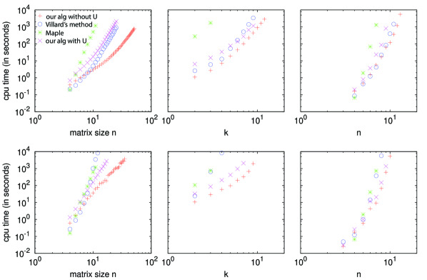
Figure 5: Comparison of running times of the algorithms for three test problems in which the irreducible factors $p_{j}(\lambda)$ of the determinant are of degree greater than 1. (Top row) without column permutation of test matrices. (Bottom row) with column permutation.

We also evaluate the performance on three test problems (numbered 4–6) with irreducible polynomials of higher degree. The results are given in Figure 5. In the fourth test, we use matrices $D_{n}(\lambda)$ similar to those in the first test, but with irreducible polynomials of degree $2$ and $4$. Specifically, we define

$$D_{n}(\lambda)=\operatorname{diag}[1,\dots,1,p_{1},p_{1}p_{2},p_{1}^{2}p_{2},p_{1}^{2}p_{2}^{2}],\qquad(n=4,5,\dots),$$

where $p_{1}=\lambda^{2}+\lambda+1$, $p_{2}=\lambda^{4}+\lambda^{3}+\lambda^{2}+1$, $\kappa_{1n}=2$, $\kappa_{2n}=2$, and $d=16$. When the columns of the test matrices are permuted, our algorithm is faster than the other two methods whether or not $U(\lambda)$ is computed. When the columns are not permuted, computing $U(\lambda)$ causes our method to be slower than Villard’s method. In this test, our algorithm would benefit from switching to the $R/pR$ version of Algorithm 2 rather than the version over $K$ described in the appendix. It would also benefit from computing $T(\lambda)$ in (55) rather than the full inverse $U(\lambda)=E(\lambda)^{-1}$. In the fifth test, we use $9\times 9$ test matrices $D_{k}(\lambda)$ of the form

$$D_{k}(\lambda)=\operatorname{diag}[1,\dots,1,\prod_{j=1}^{k}(\lambda^{2}+j),\prod_{j=1}^{k}(\lambda^{2}+j)^{2},\prod_{j=1}^{k}(\lambda^{2}+j)^{k}],\qquad(k=2,3,\dots),$$

with $n=9$, $l=k$, $\kappa_{jn}=k$ and $d=2k^{2}+4$. Both the number of factors and maximal Jordan chain length increase with $k$. Our algorithm performs much better than the others when column permutations are performed on the test matrices. In the final test, we define $n\times n$ matrices

$$D_{n}(\lambda)=\operatorname{diag}[1,1,(\lambda^{2}+1),(\lambda^{2}+1)^{2}(\lambda^{2}+2),\dots,\prod_{j=1}^{n-2}(\lambda^{2}+j)^{n-1-j}],\qquad(n=3,4,\dots)$$

so that all the parameters $n$, $l=n-2$, $\kappa_{jn}=n-1-j$ and $d=(n-1)(n-2)+4$ increase simultaneously. All three algorithms run very slowly on this last family of test problems.

5 Discussion

The key idea of our algorithm is that it is much less expensive to compute local Smith forms through a sequence of nullspace calculations than it is to compute global Smith forms through a sequence of unimodular row and column operations. This is because (1) row reduction over $R/pR$ in Algorithm 2 (or over $K$ in Appendix A) is less expensive than computing Bézout coefficients over $R$; (2) the size of the rational numbers that occur in the algorithm remain smaller (as we only deal with the leading terms of $A$ in an expansion in powers of $p$ rather than with all of $A$); and (3) each column of $V(\lambda)$ in a local Smith form only has to be processed once for each power of $p$ in the corresponding diagonal entry of $D(\lambda)$. Once the local Smith forms are known, we combine them to form a (global) multiplier $V(\lambda)$ for $A(\lambda)$. This last step does involve triangularization of $B_{n}(\lambda)$ via the extended GCD algorithm, but this is less time consuming in most cases than performing unimodular row and column operations on $A(\lambda)$ to obtain $D(\lambda)$. This is because we only have to apply row operations to $B_{n}(\lambda)$ (as the columns are already correctly ordered); we keep the degree of polynomials (and therefore the number of terms) in the algorithm small with the operation $\operatorname{rem}(\cdot,d_{i})$; and the leading columns of $B_{n}(\lambda)$ tend to be sparse (as they consist of a superposition of local Smith forms, whose initial columns $X_{-1}$ are a subset of the columns of the identity matrix). Sparsity is not used explicitly in our code, but it does reduce the work required to compute the Bézout coefficients of a column.

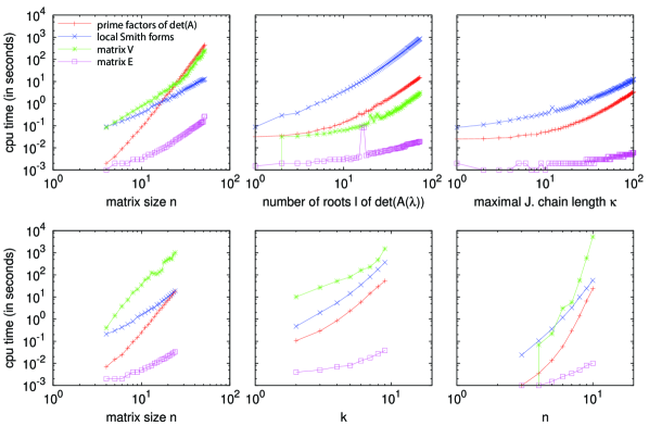
Figure 6: Running time of each step of our algorithm for the six test problems of Section 4.

A detailed breakdown of the running time of each step of our algorithm is given in Figure 6. For each test in Section 4, we show only the case where columns of the test matrices are permuted; the other case is similar. The step labeled “prime factors of $\operatorname{det}(A)$” shows the time of computing the determinant and factoring it into prime factors. The step labeled “local Smith forms” could be made faster in tests 4–6 by working over $R/pR$ (using Algorithm 2 rather than the variant in the appendix) as the irreducible factors $p_{j}(\lambda)$ have degree $s_{j}>1$ in these tests. Also, although it is not implemented in this paper, this local Smith form construction would be easy to parallelize. The step labeled “matrix $V$” reports the time of computing $V(\lambda)$ from $B_{n}(\lambda)$. The cost of this step is zero when there is only one irreducible factor in $\det[A(\lambda)]$ as $B_{n}(\lambda)$ is already unimodular in that case. This happens when $l=1$ in the second test, in all cases in the third test, and when $n=3$ in the last test. Finally, the step labeled “matrix $E$” reports the time of computing $E(\lambda)=A(\lambda)V(\lambda)D(\lambda)^{-1}$.

The obvious drawback of our algorithm is that we have to compute a local Smith form for each irreducible factor of $\Delta(\lambda)$ separately, while much of the work in deciding whether to accept a column in Algorithm 1 can be done for all the irreducible factors simultaneously by using extended GCDs. In our numerical experiments, it appears that in most cases, the benefit of computing local Smith forms outweighs the fact that there are several of them to compute.

Appendix A Alternative Version of Algorithm 2

In this section we present an algebraic framework for local Smith forms of matrix polynomials that shows the connection between Algorithm 2 and the construction of canonical systems of Jordan chains presented in Wilken2007 . This leads to a variant of the algorithm in which row-reduction is done in the field $K$ rather than in $R/pR$.

Suppose $R$ is a principal ideal domain and $p$ is a prime in $R$. $M$ defined via $M=R^{n}$ is a free $R$-module with a free basis $\{(1,0,\dots,0),\dots,(0,\dots,1)\}$. Suppose $A:M\to M$ is a $R$-module morphism. We define submodules

$$N_{k}=\big{\{}x\in M:Ax\text{ is divisible by }p^{k}\big{\}},\qquad(k\geq 0).$$ (56)

Then $N_{k}$ is a free submodule of $M$ by the structure theorem hungerford for finitely generated modules over a principal ideal domain. (The structure theorem states that if $M$ is a free module over a principal ideal domain $R$, then every submodule of $M$ is free.) The rank of $N_{k}$ is also $n$, as $p^{k}M\subset N_{k}\subset M$. Note that $N_{0}=M$ and

$$N_{k+1} \subset N_{k}, (k\geq 0),$$ (57)

$$N_{k+1}\cap pM =pN_{k}, (k\geq 0).$$ (58)

Next we define the spaces $W_{k}$ via

$$W_{k}=N_{k+1}/pN_{k},\qquad(k\geq-1),$$ (59)

where $N_{-1}:=M$ so that $W_{-1}=M/pM$. By (58), the action of $R/pR$ on $W_{k}$ is well-defined, i.e. $W_{k}$ is a vector space over this field. Let us denote the canonical projection $M\rightarrow M/pM$ by $\pi$. Note that $\pi(pN_{k})=0$, so $\pi$ is well-defined from $W_{k}$ to $M/pM$ for $k\geq-1$. It is also injective as $xp\in N_{k+1}\Rightarrow x\in N_{k}$, by (58). Thus, cosets $\{\dot{x}_{1},\dots,\dot{x}_{m}\}$ are linearly independent in $W_{k}$ iff $\{\pi(x_{1}),\dots,\pi(x_{m})\}$ are linearly independent in $M/pM$. We define the integers

$$r_{k}=\text{dimension of $W_{k}$ over $R/pR$},\qquad(k\geq-1)$$ (60)

and note that $r_{-1}=n$ and $r_{k}>0$ iff there exists $x\in M$ such that $p\nmid x$ and $p^{k+1}\mid Ax$. We also observe that the truncation operator

$$id:W_{k+1}\rightarrow W_{k}:(x+pN_{k+1})\mapsto(x+pN_{k}),\qquad(k\geq-1)$$ (61)

is well-defined ($pN_{k+1}\subset pN_{k}$) and injective ($x\in N_{k+2}$ and $x\in pN_{k}$ $\Rightarrow$ $x\in pN_{k+1}$, due to (58)). We may therefore consider $W_{k+1}$ to be a subspace of $W_{k}$ for $k\geq-1$, and have the inequalities

$$r_{k+1}\leq r_{k},\qquad(k\geq-1).$$ (62)

The case $r_{0}=0$ is not interesting (as $N_{k}=p^{k}M$ for $k\geq 0$), so we assume that $r_{0}>0$. Lemma 8 shows that when $R=K[\lambda]$, which we assume from now on, $r_{0}>0$ is equivalent to the condition that $\det[A(\lambda)]$ is divisible by $p(\lambda)$. We also assume that $r_{k}$ eventually decreases to zero, say

$$r_{k}=0\quad\Leftrightarrow\quad k\geq\beta,\qquad\beta:=\text{maximal Jordan chain length}.$$ (63)

This follows from the assumption that $\det[A(\lambda)]$ is not identically zero. It will be useful to define the index sets $I_{k}=\{i\;:\;n-r_{k-1}+1\leq i\leq n-r_{k}\}$ for $k=0,\dots,\beta$.

Any matrix $V=[x_{1},\dots,x_{n}]$ will yield a local Smith form $AV=ED$ provided that $x_{i}\in N_{k}$ for $i\in I_{k}$ ($0\leq k\leq\beta$) and the vectors

$$\{x_{i}+pN_{k-1}\}_{i\in I_{k}}$$ (64)

form a basis for any complement $\widetilde{W}_{k-1}$ of $W_{k}$ in $W_{k-1}$. To see that $p\nmid\det E$, we use induction on $k$ to show that the vectors

$$\{\operatorname{quo}(Ax_{i},p^{\alpha_{i}})+pM\}_{i=1}^{n-r_{k}}$$ (65)

are linearly independent in $M/pM$, where

$$\alpha_{i}=k,\qquad(i\in I_{k}).$$ (66)

Otherwise, a linear combination of the form $\star$ in Algorithm 1 would exist that belongs to $\widetilde{W}_{k-1}\cap W_{k}$, a contradiction. The result that $p\nmid\det E$ follows from Lemma 8. The while loop in Algorithm 1 is a systematic procedure for computing such a collection $\{x_{i}\}_{i\in I_{k}}$, and has the added benefit of yielding a unimodular multiplier $V$.

We now wish to find a convenient representation for these spaces suitable for computation. Since $p^{k+1}M\subset pN_{k}$, we have the $R$-module isomorphism

$$N_{k+1}/pN_{k}\cong(N_{k+1}/p^{k+1}M)/(pN_{k}/p^{k+1}M),$$ (67)

i.e.

$$W_{k}\cong\mathbb{W}_{k}/p\mathbb{W}_{k-1},\quad(k\geq 0),\qquad\mathbb{W}_{k}:=N_{k+1}/p^{k+1}M,\quad(k\geq-1).$$ (68)

Although the quotient $\mathbb{W}_{k}/p\mathbb{W}_{k-1}$ is a vector space over $R/pR$, the spaces $\mathbb{W}_{k}$ and $M/p^{k+1}M$ are not. They are, however, modules over $R/p^{k+1}R$ and vector spaces over $K$. Note that $A(\lambda)$ induces a linear operator $\mathbb{A}_{k}$ on $M/p^{k+1}M$ with kernel

$$\mathbb{W}_{k}=\ker\mathbb{A}_{k},\qquad(k\geq-1).$$ (69)

We also define

$$R_{k}=\frac{\text{dimension of $\mathbb{W}_{k}$ over }K}{s},\qquad(k\geq-1,\quad s=\deg p)$$ (70)

so that $R_{-1}=0$ and

$$R_{k}=r_{0}+\cdots+r_{k},\qquad(k\geq 0),$$ (71)

where we used $\mathbb{W}_{0}=W_{0}$ together with (68) and the fact that as a vector space over $K$, $\dim W_{k}=sr_{k}$. By (66), $r_{k-1}-r_{k}=\#\{i\;:\;\alpha_{i}=k\}$, so

$$R_{\beta-1} =r_{0}+\cdots+r_{\beta-1}=(r_{-1}-r_{0})0+(r_{0}-r_{1})1+\cdots+(r_{\beta-1}-r_{\beta})\beta$$ (72)

$$=\alpha_{1}+\cdots+\alpha_{n}=\mu=\text{algebraic multiplicity of $p$},$$

where we used Theorem 7 in the last step. We also note that $\nu:=R_{0}=s^{-1}\dim\ker(\mathbb{A}_{0})$ can be interpreted as the geometric multiplicity of $p$.

Equations (68) and (69) reduce the problem of computing Jordan chains to that of finding kernels of the linear operators $\mathbb{A}_{k}$ over $K$. If we represent elements $x\in M/p^{k+1}M$ as lists of coefficients $x^{(j,l,m)}\in K$ such that the components of $x$ involve the terms

$$x^{(j,l,m)}p^{j}\lambda^{m},\qquad 0\leq j\leq k,\quad 1\leq l\leq n,\quad 0\leq m\leq s-1,$$ (73)

then multiplication by $\lambda$ in $M/p^{k+1}M$ becomes the following linear operator on $K^{sn(k+1)}$:

$$\mathbb{S}_{k}=\begin{pmatrix}I\otimes S&0&0&0\\[1.0pt] I\otimes Z&I\otimes S&0&0\\[-4.0pt] 0&\ddots&\ddots&0\\[1.0pt] 0&0&I\otimes Z&I\otimes S\end{pmatrix}\!,\qquad S\text{ as in (\ref{eq_S_def})},\qquad Z=\begin{pmatrix}0&0&1\\[-4.0pt] &\ddots&0\\[2.0pt] 0&&0\end{pmatrix}\!.$$ (74)

Here $\mathbb{S}_{k}$ is a $(k+1)\times(k+1)$ block matrix, $I\otimes S$ is a Kronecker product of matrices, $S$ and $Z$ are $s\times s$ matrices, and $I$ is $n\times n$. Multiplication by $\lambda^{m}$ is represented by $\mathbb{S}_{k}^{m}$, which has a similar block-Toeplitz structure to $\mathbb{S}_{k}$ for $2\leq m\leq s-1$, but with $S$ replaced by $S^{m}$ and $Z$ replaced by

$$Z_{m}=\begin{cases}0&\quad m=0\\ \sum_{l=0}^{m-1}S^{l}ZS^{m-1-l},&1\leq m\leq s-1.\end{cases}$$ (75)

The matrix $p(\mathbb{S}_{k})^{j}$ is a shift operator with identity blocks $I_{n}\otimes I_{s}$ on the $j$th sub-diagonal. If we expand

$$A(\lambda)=A^{(0)}+pA^{(1)}+\cdots+p^{q}A^{(q)},\qquad A^{(j)}=A^{(j,0)}+\cdots+\lambda^{s-1}A^{(j,s-1)},$$ (76)

the matrix $\mathbb{A}_{k}$ representing $A(\lambda)$ is given by

$$\mathbb{A}_{k}=\left(\begin{array}[]{cccc}A_{0}&0&\cdots&0\\ A_{1}&A_{0}&\cdots&0\\ \cdots&\cdots&\cdots&\cdots\\ A_{k}&A_{k-1}&\cdots&A_{0}\end{array}\right),$$ (77)

where

$$A_{j}=\begin{cases}\sum_{m=0}^{s-1}A^{(0,m)}\otimes S^{m},&\quad j=0,\\ \sum_{m=0}^{s-1}\big{[}A^{(j,m)}\otimes S^{m}+A^{(j-1,m)}\otimes Z_{m}\big{]},&\quad j\geq 1.\end{cases}$$ (78)

This formula may be derived by observing that the matrix representation of the action of $p(\lambda)^{j}\lambda^{m}A^{(j,m)}$ on $M/p^{k+1}M$ is block Toeplitz with $A^{(j,m)}\otimes S^{m}$ on the $j$th sub-diagonal and $A^{(j,m)}\otimes Z_{m}$ on the $(j+1)$st. Defining $A_{j}$ this way avoids the need to compute remainders and quotients in subsequent steps (such as occur in Algorithm 2).

Next we seek an efficient method of computing a basis matrix $\mathbb{X}_{k}$ for the nullspace $\mathbb{W}_{k}=\ker\mathbb{A}_{k}$. Suppose $k\geq 1$ and we have computed $\mathbb{X}_{k-1}$. The first $k$ blocks of equations in $\mathbb{A}_{k}\mathbb{X}_{k}=0$ imply there are matrices $\mathbb{U}_{k}$ and $\mathbb{Y}_{k}$ such that $\mathbb{X}_{k}=[\mathbb{X}_{k-1}\mathbb{U}_{k};\mathbb{Y}_{k}]$, while the last block of equations is

$$\overbrace{\left(\begin{array}[]{cccc}A_{k}&\dots&A_{0}\end{array}\right)\left(\begin{array}[]{cc}0&\mathbb{X}_{k-1}\\ I_{sn\times sn}&0\\ \end{array}\right)}^{\mathcal{A}_{k}}\underbrace{\phantom{\left(\begin{array}[]{cc}0&\mathbb{X}_{k-1}\\ I_{sn\times sn}&\mathbb{B}_{k-1}\\ \end{array}\right)}\left(\begin{array}[]{c}\mathbb{Y}_{k}\\ \mathbb{U}_{k}\\ \end{array}\right)}_{\mathbb{X}_{k}}=\left(\begin{array}[]{c}0_{sn\times sR_{k}}\end{array}\right).$$ (79)

The matrices $\mathbb{X}_{k}$ can be built up recursively by setting $X_{0}=\mathbb{X}_{0}=\mathbb{Y}_{0}=\operatorname{null}(A_{0})$, defining $\mathbb{U}_{0}$ to be an empty matrix (with zero rows and $sR_{0}$ columns), and computing

$$\mathcal{A}_{k}=\Big{(}\mathcal{A}_{k-1}\,,\,[A_{k},\dots,A_{1}]X_{k-1}\Big{)},\qquad(k\geq 1)$$

$$[Y_{k};U_{k}]=\text{new columns of }\operatorname{null}(\mathcal{A}_{k})\text{ beyond those of }\operatorname{null}(\mathcal{A}_{k-1}),$$

$$[\mathbb{Y}_{k};\mathbb{U}_{k}]=\begin{pmatrix}\mathbb{Y}_{k-1}&Y_{k}\\ [\mathbb{U}_{k-1};0]&U_{k}\end{pmatrix},\qquad\begin{aligned} X_{k}&=[\mathbb{X}_{k-1}U_{k};Y_{k}],\\[2.0pt] \mathbb{X}_{k}&=[\iota(\mathbb{X}_{k-1}),X_{k}].\end{aligned}$$

Here $\iota:K^{snl}\rightarrow K^{sn(l+1)}$ represents multiplication by $p$ from $M/p^{l}M$ to $M/p^{l+1}M$:

$$\iota([x^{(0)};\dots;x^{(l-1)}])=[0;x^{(0)};\dots;x^{(l-1)}],\qquad x^{(j)},\,0\in K^{sn}.$$ (80)

By construction, $\mathbb{X}_{k}=[\iota(\mathbb{X}_{k-1}),X_{k}]$ is a basis for $\mathbb{W}_{k}$ when $k\geq 1$; it follows that $X_{k}+\iota(\mathbb{W}_{k-1})$ is a basis for $W_{k}$ when $W_{k}$ is viewed as a vector space over $K$. We define $X_{0}=\mathbb{X}_{0}$ and $X_{-1}=I_{sn\times sn}$ to obtain bases for $W_{0}$ and $W_{-1}$ as well.

But we actually want a basis for $W_{k}$ viewed as a vector space over $R/pR$ rather than $K$. Fortunately, all the matrices in this construction are manipulated $s\times s$ blocks, and the desired basis over $R/pR$ may be obtained by selecting the first column from each supercolumn (group of $s$ columns) of $X_{k}$. Indeed, if $[x_{1},\dots,x_{s}]$ is a supercolumn of $X_{k}$, we are able to prove that $x_{j}-\mathbb{S}_{k}x_{j-1}\in\iota(\mathbb{W}_{k-1})$ for $2\leq j\leq s$. Since $\mathbb{S}_{k}$ represents multiplication by $\lambda$, these columns are all equivalent over $R/pR$. We are also able to prove that constructing $X_{k}$ in this way (using the first column of each supercolumn) is equivalent to Algorithm 2, i.e. it yields the same unimodular matrix $V(\lambda)$ that puts $A(\lambda)$ in local Smith form. We omit the proof as it is long and technical, involving a careful comparison of nullspace calculations via row-reduction in the two algorithms.

In practice, this version of the algorithm (over $K$) is easier to implement, but the other version (over $R/pR$) should be about $s$ times faster as the cost of multiplying two elements of $R/pR$ is $O(s^{2})$ while the cost of multiplying two $s\times s$ matrices is $O(s^{3})$. The results in Section 4 were computed as described in this appendix (over $K=\mathbb{Q}$).

References

- [1] K. E. Avrachenkov, M. Haviv, and P. G. Howlett. Inversion of analytic matrix functions that are singular at the origin. SIAM J. Matrix Anal. Appl., 22(4):1175–1189, 2001.
- [2] T. H. Cormen, C. E. Leiserson, R. L. Rivest, and C. Stein. Introduction to Algorithms. MIT Press, Cambridge, MA, 2001.
- [3] James W. Demmel. Applied Numerical Linear Algebra. SIAM, Philadelphia, 1997.
- [4] A. Edelman, E. Elmroth, and B. Kågström. A geometric approach to perturbation theory of matrices and matrix pencils, part I: versal deformations. SIAM J. Matrix Anal. Appl., 18(3):653–692, 1997.
- [5] F.R. Gantmacher. Matrix Theory, volume 1. Chelsea Publishing Company, 1960.
- [6] I. Gohberg, M. A. Kaashoek, and F. van Schagen. On the local theory of regular analytic matrix functions. Linear Algebra Appl., 182:9–25, 1993.
- [7] I. Gohberg, P. Lancaster, and L. Rodman. Matrix Polynomials. Academic Press, New York, 1982.
- [8] Gene H. Golub and Charles F. Van Loan. Matrix Computations. John Hopkins University Press, Baltimore, 1996.
- [9] Thomas W. Hungerford. Algebra. Springer, New York, 1996.
- [10] T. Kailath. Linear Systems. Prentice Hall, Englewood Cliffs, 1980.
- [11] E. Kaltofen, M.S. Krishnamoorthy, and B.D. Saunders. Fast parallel computation of Hermite and Smith forms of polynomial matrices. SIAM J. Alg. Disc. Meth., 8(4):683–690, 1987.
- [12] E. Kaltofen, M.S. Krishnamoorthy, and B.D. Saunders. Parallel algorithms for matrix normal forms. Linear Algebra and its Applications, 136:189–208, 1990.
- [13] R. Kannan. Solving systems of linear equations over polynomials. Theoretical Computer Science, 39:69–88, 1985.
- [14] S. Labhalla, H. Lombardi, and R. Marlin. Algorithmes de calcul de la r duction de hermite d’une matrice coefficients polynomiaux. Theoretical Computer Science, 161:69–92, 1996.
- [15] W. H. Neven and C. Praagman. Column reduction of polynomial matrices. Linear Algebra Appl., 188:569–589, 1993.
- [16] H. H. Rosenbrock. State-space and Multivariable Theory. Wiley, New York, 1970.
- [17] A. Storjohann. Computation of Hermite and Smith normal forms of matrices. Master’s thesis, Dept. of Computer Science, Univ. of Waterloo, Canada, 1994.
- [18] A. Storjohann and G. Labahn. A fast las vegas algorithm for computing the Smith normal form of a polynomial matrix. Linear Algebra and its Applications, 253:155–173, 1997.
- [19] P. Van Dooren. The computation of Kronecker’s canonical form of a singular pencil. Linear Algebra Appl., 27:103–140, 1979.
- [20] P. Van Dooren and P. Dewilde. The eigenstructure of an arbitrary polynomial matrix: computational aspects. Linear Algebra Appl., 50:545–579, 1983.
- [21] G. Villard. Computation of the Smith normal form of polynomial matrices. In International Symposium on Symbolic and Algebraic Computation, Kiev, Ukraine, pages 209–217. ACM Press, 1993.
- [22] G. Villard. Fast parallel computation of the Smith normal form of polynomial matrices. In International Symposium on Symbolic and Algebraic Computation, Oxford, UK, pages 312–317. ACM Press, 1994.
- [23] G. Villard. Generalized subresultants for computing the Smith normal form of polynomial matrices. J. Symbolic Computation, 20:269–286, 1995.
- [24] G. Villard. Fast parallel algorithms for matrix reduction to normal forms. Appli. Alg. Eng. Comm. Comp., 8(6):511–538, 1997.
- [25] J. Wilkening. An algorithm for computing Jordan chains and inverting analytic matrix functions. Linear Algebra Appl., 427/1:6–25, 2007.
- [26] J. C. Zúñiga Anaya and D. Henrion. An improved Toeplitz algorithm for polynomial matrix null-space computation. Appl. Math. Comput., 207:256–272, 2009.