Binary frequency of very young brown dwarfs
at separations smaller than 3 AU

Searches for companions of brown dwarfs by direct imaging mainly probe orbital separations greater than 3–10 AU. On the other hand, previous radial velocity surveys of brown dwarfs are mainly sensitive to separations smaller than 0.6 AU. It has been speculated that the peak of the separation distribution of brown dwarf binaries lies right in the unprobed range. This work extends high-precision radial velocity surveys of brown dwarfs for the first time out to 3 AU. Based on more than six years UVES/VLT spectroscopy the binary frequency of brown dwarfs and (very) low-mass stars (M4.25-M8) in Chamaeleon I was determined: 18${}^{+20}_{-12}$ % for the whole sample and 10${}^{+18}_{-8}$ % for the subsample of ten brown dwarfs and very low-mass stars (M$\lesssim 0.1\,M_{\odot}$). Two spectroscopic binaries were confirmed, the brown dwarf candidate Cha H$\alpha$ 8 (previously discovered by Joergens & Müller) and the low-mass star CHXR 74. Since their orbital separations appear to be 1 AU or greater, the binary frequency at $<$1 AU might be less than 10%. Now for the first time companion searches of (young) brown dwarfs cover the whole orbital separation range, and the following observational constraints for models of brown dwarf formation can be derived: (i) the frequency of brown dwarf and very low-mass stellar binaries at $<$3 AU does not significantly exceed that at $>$3 AU; i.e. direct imaging surveys do not miss a significant fraction of brown dwarf binaries; (ii) the overall binary frequency of brown dwarfs and very low-mass stars is 10-30 %; (iii) the decline in the separation distribution of brown dwarfs towards smaller separations seems to occur between 1 and 3 AU; (iv) the observed continuous decrease in the binary frequency from the stellar to the substellar regime is confirmed at $<$3 AU providing further evidence of a continuous formation mechanism from low-mass stars to brown dwarfs.

1 Introduction

Searching for companions to brown dwarfs (BDs) is essential for understanding BD formation, for which no widely accepted model exits (e.g. recent review by Luhman et al. 2007). A priori, one might expect that BDs form in the same manner as stars by the direct collapse and fragmentation of molecular clouds, only on a much smaller scale. Standard cloud fragmentation seems to have difficulty in making BDs (Boss 2001; Bate, Bonnell & Bromm 2003). One possible explanation is that the simulations lack an important piece of physics; e.g., supersonic magneto-turbulence can create local high densities and facilitate the formation of BDs (Padoan & Nordlund 2004). Alternatively, BDs are formed when cloud fragmentation is modified by an additional process that prematurely halts accretion during the protostellar stage, such as dynamical ejection out of the dense gaseous environment (e.g. Reipurth & Clarke 2001; Boss 2001; Bate, Bonnell & Bromm 2002; Sterzik & Durisen 2003; Umbreit et al. 2005) or photoevaporation by ionizing radiation from nearby massive stars (Kroupa & Bouvier 2003; Whitworth & Zinnecker 2004). A fourth, recently studied scenario foresees BD formation through instabilities in the outer ($\gtrsim$100 AU) disk around a star and release into the field by e.g. secular perturbation (Goodwin & Whitworth 2007; Stamatellos et al. 2007).

The frequency and properties of BDs in multiple systems are fundamental parameters in these models, e.g. embryo-ejection scenarios for BD formation predict only a few BD binaries in preferentially close orbits, while isolated fragmentation scenarios are expected to generate BD binaries with similar (scaled-down) properties, as stellar binaries have. However, the binary properties of BDs are poorly constrained for close separations. Most of the current surveys for companions to BDs and very low-mass stars (VLMS, $M\leq 0.1\,M_{\odot}$) are done by direct (adaptive optics or HST) imaging (e.g. Reid et al. 2001; Bouy et al. 2003; Burgasser et al. 2003; Gizis et al. 2003; Close et al. 2003; see also Burgasser et al. 2007) and are not sensitive to either close separations ($a\lesssim 2$–3 AU and $a\lesssim 10$–15 AU for the field and clusters, respectively) nor to low-mass ratio systems (q$\equiv$M₂/M${}_{1}\lesssim$0.6). These surveys find a lower frequency (10-30%) of BD/VLM binaries compared to stars, a separation distribution with a peak around 3–10 AU, and a preference for equal-mass components with 77% having a mass ratio q$\geq$0.8. The observed peak of the separation distribution is close to the incompleteness limit; thus, we do not know if there is a significant number of still undetected, very close ($<$3 AU) BD/VLM binaries. It has been suggested that BD/VLM binaries with a separation $<$3 AU are as frequent or even more frequent than those at $>$3 AU (Pinfield et al 2003; Maxted & Jeffries 2005; Burgasser et al. 2007). Hence, the peak of the BD/VLM binary separation distribution could lie below 3 AU. Furthermore, while it has been argued that the higher frequency of systems with mass ratios close to unity appears to be a real feature of very low-mass binaries, it would be, nevertheless, desirable to actually probe mass ratios lower than 0.6. Given these limits to the current observational data, the question arises as to whether our current picture of BD/VLM binaries is complete, or, whether we miss a significant fraction of very close and/or low-mass ratio systems.

Spectroscopic monitoring of radial velocity (RV) variations provides a means to detect very close binaries. Given sufficient RV precision, the detection of low-mass ratio systems is feasible down to planetary masses (cf. Joergens 2006a; Joergens & Müller 2007). While several spectroscopic surveys for companions of BD/VLMS in young clusters (Joergens & Guenther 2001; Kenyon et al. 2005; Joergens 2006a; Kurosawa, Harries & Littlefair 2006; Prato 2007a; Maxted et al. 2008) and in the field (Reid et al. 2002; Guenther & Wuchterl 2003; Basri & Reiners 2006) have been started in recent years, data sampling is sparse in most cases and the number of confirmed close companions to BD/VLMS is still small. To date, there are four spectroscopic BD/VLM binaries known for which an orbital solution has been determined: PPl 15 (Basri & Martin 1999), GJ 569Bab (Zapatero Osorio et al 2004; Simon, Bender & Prato 2006), 2MASS J05352184-0546085 (Stassun, Mathieu & Valenti 2006), and Cha H$\alpha$ 8 (Joergens & Müller 2007). One of them, Cha H$\alpha$ 8, was discovered (Joergens & Müller 2007) within an RV survey for (planetary and BD) companions of very young BD/VLMS in the Chamaeleon I star-forming region, which is being carried out with UVES at the VLT (Joergens & Guenther 2001; Joergens 2006a). Cha H$\alpha$ 8 is presumably the lowest mass RV companion detected so far in a close orbit around a BD/VLMS and only the second very young BD/VLM spectroscopic binary. That survey in Cha I provided the first determination of the binary frequency of very young BD/VLMS at close separations and the indication that the fraction of undetected BD binaries at close separations must be small. These results were based on probing orbital separations below 0.3 AU. The present paper reports follow-up spectroscopic observations and RV measurements of the targets of that survey. This significantly enhances the separation range probed. For the first time the binary frequency of (very young) BD/VLMS at separations of 3 AU and smaller is determined.

The paper is organized as follows. Section 2 describes the spectroscopic observations and RV measurements, in Sect. 3 the identification of RV variable objects is presented, in Sect. 4 the observed binary fraction is derived and the probed separation range assessed, Sect. 5 gives details for the spectroscopic system CHXR 74, and finally, Sect. 6 and Sect. 7 provide a discussion and conclusions.

2 Observations and radial velocities

Spectroscopic follow-up observations of BDs and (very) low-mass stars (VLMSs) in Cha I were carried out between October 2005 and January 2006 with the Uv-Visual Echelle Spectrograph (UVES) attached to the VLT 8.2 m KUEYEN telescope at a spectral resolution $\lambda$/$\Delta\lambda$ of 40 000 in the red optical wavelength regime. In program 76.C-0847(A), UVES spectra were taken of all objects that were previously observed by Joergens (2006a) and that still lacked re-observation after more than one year (Cha H$\alpha$ 1, Cha H$\alpha$ 2, Cha H$\alpha$ 3, Cha H$\alpha$ 5, Cha H$\alpha$ 6, Cha H$\alpha$ 12, and B 34). Though Cha H$\alpha$ 7 was also a target of this run, observations failed for it because of wrong pointing of the telescope in service mode. In programs 75.C-0851(C) and 77.C-0831(A+D), follow-up spectra of the low-mass star CHXR 74 were taken, which was previously revealed as an RV variable source (Joergens 2006a). Determinations of basic (sub)stellar parameters of the objects can be found in Comerón, Rieke & Neuhäuser (1999), Comerón, Neuhäuser & Kaas (2000), and Luhman (2004, 2007). It is noted that, while the current knowledge of the Cha I cloud is complete to 0.01 $M_{\odot}$ (Luhman 2007), this sample is biased towards brighter BD/VLMS. The reason for this is first, that the sample was chosen from late-M type objects that were known at the time of the start of this survey in 2000 (Comerón et al. 2000) from shallower surveys, and, second that three of the faintest objects known at that time, Cha H$\alpha$ 9, Cha H$\alpha$ 10, and Cha H$\alpha$ 11, were not included.

After standard CCD reduction of the data, one-dimensional spectra were extracted and their wavelength scale established in a first step by means of ThAr lamp exposures. The RVs were measured from these spectra based on a cross-correlation technique employing telluric lines for the wavelength calibration. Details on the data reduction and analysis can be found in Joergens (2006a). Each RV determination is based on two consecutive single spectra that provide two independent measurements of the RV (an exception here are the 2006 observations of CHXR 74). This allows an estimation of the error of the relative RVs based on the sample standard deviation for two such data points. The new RV measurements are summarized in Table 1. These estimated errors of the relative RVs range between 30 and 100 m s^-1 (Table 1). The absolute RVs are subject to an additional error of about 400 m s^-1 because of the uncertainty of the velocity zero point (cf. Joergens 2006a). Figures 1–4 display the results. The studied objects have a mean RV of 16.0 km s^-1 in agreement with membership in the Cha I star-forming cloud (the surrounding molecular gas has a velocity of 15.4 km s^-1, Mizuno et al. 1999). Their RV dispersion is relatively small: the RV dispersion measured in terms of standard deviation is 0.8 km s^-1 and the RVs cover a total range of 2.2 km s^-1, consistent with previous kinematic measurements of the objects (Joergens 2006b). In particular, no outliers are found.

3 RV Variability

There are different approaches to identifying significant variability in datasets of repeated RV measurements. Prato (2007b) classifies an object as RV variable if the root-mean-square (rms) scatter of its repeated RV measurements are significantly (five times) above the average rms scatter of the whole sample, i.e. assuming that most objects are not intrinsically RV variable. This method registers external noise, like RV noise caused by activity, by calculating the average rms scatter of the sample. Other authors compute the probability with which observed RV values of an object with individual error estimates can be described by a constant function in a $\chi^{2}$ test (e.g. Maxted & Jeffries 2005). Objects for which the probability for being RV constant is less than a chosen threshold are classified as RV variable sources. The identification of RV variability and, therefore, of spectroscopic binaries by this method depends crucially on the individual measurement errors.

For the identification of RV variable objects among BD/(V)LMS in Cha I, the second method is applied and the $\chi^{2}$ probability $p$ for each object being RV constant is computed. The constant function, which is fitted in this test, is given by the weighted mean of the individual RV values. The threshold of tolerance for error in the $\chi^{2}$ test is set to 0.1% ($p<10^{-3}$), i.e. a possible detection of RV variability has a significance of at least 3.3 $\sigma$. The evaluated data set for BDs and (very) low-mass stars in Cha I includes the new RV measurements presented here (Table 1) as well as previous ones by Joergens (2006a) and Joergens & Müller (2007). Table 2 summarizes the relevant characteristics of these data for each studied object (half peak-to-peak RV differences, the weighted mean RV, the error of this mean, which takes into account an uncertainty of 400 m s^-1 for the zero point of the velocity, the number of observations, the minimum time separation between two RV measurements, and the covered time base). For the variability classification, in addition to the listed internal RV errors (in most cases standard deviation of two consecutive measurements) a minimum error of 0.3 km s^-1 has been applied to account for fluctuations in the standard deviation for a small number of measurements and/or for systematic errors. This minimum error is derived by an estimate of the systematic errors based on the night-to-night rms scatter of all BD/VLMS in the sample of 0.32 km s^-1 on average (i.e. without making any assumptions on the internal errors or the variability status), which is in good agreement with their average internal error of 0.29 km s^-1. The calculated $\chi^{2}$ probabilities are listed in Table 2. Both Cha H$\alpha$ 8 and CHXR 74 have values below the chosen threshold ($p<10^{-3}$), hence, are identified as RV variables. For both, Cha H$\alpha$ 8, which was recently shown to have a BD companion (Joergens 2006a; Joergens & Müller 2007) and for CHXR 74, for which a longterm RV trend was observed (Joergens 2006a), these are confirmations of previous findings of spectroscopic companions. For CHXR 74, there are two epochs of RV data added in this work providing further constraints on the orbit of the companion. See Sect. 5 for more details on CHXR 74.

Figure 5 shows the distribution of $\chi^{2}$ probabilities. For the RV constant objects, it resembles the expected distribution of $-\log p$ for random fluctuations alone normalized to the number of constant objects (dashed line). This shows that the applied error estimates are reliable and, in particular, that they have not been underestimated. The RV variable objects, Cha H$\alpha$ 8 and CHXR 74, appear in the rightmost bin of the histogram in Fig. 5. They are clearly separated from the nonvariable group.

The performed variability classification by a $\chi^{2}$ test is based on the assumption that the errors are independent of the data. Applying a minimum error given by the average scatter of the measurements, as done here, accounts for non-Gaussian errors and partly ensures such an independence. To further increase the confidence, the result has been double checked by means of an analysis of variance (ANOVA) test, which is a generalization of the student’s t-test to more than two measurements and which is independent of error estimates. The F probabilities were calculated using the individual RV measurements, i.e. for RV values that are based on two consecutive RV measurements, the two individual RV values were used. It is found that the outcome of this analysis of variance is basically consistent with that of the $\chi^{2}$ test; in particular, the same objects were found as significantly variable sources.

One can use the presented data to assess the level of RV noise for very young BD/VLMS (in Cha I) by quantifying the night-to-night rms scatter of only the constant BD/VLMS in the sample, which is 0.31 km s^-1 on average.

Another way to look at the results of this survey is to consider the recorded RV differences. Figure 13 displays half peak-to-peak RV differences $\Delta$RV versus the object mass, as adopted from Comerón et al. (1999, 2000): Objects classified as RV constant have $\Delta$RV $\leq$1 km s^-1, and the majority of them have even smaller $\Delta$RV below 0.3 km s^-1. The two RV variables, on the other hand, exhibit RV differences $\Delta$RV above 1.4 km s^-1. Though clearly separated from the vast majority of the RV constant objects in this diagram, it is remarkable that RV variability occurs with such relatively small amplitudes. This is discussed further in Sect. 6.

It is noted that, because of the small variability amplitudes, none of the objects would have been identified as RV variable source when applying the criterion of Prato (2007b), namely to require that the rms scatter has to be five times greater than the average rms scatter of the whole sample to classify an object as RV variable: The rms scatter of the RV variable objects, Cha H$\alpha$ 8 and CHXR 74, is 1.0 and 1.5 km s^-1, respectively, while the average rms scatter of the whole sample is 0.6 km s^-1 and that of the subsample of BD/VLMS is 0.5 km s^-1. It is further noted that, if the intrinsic errors of the RV measurements would have been as large as in the survey of Basri & Reiners (2006, 1.4 km s^-1 on average), also none of the objects would have been identified as RV variable.

In a similar survey but with more restricted separation range, Kurosawa, Harries & Littlefair (2006) find four spectroscopic BD/VLM binary candidates in USco and $\rho$ Oph. The recorded half peak-to-peak RV differences for them ($\Delta$RV = 0.2–0.5 km s^-1) are significantly less than for the variable BD/VLMS in Cha I (1–2 km s^-1). Figure 14 shows $\Delta$RV plotted versus mass for the data from Kurosawa et al. (2006). It can be seen here that the four RV variable objects (marked in the figure with their names) cannot be distinguished from the RV constant objects based on larger RV differences. (The average intrinsic error of the whole sample is 0.42 km s^-1, five objects in the sample have RV errors $\leq$0.15 km s^-1, four of them are found to be significantly variable.) While it has to be further investigated whether it can be excluded that the detected variability is caused by systematic errors, if we interpret them as RV semi-amplitudes caused by companions, these companions would have masses M${}_{2}\sin i$ in the planetary regime (1-2 Jupiter masses) assuming a separation of $\leq$0.1 AU.

4 Binary fraction and probed orbital separations

Based on the statistical analysis in the previous section, two objects (Cha H$\alpha$ 8, CHXR74) among a sample of eleven BDs and (very) low-mass stars (spectral type M4.25 and later; M$\lesssim 0.25\,M_{\odot}$) are found with significant RV variations and are, therefore, considered as spectroscopic binary systems. The uncertainty of the measured binary fraction is estimated by searching for the fraction of binaries at which the binomial distribution P_B(x,n,p) for x positive events in n trials falls off to 1/$e$ of its maximum value (cf. Basri & Reiners 2006). The observed binary fraction of the whole sample is 18${}^{+20}_{-12}$ % (2/11). When considering only the BD/VLMS in the sample, i.e. the ten objects with M$\lesssim 0.1\,M_{\odot}$, we observe one RV variable (Cha H$\alpha$ 8), i.e. a BD/VLM binary fraction of 10${}^{+18}_{-8}$ % (1/10).

The orbital separation range that can be probed by an RV survey for companions depends mainly on the timely sampling of the measurements and on their uncertainties. To assess the detection efficiency as a function of the orbital separation of this RV survey, a Monte-Carlo simulation of RV measurements for randomly selected binaries from a model was performed using the time spacing and error estimates as given by the real observations and again applying a minimum error of 0.3 km s^-1. For each simulated binary, it is then checked whether it would have been detected as RV variable in this survey, i.e. if its probability for being RV constant is lower than the chosen threshold of $p<10^{-3}$ (cf. Sect. 3). A similar but more sophisticated simulation has been performed by Maxted & Jeffries (2005) and applied in a simplified version by other authors (e.g. Kurosawa et al. 2006). The procedure is described in these works and the following summarizes only the basic steps and assumptions applied here. For each object of the sample, the relative RV errors, number of RV data points, and their temporal separation as given by the real observations are considered. Furthermore, the primary mass estimates from Comerón et al. (1999, 2000) are used. For each semi-major axis in the range between 0.006 and 10 AU, 10⁵ binaries are simulated by (i) assuming a flat mass ratio distribution between $q\equiv M_{2}/M_{1}=$0.2 and 1.0, i.e. selecting the mass ratio randomly from this range; (ii) assuming circular orbits, i.e. setting the eccentricity to zero and not considering the longitude of periastron; (iii) selecting the orbital inclination $i$ randomly from a uniform $\cos i$ distribution; and by (iv) selecting the orbital phase for the first simulated RV randomly between 0 and 1. These assumptions are justified by the results of Maxted & Jeffries (2005), who find that the detection probability is mainly insensitive to the distribution of mass ratio and eccentricity. The minimum considered separation in this simulation is 0.006 AU. This allows a distance between central object and companion of more than 2.4 times the radius (Roche criterion for stable orbits) and assumes a size of half a solar radius. (Very young BDs have relatively large radii, e.g. the radius of a BD in Orion with mass 0.034 $M_{\odot}$ was measured to 0.51 $R_{\odot}$=0.0024 AU, Stassun et al. 2006.) For each binary selected in the described way, RV measurements are simulated by calculating the RV for the first orbital phase, evolving the orbit based on the given time sequence of the real observations, and calculating the subsequent RV measurements. These simulated RV data, along with the RV errors of the real observations, are then subject to the same RV variability check as performed for the observations. Finally, the detection probability is given by the number of detected binaries compared to the total number of 10⁵ simulated binaries for each semi-major axis. It is noted that line-blending is not taken into account in this simulation. This effect is most relevant for nearly equal-mass systems. Maxted et al. (2008) show that neglecting line-blending can lead to an overestimate of the detection efficiency of up to 15%. This has to be kept in mind when interpreting the detection probabilities calculated here and in the framework of other RV surveys of BD/VLMS that neglect this effect (e.g. Kurosawa et al. 2006; Basri & Reiners 2006).

Figure 6 shows the results of the Monte-Carlo simulation for all objects in the order of increasing sensitivity for larger separations. The majority of objects in the sample (Cha H$\alpha$ 1, Cha H$\alpha$ 2, Cha H$\alpha$ 3, Cha H$\alpha$ 5, Cha H$\alpha$ 6, Cha H$\alpha$ 12) was observed with a temporal spacing of about 20 days and re-observation after more than about 2100 days (5.8 years). Four objects (Cha H$\alpha$ 4, Cha H$\alpha$ 8, B 34, CHXR 74) were observed with a higher cadence. For them, between 6 and 13 independent RV data points were obtained covering a total time base between 700 and 2540 days (2-7 years). As can be seen from Fig. 6, the range of orbital separations that can be probed with a 50% or higher detection probability is $\lesssim$1 AU for Cha H$\alpha$ 1 and Cha H$\alpha$ 3, $\lesssim$ 3 AU for Cha H$\alpha$ 2, Cha H$\alpha$ 4, Cha H$\alpha$ 5, Cha H$\alpha$ 6, Cha H$\alpha$ 8, and Cha H$\alpha$ 12, $\lesssim$4 AU for B 34, and $\lesssim$6 AU for CHXR 74, respectively. For Cha H$\alpha$ 7 (Fig. 6, top panel), the probed separation range is significantly narrower ($\lesssim$0.2 AU) than for the other objects because scheduled re-observations failed (cf. Sect. 2). For this BD, the total time base of its RV measurements is 20 days. On average, the semi-major axis range of $\leq$3 AU was probed with a 50% or higher detection rate.

The detection probability can be translated into a rate of binary systems present in the sample but missed in the survey. However, the absolute number of missed binaries in this survey cannot be quantified because the orbital period distribution is unknown for BD/VLMS. Therefore, no corrected binary fraction is derived based on the observed binary fraction.

The maximum separation to which an RV survey is sensitive depends not only on the total covered time but, in addition, also crucially on the measurement errors. For example, Cha H$\alpha$ 5 has been observed with almost exactly the same time pattern as e.g. Cha H$\alpha$ 1 and Cha H$\alpha$ 3; however, the separation range probed with 50% detection efficiency is $\lesssim$3 AU for Cha H$\alpha$ 5 compared to $\lesssim$1 AU for Cha H$\alpha$ 1 and Cha H$\alpha$ 3, respectively. The only difference here is the RV error estimates, which are on average 0.4 km s^-1 for Cha H$\alpha$ 5 and 0.5 km s^-1 for the other two objects (applying a minimum error of 0.3 km s^-1), respectively.

Figure 7 shows that assuming a fixed value for the orbital inclination in the Monte-Carlo simulation, as applied by Basri & Reiners (2006), leads to a slight overestimation of the detection efficiency for larger orbital separations compared to the realistic case of random orientation. In Fig. 8, it is demonstrated that third-epoch observations between the observations with the largest time difference can have a significant effect on the probability distribution. While such intermediate third-epoch observations do not influence the maximum probed separation, they can increase the detection rate at smaller separations, here by up to 20%.

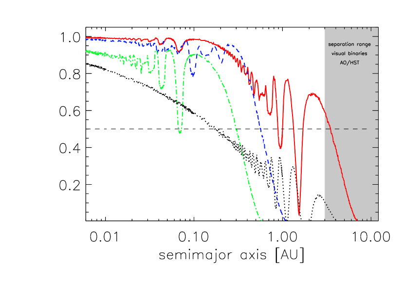
Figure 9: Comparison of detection probability of different BD/VLMS RV surveys. All curves were calculated for $q$ selected randomly from [0.2,1], random orientation, variability threshold of $p<10^{-3}$. Solid (red) line: this work (calculated for $M_{1}$=0.07 $M_{\odot}$, $\sigma_{RV}$=0.29 km s^-1, $t_{obs}$=[0,20 d,2000 d]); dotted (black) line: Basri & Reiners 2006 ($M_{1}$=0.15 $M_{\odot}$, $\sigma_{RV}$=1.3 km s^-1, $t_{obs}$=[0,1650 d]); dashed (blue) line: Guenther & Wuchterl 2003 ($M_{1}$=0.1 $M_{\odot}$, $\sigma_{RV}$=0.64 km s^-1, $t_{obs}$=[0,31 d,85 d]); dash-dotted (green) line: Kurosawa et al. 2006 ($M_{1}$=0.07 $M_{\odot}$, $\sigma_{RV}$=0.42 km s^-1, $t_{obs}$=[0,20 d]). See online version for a color figure.

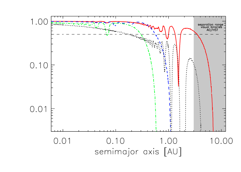
Figure 10: Same as Fig. 9 but with logarithmic y-axis to facilitate comparison with other publications. See online version for a color figure.

In the following, the detection efficiency vs. orbital separation of several current RV surveys of BD/VLMS (Guenther & Wuchterl 2003; Kurosawa et al. 2006; Basri & Reiners 2006; this work) is compared in a uniform way. For this purpose, the detection probability is calculated (i) by taking into account the average measurement uncertainties and time sequences of the individual surveys; (ii) by assuming circular orbits, random orientation, random starting orbital phase, a mass ratio chosen randomly between 0.2 and 1; and (iii) by applying a threshold for variability detection of $p<10^{-3}$. Figures 9–10 show the result. The orbital separation range that can be probed with 50% detection efficiency is $\leq$3 AU (subsample of BD/VLMS in this work), $\leq$0.6 AU (Guenther & Wuchterl 2003), $\leq$0.3 AU (Kurosawa et al. 2006), and $\leq$0.2 AU (Basri & Reiners 2006), respectively. The difference in the maximum orbital separations between the surveys by Kurosawa et al. (2006), Guenther & Wuchterl (2003), and this work can be largely attributed to differences in the covered time base. While the distribution of the detection efficiency in the survey by Basri & Reiners (2006) is non-zero for separations greater than 1  AU due to the relatively large time base, it is decreasing more rapidly compared to the other surveys. This is mainly due to the moderate RV precision of this survey, which makes it less sensitive to low-mass ratio systems. The differences of this calculated detection probability curve for the survey by Basri & Reiners (2006) compared to the one presented by the authors themselves, who find a sensitivity up to 6 AU, are the assumptions concerning inclination (random orientation instead of fixed inclination), mass ratio ($q$ selected randomly from a uniform distribution between 0.2 and 1 instead of $q$=0.5), and threshold for variability ($p<10^{-3}$, i.e. 3.3$\sigma$ instead of $p<10^{-1.347}$, i.e. 2$\sigma$). This, in addition to neglecting differences in the RV errors of different surveys, leads to a deviating picture in Fig. 4 of Basri & Reiners (2006).

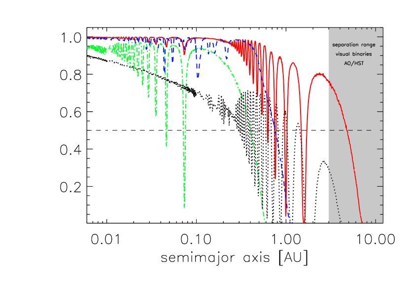
Figure 11: Comparison of detection probability of different BD/VLMS RV surveys for high-mass ratio binaries. Same as Fig. 9 but for $q$ selected randomly from [0.8,1]. See online version for a color figure.

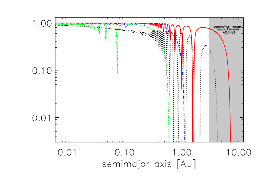
Figure 12: Same as Fig. 11 but with logarithmic y-axis to facilitate comparison with other publications. See online version for a color figure.

The BD/VLM binaries with a mass ratio close to unity cause a stronger RV signal compared to low-mass ratio systems and are, therefore, easier detected at larger separations. To quantify this, the sensitivity of the considered surveys has been calculated for binaries with mass ratios between 0.8 and 1. In this case ($q>$0.8), a 50% detection efficiency can be read off from Figs. 11 and 12 for the following separation ranges: $\leq$5 AU (subsample of BD/VLMS in this work), $\leq$2 AU (Basri & Reiners 2006), $\leq$0.8 AU (Guenther & Wuchterl 2003), and $\leq$0.4 AU (Kurosawa et al. 2006). In this mass-ratio regime, neglecting line-blending in the performed simulation is relevant (see above). At separations where the effects of line blending in the $q$ range 0.8-1.0 are significant, these detection probabilities may be significantly reduced. A comprehensive analysis of these effects is beyond the scope of this work.

For eleven objects in the survey by Basri & Reiners (2006), there are a third or more epoch observations with a temporal separation of more than one day. Such intermediate observations can positively influence the detection efficiency, as shown before. However, a simulation assuming an average observing pattern of $t_{obs}$=[0,500 d,1650 d] for this survey does not change the calculated detection probability.

5 Low-mass, long-period spectroscopic binary CHXR 74

Significant RV variability indicating the presence of a spectroscopic companion orbiting the very young low-mass star CHXR74 (M4.25-M4.5,$\sim$0.2–0.25 M_⊙, Comerón et al. 2000; Luhman 2007) has been already found by Joergens (2006a). The new RV measurements of CHXR 74 in 2005 and 2006 (Table 1) support this finding. The RV of this star is, apart from some short-term scatter, increasing almost monotonically between 2000 and 2006 (Fig. 4, bottom panel) with a recorded peak-to-peak difference of 4.8 km s^-1. The data indicate a relatively long orbital period of at least twelve years, hence, an orbital separation greater than about 3 AU. This can be used to derive a very rough estimate of the minimum companion mass $M_{2}\sin i$ of $\sim$80 $M_{\mathrm{Jup}}$. Given the relatively long orbital period for a spectroscopic system and its youth, CHXR 74 might be one of the first very young spectroscopic binaries that can be spatially resolved. A binary with a separation of more than 3 AU (20 milli arc sec at the distance of the target) might be spatially distinguished from the primary by high-resolution imaging, e.g. with NACO/VLT. If so, CHXR 74 might provide dynamical mass determinations of its components and, therefore, valuable constraints for the early evolution at the low-mass end of the stellar mass spectrum.

6 Summary and discussion

This paper presents an RV survey for close companions to very low-mass objects in the Cha I star-forming region based on UVES/VLT spectra. The survey is sensitive to companions at orbital distances of 3 AU and smaller (averaged over all objects) with a detection rate of 50% or more, as shown by a Monte-Carlo simulation. For BD/VLM binaries with a mass ratio close to unity ($q>$0.8), the survey is sensitive to even larger separations. This is a significant extension to larger orbital separations compared to previous results of this survey (Joergens 2006a), as well as compared to other RV surveys of young BD/VLMS (Kurosawa et al 2006; Prato 2007a; Maxted et al. 2008), which cover separations $\lesssim$0.3 AU, and to other surveys of field BD/VLMS (Reid et al 2002; Guenther & Wuchterl 2003; Basri & Reiners 2006), which cover separations $\lesssim$0.6 AU (comparison based on $q$ between 0.2 and 1, 3.3 $\sigma$ detection, 50% detection probability). Only the survey by Basri & Reiners (2006) has a comparable time base, however, the survey presented here is, nevertheless, superior in terms of detection efficiency mainly because of smaller RV errors. Thus, for the first time, the binary frequency of BD/VLMS is probed for the whole separation range $<$3 AU with a sensitivity to low-mass ratio systems.

Two objects were identified as spectroscopic binaries based on significant RV variability. This corresponds to an observed binary fraction of 18${}^{+20}_{-12}$ % for the whole sample of eleven BDs and (very) low-mass stars (M$\lesssim 0.25\,M_{\odot}$) and 10${}^{+18}_{-8}$ % for the subsample of ten BD/VLMS (M$\lesssim 0.1\,M_{\odot}$), respectively. The detected binaries are (i) the BD/VLMS Cha H$\alpha$ 8 (M5.75-M6.5), which has a substellar RV companion in a $\sim$1 AU orbit, as previously discovered (Joergens 2006; Joergens & Müller 2007). Cha H$\alpha$ 8 is likely the lowest mass RV companion found so far around a BD/VLMS. (ii) The low-mass star CHXR 74 (M4.25-M4.5), which has a spectroscopic companion in a relatively long-period orbit (presumably $>$12 years), as found by previous observations (Joergens 2006) and confirmed here based on new RV data. With such a relatively long period, CHXR 74 is coming into reach for being one of the first very young low-mass spectroscopic binaries that can be spatially resolved.

These spectroscopic binaries appear to have orbital periods of at least a few years, i.e. orbital separations of 1 AU or greater: (i) an RV orbit solution shows that Cha H$\alpha$ 8 has a companion in an orbit of more than four years (Joergens & Müller 2007); (ii) the companion of CHXR 74 has very likely an orbit of more than twelve years (Sect. 5). Thus, while the rate of BD/VLM binaries at $\leq$3 AU is found to be 10% (18% including CHXR 74), at separations $<$1 AU, it might be less than 10% (0/11 for the whole sample and 0/10 for the BD/VLMS subsample). There were no signs of the presence of shorter period companions around the targets. This is noteworthy because those cause stronger RV signals making them easier to detect. In fact, two out of the four BD/VLM spectroscopic binaries with determined orbital parameters (including Cha H$\alpha$ 8) have periods of only a few days (Basri & Martín 1999; Stassun et al. 2006).

There is no evidence in the cross correlation peaks of a double-lined nature of the detected binaries. This hints at a low rate of double-lined spectroscopic binaries in the sample.

In this survey, there are no large velocity amplitudes recorded (Fig. 13), as would have been expected for (nearly) equal mass binaries (e.g. a few tenths of km s^-1 for the BD binary PPl 15, Basri & Martín 1999). The detected significant RV variability occurs only on small scales: Cha H$\alpha$ 8 has an RV semi-amplitude of 1.6 km s^-1 (Joergens & Müller 2007) and a half peak-to-peak RV difference for CHXR 74 is 2.4 km s^-1. Note that an only moderate RV precision of e.g. 1.4 km s^-1, as in the survey by Basri & Reiners (2006), would have prevented the detection of these binaries. The results hint at the possibility that there exist more low-mass ratio systems among BD/VLMS, at least at $<$3 AU, than anticipated from an extrapolation from the mass-ratio distribution derived based on direct imaging surveys, which peaks at $q\sim$1 and declines rapidly for low $q$ values (e.g. Burgasser et al. 2007). On the other hand, the small RV amplitudes can also be attributed to observations at low orbital inclinations. It is, however, interesting that a preference for small RV amplitudes is also seen in RV surveys of BD/VLMS in other star-forming regions, namely in USco and $\rho$ Oph (0.2–0.5 km s^-1, Kurosawa et al. 2006, cf. also footnote 5) and in Taurus, Ophiuchus, and TW Hya (1.5–2.0 km s^-1, Prato 2007a).

Current spectroscopic surveys of very low-mass objects differ widely in the studied parameter ranges, as orbital separations, (primary and) companion masses, and environments/ages. Within the (sometimes large) statistical errors, the determined binary frequencies are largely consistent and range between $<$7.5% and 24%: 10${}^{+18}_{-8}$ % for ten BD/VLMS in Cha I at $\leq$3 AU (this work), 24${}^{+16}_{-13}$ % for 17 BD/VLMS in USco and $\rho$ Oph at $\leq$0.3 AU (Kurosawa et al. 2006), 17% for 18 BD/VLMS in Taurus, Ophiuchus, and TW Hya at $\lesssim$0.3 AU (Prato 2007a), $<$7.5% for 51 BD/VLM member candidates of $\sigma$ and $\lambda$ Orionis at $\leq$0.3 AU (Maxted et al. 2008), 12${}^{+11}_{-7}$ % for 25 field and cluster dwarfs at $\leq$0.6 AU (Guenther & Wuchterl 2003), and 11${}^{+7}_{-4}$ % for 53 (very) low-mass field stars and BDs at $\leq$0.2 AU ($\leq$1-2 AU for $q>$0.8) (Basri & Reiners 2006).

By combining my work in Cha I with other RV surveys of young regions, an overall BD/VLM binary fraction at an age of a few million years can be derived. With the exception of Cha I, all RV surveys of young BD/VLMS probe only a narrow separation range ($\lesssim$0.3 AU). No companions are found orbiting BD/VLMS in Cha I at these separations. Thus, the overall observed binary fraction at separations $\leq$0.3 AU of very young BD/VLMS in Cha I (0/10), USco and $\rho$ Oph (4/17, Kurosawa et al. 2006), Taurus, Ophiuchus, and TW Hya (3/18, Prato 2007a), and $\sigma$ and $\lambda$ Orionis (0/52, Maxted et al. 2008) is 7${}^{+5}_{-3}$% (7/97).

Comparing the binary frequency of BD/VLMS in ChaI for separations $\leq$3 AU (10${}^{+18}_{-8}$ %) with what is determined based on direct (adaptive optics and HST) imaging surveys at larger separations ($>$20 AU) in the same star-forming region (9${}^{+17}_{-7}$%, Neuhäuser et al 2002; Neuhäuser, Guenther & Brandner 2003; 11${}^{+9}_{-6}$%, Ahmic et al 2007), one finds consistent values.

7 Conclusions

For the first time, the binary frequency of BD/VLMS is probed in the orbital separation range 1–3 AU. The separation distribution of BD/VLM binaries detected by direct imaging surveys (e.g. Burgasser et al. 2007) has a peak around 3–10 AU, which is close to the incompleteness limit of these surveys ($<$2–3 AU for the field and $<$10-15 AU for star-forming regions, respectively). It seemed, therefore, possible that the largest fraction of BD/VLM binaries has separations in the range of about 1–3 AU and still remained undetected. The BD/VLM binary frequency of 10${}^{+18}_{-8}$ % determined here at separations of 3 AU and smaller shows that this is not the case because the rate of spectroscopic binaries at $<$3 AU does not significantly exceed the rate of resolved binaries at larger separations (10–30%, e.g. Burgasser et al. 2007). Thus, the separation range $<$3 AU missed by direct imaging surveys is not adding a significant fraction to the BD/VLM binary frequency, and the overall binary frequency of BD/VLMS is in the range 10-30%. The finding of no signs (0/10, i.e. $\leq$10%) for companions at $<$1 AU is consistent with a decline in the separation distribution of BD/VLM binaries towards smaller separations starting between 1 and 3 AU. Furthermore, the previous finding that the observed mass-dependent decrease in the stellar binary frequency (e.g. Delfosse et al. 2004; Shatsky & Tokovinin 2002; Kouwenhoven et al. 2005) continuously extends into the BD regime (e.g. Burgasser et al. 2007) is confirmed here for separations $<$3 AU. This is consistent with a continuous formation mechanism from low-mass stars to BDs.

These results are based on a relatively small sample. By combining this work in Cha I with surveys of other young regions, which are restricted to separations $\leq$0.3 AU, an overall observed binary fraction of very young BD/VLMS can be determined with better statistics but with a more limited separation range. In this way, a binary frequency of 7${}^{+5}_{-3}$% (7/97) is found at $\leq$0.3 AU. In the near future, the sample of the survey in Cha I will be substantially enlarged, allowing the re-investigation of the binary frequency at $<$3 AU of BD/VLMS in Cha I with significantly improved statistics for a uniformly obtained data set. Current and future observational efforts are, in addition, directed towards determination of orbital parameters of the detected binary systems, including RV follow-up and high-resolution imaging/astrometry.

Table 1: New RV measurements for BDs and VLMSs in Cha I.

Object	Date	HJD	RV	$\sigma_{RV}$
			[km s-1]	[km s-1]
Cha H$\alpha$ 1	2006 Jan 16	2453751.74004	16.206	0.39 *
Cha H$\alpha$ 2	2006 Jan 16	2453751.79554	16.319	0.25 *
Cha H$\alpha$ 3	2006 Jan 15	2453750.81659	16.339	0.70 *
Cha H$\alpha$ 5	2006 Jan 15	2453750.84774	15.697	0.03 *
Cha H$\alpha$ 6	2006 Jan 16	2453751.82994	16.630	0.07 *
Cha H$\alpha$ 7	2006 Jan 15	wrong pointing
Cha H$\alpha$ 12	2006 Jan 17	2453752.70145	15.831	0.05 *
B 34	2005 Nov 25	2453699.83976	15.687	0.10 *
CHXR 74	2005 Mar 21	2453450.58923	18.185	0.06 *
	2006 Apr 10	2453835.63456	17.982	0.10
	2006 Jun 15	2453901.52267	19.063	0.10

Table 2: Characteristics of observations and $\chi^{2}$ probabilities.

Object	$\Delta$ RV	$\overline{\mathrm{RV}}_{weighted}$	no. obs	Min. $\Delta$t	Max. $\Delta$t	p
	[km s-1]	[km s-1]		[days]	[days]
Cha H$\alpha$ 1	0.24	16.27 $\pm$ 0.52	3	20	2113	8.3 $\times 10^{-1}$
Cha H$\alpha$ 2	0.15	16.25 $\pm$ 0.49	3	20	2113	8.7 $\times 10^{-1}$
Cha H$\alpha$ 3	0.99	14.86 $\pm$ 0.89	3	19	2111	5.6 $\times 10^{-2}$
Cha H$\alpha$ 4	0.21	14.85 $\pm$ 0.43	11	1	701	1.0
Cha H$\alpha$ 5	0.13	15.59 $\pm$ 0.48	3	19	2111	8.7 $\times 10^{-1}$
Cha H$\alpha$ 6	0.28	16.52 $\pm$ 0.56	3	19	2112	6.3 $\times 10^{-1}$
Cha H$\alpha$ 7	0.58	17.09 $\pm$ 0.98	2	19	19	1.5 $\times 10^{-1}$
Cha H$\alpha$ 8	1.38	16.62 $\pm$ 0.67	11	3	2542	0.0	vari.
Cha H$\alpha$ 12	0.96	15.29 $\pm$ 0.93	3	20	2113	5.6 $\times 10^{-3}$
B 34	0.07	15.74 $\pm$ 0.42	6	6	2083	1.0
CHXR 74	2.39	16.71 $\pm$ 0.81	13	1	2285	0.0	vari.

Figure 1: RV measurements of Cha H$\alpha$ 1, Cha H$\alpha$ 2, Cha H$\alpha$ 3 (top to bottom).

Figure 2: RV measurements of Cha H$\alpha$ 4, Cha H$\alpha$ 5, Cha H$\alpha$ 6 (top to bottom).

Figure 3: RV measurements of Cha H$\alpha$ 7 and Cha H$\alpha$ 12 (top to bottom).

Figure 4: RV measurements of B 34 and CHXR 74 (top to bottom).

Figure 5: Histogram of the $\chi^{2}$ probability $p$ for fitting the observed (relative) RV values of the BD/(V)LMS in Cha I studied here with a constant function. Objects with $p<10^{-5}$ are shown in the right-most bin, Cha H$\alpha$ 8 and CHXR74. Based on the threshold $p<10^{-3}$, they are classified as binaries. Overplotted is the expected distribution for nonvariable objects given the estimated uncertainties. It shows that the error estimates are reliable.

Figure 6: Detection probability as function of semi-major axis. Based on a Monte Carlo simulation of RV measurements for randomly selected binaries using the measurement errors and time separations of the real observations. From top to bottom: Cha H$\alpha$ 7; average of Cha H$\alpha$ 1 and Cha H$\alpha$ 3; average of Cha H$\alpha$ 2, Cha H$\alpha$ 4, Cha H$\alpha$ 5, Cha H$\alpha$ 6, Cha H$\alpha$ 8, and Cha H$\alpha$ 12; B 34; and CHXR 74. As indicated, some curves are the average detection probability for two or more objects because observations have similar quality for those.

Figure 7: Dependence of detection probability on assumption about inclination. Both curves are calculated for $M_{1}$=0.07 $M_{\odot}$, $\sigma_{RV}$=0.29 km s^-1, $t_{obs}$=[0,20 d,2000 d], and $q$ selected randomly from [0.2,1]. Assuming a fixed mean inclination value (dotted line), as in Basri & Reiners (2006), slightly overestimates the detection efficiency compared to the realistic case of random orientation (solid line). For the fixed inclination case, the mean value of the inclination distribution of 57.3^∘ is used.

Figure 8: Dependence of detection probability on number of observations. Both curves are calculated for $M_{1}$=0.07 $M_{\odot}$, $\sigma_{RV}$=0.29 km s^-1, a maximum time span of 2000 d, $q$ selected randomly from [0.2,1], and random orientation. An observing schedule based on three observations with $t_{obs}$=[0,20 d,2000 d] (solid line) provides a superior detection efficiency compared to the case of only two observations separated by 2000 d ($t_{obs}$=[0,2000 d], dotted line). Thus, third-epoch observations between the observations with the largest time difference can have a significant effect on the probability distribution.

Figure 13: RV differences vs. object mass. Plotted are half peak-to-peak differences in the observed RVs. Each data point is labeled with the corresponding object name, the numbers denote the Cha H$\alpha$ objects. The RV variable objects (CHXR 74, Cha H$\alpha$ 8) have $\Delta$RV $\gtrsim$ 1.4 km s^-1, while the majority of RV constant objects have $\Delta$RV $\leq$0.3–0.6 km s^-1, with the exception of Cha H$\alpha$ 3 and Cha H$\alpha$ 12, which have $\Delta$RV $\sim$1 km s^-1.

Figure 14: RV differences for BD/VLMS in USco and $\rho$ Oph based on data from Kurosawa et al. (2006). $\Delta$RV as in Fig. 13. Objects classified as RV variables by these authors are denoted with their names. The two data points with the largest RV difference correspond to GY310 and USco101, which are classified as RV constant.

- (1) Ahmic, M., Jayawardhana, R., Brandeker, A., Scholz, A., van Kerkwijk, M. H. 2007, ApJ, 671, 2074
- (2) Basri, G., & Martín, E. L. 1999, ApJ 118, 2460
- (3) Basri, G., & Reiners A. 2006, ApJ 132, 663
- (4) Bate, M. R., Bonnell, I. A., & Bromm, V. 2002, MNRAS 332, L65
- (5) Bate, M. R., Bonnell, I. A., & Bromm, V. 2003 MNRAS 339, 577
- (6) Boss, A., 2001, ApJ 551, L167
- (7) Bouy, H., Brandner, W., Martín, E. L., Delfosse, X., Allard, F., & Basri, G. 2003, AJ 126, 1526
- (8) Burgasser, A. J., Kirkpatrick, J. D., Reid, I. N., Brown M. E., Miskey C. L. et al. 2003, AJ 586, 512
- (9) Burgasser, A. J., Reid, I. N., Siegler, N., Close, L., Allen, P., Lowrance, P. & Gizis J., 2007, in Protostars and Planets V, ed. by B. Reipurth, D. Jewitt & K. Keil (Tucson, University of Arizona Press), 427
- (10) Close, L. M., Siegler, N., Freed, M. & Biller, B. 2003, ApJ 587, 407
- (11) Comerón, F., Rieke, G. H., & Neuhäuser, R. 1999, A&A, 343, 477
- (12) Comerón, F., Neuhäuser, R., & Kaas, A. A. 2000, A&A, 359, 269
- (13) Delfosse, X., Beuzit, J.-L., Marchal, L., Bonfils, X. C., Perrier, C. et al. 2004, in ASP Conf. Ser. 318, ed. by R. W. Hidlitch, H. Hensberge & K. Pavlovski, San Francisco, 166
- (14) Gizis, J. E., Reid, I. N., Knapp, G. R., Liebert, J., Kirkpatrick J. D., et al. 2003, AJ 125, 3302
- (15) Goodwin, S. P. & Whitworth, A. 2007, A&A, 466, 943
- (16) Guenther, E. W., & Wuchterl, G. 2003, A&A 401, 677
- (17) Joergens, V., & Guenther, E. 2001, A&A, 379, L9
- (18) Joergens, V., Fernández, M., Carpenter, J. M., & Neuhäuser, R. 2003, ApJ 594, 971
- (19) Joergens, V. 2006a, A&A 446, 1165
- (20) Joergens, V. 2006b, A&A 448, 655
- (21) Joergens, V., & Müller, A. 2007, ApJ 666, L113
- (22) Kenyon, M. J., Jeffries, R. D., Naylor, T., Oliveira, J. M. & Maxted, P. F. L. 2005, MNRAS, 356, 89
- (23) Kouwenhoven, M. B. N., Brown, A. G. A., Zinnecker, H., Kaper, L., Portegies Zwart, S. F. 2005, A&A, 430, 137
- (24) Kroupa, P., & Bouvier, J. 2003b, MNRAS 346, 369
- (25) Kurosawa, R., Harries, T. J., & Littlefair, S. P. 2006, MNRAS 372, 1879
- (26) Luhman, K. L. 2004, ApJ 614, 398
- (27) Luhman, K. L. 2007, ApJS 173, 104
- (28) Luhman, K., Joergens, V., Lada, C., Muzerolle, J., Pascucci, I. & White, R., 2007, in Protostars and Planets V, ed. by B. Reipurth, D. Jewitt, K. Keil, (Tucson, University of Arizona Press), 443
- (29) Maxted, P. F. L., & Jeffries, R. D. 2005 MNRAS 362, L45
- (30) Maxted, P. F. L., Jeffries, R. D., Oliveira J. M., Naylor T. & Jackson R. J. 2008, MNRAS 385, 2210
- (31) Mizuno, A., Hayakawa, T., Tachihara, K. et al. 1999, PASJ 51, 859
- (32) Neuhäuser, R., Brandner, W., Alves, J., Joergens, V., & Comerón, F. 2002, A&A, 384, 999
- (33) Neuhäuser, R., Brandner, W., & Guenther, E. 2003, IAUS 211, 309, ed. by E. Martín
- (34) Padoan, P. & Nordlund, A. 2004, ApJ, 617, 559
- (35) Pinfield, D. J., Dobbie, P. D., Jameson, R. F., Steele, I. A., Jones, H. R. A., et al. 2003, MNRAS 342, 1241
- (36) Prato, L. 2007a American Astronomical Society Meeting Abstracts, 211, 134.22
- (37) Prato, L. 2007b, ApJ 657, 338
- (38) Reid, I. N., Gizis, J. E., Kirkpatrick, J. D. & Koerner, D. W. 2001, AJ 121, 489
- (39) Reid, I. N., Kirkpatrick, J. D., Liebert, J. Gizis, J. E., Dahn, C. C. & Monet, D. G. 2002, AJ 124, 519
- (40) Reipurth, B. & Clarke, C. 2001, AJ, 122, 432
- (41) Shatsky, N, & Tokovini, A. 2002, A&A 382, 92
- (42) Simon, M., Bender, C. & Prato, L. 2006, ApJ 644, 1183
- (43) Stamatellos, D., Hubber, D. A., & Whitworth A. P. 2007, MNRAS 382, L30
- (44) Stassun, K. G., Mathieu, R. D. & Valenti, J. A. 2006, Nature 440, 311
- (45) Sterzik, M. F., & Durisen, R. H. 2003, A&A, 400, 1031
- (46) Umbreit, S., Burkert, A., Henning, T., Mikkola, S., & Spurzem, R. 2005, ApJ, 623, 940
- (47) Whitworth, A. P., & Zinnecker, H. 2004, A&A, 427, 299
- (48) Zapatero Osorio, M. R., Lane, B. F., Pavlenko, Ya., Martín E. L., Britton, M. & Kulkarni, S. R. 2004, ApJ 615, 958