Towards M2-brane Theories for Generic Toric Singularities

Abstract:

We construct several examples of $(2+1)$ dimensional ${\cal N}=2$ supersymmetric Chern-Simons theories, whose moduli space is given by non-compact toric Calabi-Yau four-folds, which are not derivable from any (3+1) dimensional CFT. One such example is the gauge theory associated with the cone over $Q^{111}$. For several examples, we explicitly confirm the matter content, superpotential interactions and RG flows suggested by crystal models. Our results provide additional support to the idea that crystal models are relevant for describing the structure of these CFTs.

1 Introduction

Until recently, the AdS₄/CFT₃ correspondence was underdeveloped compared with its cousin AdS₅/CFT₄ [1, 2, 3]. One of the main reasons for that was our lack of understanding of CFT₃ underlying M2 brane theories probing a Calabi-Yau four-fold. M2-brane theories remained elusive compared with the theories of D3-branes, which can be studied by the usual open string analysis. Even the simplest CFT₃ theory corresponding to M2-branes probing $\mathbb{C}^{4}$ seemed to pose great difficulty. Since it has ${\cal N}=8$ supersymmetry and apparently it was difficult to go beyond ${\cal N}=3$ supersymmetry in a (2+1)d field theory, the M2 theory was regarded as some unknown field theory yet to be constructed. Recently, the status quo has changed drastically. One of the key observations was made by Schwarz [4]. He suggested that by introducing Chern-Simons terms and turning off the gauge kinetic terms in a suitable limit, one can construct (2+1)d field theories with more than ${\cal N}=3$ supersymmetry. One avatar of such idea, in retrospect, was constructed by Bagger and Lambert [5, 6, 7] and independently by Gustavsson [8, 9]. At first sight, a key role was played by 3-algebras, which do not have a usual field theory structure. Subsequently, it was shown that the theory can be recast as an ordinary field theory [10]. Since then, we have rapidly piled up various higher supersymmetric theories of Chern-Simons theories with ${\cal N}=6$, $5$, $4$ and $3$ [12, 13, 14, 15, 16, 17, 18, 19, 20], increasing the number of understandable AdS₄/CFT₃ pairs. In particular, the conjectured CFT₃ dual of coincident M2-branes probing $\mathbb{C}^{4}$ is the ${\cal N}=6$ CS theory worked out by Aharony, Bergman, Jafferis and Maldacena (ABJM). Various checks of this proposal have been performed, such as computing the moduli space, superconformal index [21] and higher order interactions due to instantons [22]. ${\cal N}=4$ theories for M2-branes on $(\mathbb{C}^{2}/\mathbb{Z}_{n})^{2}$ and orientifolds thereof were constructed in [14].

In the case of D3-branes, the AdS₅/CFT₄ correspondence has a very rich structure of theories with ${\cal N}=1$ supersymmetry (i.e. four supercharges) [24, 25, 26, 27]. The most comprehensive class of dual pairs has been achieved for D3-branes probing non-compact toric Calabi-Yau 3-folds. Given this situation, one might wonder if similar structures have yet to be discovered in AdS₄/CFT₃ with ${\cal N}=2$ supersymmetry (namely four supercharges). Several authors have already initiated such study [28, 29, 30, 31]. So far the field theory constructions have been restricted to those derived from (3+1)d theories, i.e. theories with the same quiver diagrams and superpotentials as those of (3+1)d. This represents considerable progress, but this set of theories is far from generic. One should go beyond this approach to attack general ${\cal N}=2$ AdS₄/CFT₃. Here we initiate such study. In the current paper, we construct several examples of the theories which cannot come from the (3+1)d quiver theories. One famous example is the theory of M2-branes probing the cone over $Q^{111}$, which is expected to have a sextic superpotential. This theory is the (2+1)d analogue of the theory of D3-branes probing the conifold worked out by Klebanov and Witten [32]. Using the recently developed formalism of [29] and partly guided by crystal models [33, 34, 35], we explicitly construct a (2+1)d theory whose moduli space is indeed $C(Q^{111})$, where $C(M)$ denotes the cone over the manifold $M$. In addition, we work out several other theories that cannot have a (3+1)d origin. Obviously, our constructions just touch the tip of an iceberg and an extensive investigation of all related issues is beyond the scope of the current paper. One feature worth mentioning, though, is that there can be more than one theory with the same moduli space. This is reminiscent of Seiberg duality or toric duality [36, 37] in (3+1)d. Apparently, there are far more possibilities in (2+1)d than in (3+1)d.

The paper is organized as follows. In section 2, we briefly summarize some aspects of ${\cal N}=2$ Chern-Simons theories with matter and crystal models needed for later sections. In section 3, we mention some features of (2+1)d theories derivable from (3+1)d and try to characterize them. In section 4, we construct the theory whose moduli space is $C(Q^{111})$. In section 5, we construct the theory for $C(dP_{3})\times\mathbb{C}$ and show that, upon addition of masses for adjoint fields, it is connected to that of $C(Q^{111})$ by an RG-flow. This RG flow is suggested by crystal models. In section 6.1, we construct another pair of models related by a similar RG-flow, the theories for $D_{3}$ and $\mathbb{C}^{3}/(\mathbb{Z}_{2}\times\mathbb{Z}_{2})\times\mathbb{C}$. Interestingly, the theories in section 6.1 are related to those in sections 4 and 5 by a simple flip in the charges of some matter fields. In section 6.2, we propose the CS theories for $\mathbb{C}^{3}/(\mathbb{Z}_{n}\times\mathbb{Z}_{n})\times\mathbb{C}$. This proposal is explicitly checked for $n=3$ in appendix A. Section 7 discusses partial resolution and how it connects the theories we have studied. We conclude in section 8. In appendix B, we present some thoughts about parity invariance in these models.

2 Preliminaries

2.1 Moduli spaces of (2+1)d CS theories

The moduli space of the theories of our interest can be computed following [29]. We now summarize the procedure. A (2+1)d ${\cal N}=2$ Chern-Simons(CS) theory with bifundamental and adjoint matter is given, in ${\cal N}=2$ superspace notation, by the following Lagrangian

$${\rm Tr}\left(-\int d^{4}\theta\sum_{X_{ab}}X_{ab}^{\dagger}e^{-V_{a}}X_{ab}e^{V_{b}}-i\sum_{a}k_{a}\int_{0}^{1}dtV_{a}\bar{D}^{\alpha}(e^{tV_{a}}D_{\alpha}e^{-tV_{a}})+\int d^{2}\theta W(X_{ab})+{\rm c.c.}\right)~{},$$ (2.1)

where $V_{a}$ are vector supermultiplets and $X_{ab}$ denote chiral supermultiplets transforming in the fundamental representation of gauge group $a$ and the anti-fundamental representation of gauge group $b$. For $a=b$, this corresponds to adjoint matter for gauge group $a$. We take $\sum k_{a}=0$. This is a necessary condition for the moduli space to be four complex dimensional. Recall that in 2+1 dimensions a vector superfield has the expansion

$$V=-2i\theta\bar{\theta}\sigma+2\theta\gamma^{\mu}\bar{\theta}A_{\mu}+\cdot\cdot\cdot+\theta^{2}\bar{\theta}^{2}D~{},$$ (2.2)

where we omitted the fermionic part. Compared to 3+1 dimensions, there is a new scalar field $\sigma$. We can write all terms contributing to the scalar potential in the Lagrangian

$${\rm Tr}\left(-4\sum_{a}k_{a}\sigma_{a}D_{a}+\sum_{a}D_{a}\mu_{a}(X)-\sum_{X_{ab}}(\sigma_{a}X_{ab}-X_{ab}\sigma_{b})(\sigma_{a}X_{ab}-X_{ab}\sigma_{b})^{\dagger}-\sum_{X_{ab}}|\partial_{X_{ab}}W|^{2}\right)~{}.$$ (2.3)

$\mu_{a}(X)$ is the moment map for the $a$-th gauge group

$$\mu_{a}(X)=\sum_{b}X_{ab}X_{ab}^{\dagger}-\sum_{c}X_{ca}^{\dagger}X_{ca}+[X_{aa},X_{aa}^{\dagger}]~{},$$ (2.4)

and gives the D-term. Here we use the same terminology of (3+1)d.

By integrating out the auxiliary fields $D_{a}$, we see that the bosonic potential is a sum of squares. The vacua can be found by looking for vanishing of the scalar potential. This gives rise to a set of matrix equations

$$\partial_{X_{ab}}W = 0$$

$$\mu_{a}(X) = 4k_{a}\sigma_{a}$$

$$\sigma_{a}X_{ab}-X_{ab}\sigma_{b} = 0$$ (2.5)

The solutions to these equations automatically satisfy $D_{a}=0$ and correspond to supersymmetric vacua. F-term constraints are exactly as in the (3+1)d case, while D-term constraints are modified. The solution to only the F-terms is a useful object called the master space [38], which is also a toric variety.

Let us consider the abelian case. The supersymmetric conditions set all $\sigma_{a}$ equal to a given value $\sigma$. The remaining equations

$$\mu_{a}(X)=4k_{a}\sigma$$ (2.6)

look like standard D-term equations with a set of effective FI terms $\zeta_{a}=4k_{a}\sigma$. Since $\sum_{a}k_{a}=0$, one of these equations is redundant. Call $G$ the number of gauge groups. We are left with $G-1$ equations. By taking integer linear combinations of the equations, we can set $G-2$ equations to the form

$$\tilde{\mu}_{i}(X)=0\,,\qquad\qquad i=1,...G-2$$ (2.7)

where the index $i$ identifies $G-2$ linear combinations of the gauge group, orthogonal to the direction determined by the FI parameters $\zeta_{a}$. These combinations are easily identified as the kernel of the following matrix [43]

$$C=\left(\begin{array}[]{ccccc}\ 1&\ 1&\ \ldots&\ 1&\ 1\\ k_{1}&k_{2}&\ldots&k_{G-1}&k_{G}\end{array}\right)~{}.$$ (2.8)

We see that we are imposing the vanishing of the D-terms for $G-2$ $U(1)$ gauge groups. As usual, combining D-term constraints with U(1) gauge transformations is equivalent to modding out by the complexified gauge group. The equation for the remaining $U(1)$ gauge field looks like a D-term condition with a FI term. However, it does not add further constraints: it simply determines the value of the auxiliary field $\sigma$. Analogously we do not need to mod out by the remaining $U(1)$ gauge group. As explained in detail in [11, 12], the $U(1)$ is coupled to the overall $U(1)$ gauge field by the Chern-Simons coupling and leaves a discrete symmetry $\mathbb{Z}_{k}$, where $k=\gcd(\{k_{a}\})$. Note that since we are obtaining the 4-complex dimensional moduli space by imposing $G-2$ D-terms, the master space is $G+2$ dimensional.

The moduli space is non-compact CY₄-fold and is interpreted as the transverse space to one M2-brane in M-theory probing such geometry. In the non-abelian case, the moduli space is the symmetric product of $N$ copies of the abelian moduli space [29].

The computation of the moduli space closely resembles the (3+1)d case, with a simple modification concerning D-terms. In practice, we will use the machinery of toric geometry. We refer the reader to [36], to which notation we adhere, for a comprehensive review of its application to this problem.

We close this section with a comment on two classes of models: those in which all $k_{i}\neq 0$ and those in which some $k_{i}=0$. For the first class, all vector multiplets become massive and hence it is easier to think about their IR limit. On the other hand, we can also argue that there is no objection to considering models in the second class. When computing the moduli space, we quotient by the $U(1)$ gauge group(s) with $k_{i}=0$. Hence, we only consider variables that are invariant under these gauge group(s). We can think about the corresponding gauge fields as auxiliary fields (Lagrange multipliers). For all the quivers in this paper, we find CS levels in both classes that reproduce the desired geometries. Since both of them seem to work at the level accessible at the moment, we list both possibilities.

2.2 Minimal review of crystal models

We now give a brief review of the M-theory crystal models [33, 34, 35]. Crystal models relate a toric CY₄ to a three-dimensional periodic graph (crystal). This crystal is conjectured to encode information about the CFT₃ on M2-branes probing the corresponding CY₄.

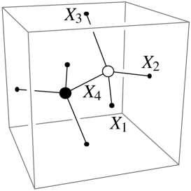
Figure 1: Crystal of $\mathbb{C}^{4}$ adopted from [34].

The toric diagram forms a convex polyhedron in $\mathbb{Z}^{3}\subset\mathbb{Z}^{4}$. The reduction from $\mathbb{Z}^{4}$ to $\mathbb{Z}^{3}$ is a consequence of the CY condition. The crystal model follows from a T-duality of M-theory. We take the T-duality transformation along a $T^{3}\subset T^{4}$ aligned with the projection $\mathbb{Z}^{4}\rightarrow\mathbb{Z}^{3}$. This corresponds to the $x^{6,7,8}$ directions in Table 1. By T-duality, we mean the element $t$ in the $SL(2,\mathbb{Z})\times SL(3,\mathbb{Z})$ duality group which acts as $t:\tau\equiv C_{(3)}+i\sqrt{g_{T^{3}}}\rightarrow-1/\tau$. The stack of $N$ M2-branes turns into a stack of $N$ M5-branes wrapping the dual $T^{3}$. We call them the $T$-branes. The degenerating circle fibers turn into another M5-brane extended along the (2+1)d world-volume and a non-trivial 3-manifold $S$ in ${\rm I\kern-1.79993ptR}^{3}\times T^{3}$. We call it the $S$-brane. Preservation of supersymmetry requires that the $S$-brane wrap a special Lagrangian submanifold of ${\rm I\kern-1.79993ptR}^{3}\times T^{3}=(\mathbb{C}^{*})^{3}$, and that it is locally a plane in ${\rm I\kern-1.79993ptR}^{3}$ and a 1-cycle in $T^{3}$. The result is summarized in Table 1.

$$\begin{array}[]{l|ccc|cccccc|cc}\hline\cr&0&1&2&3&4&5&6&7&8&9&11\\ \hline\cr\mbox{M5}&\circ&\circ&\circ&&&&\circ&\circ&\circ\\ \mbox{M5}&\circ&\circ&\circ&\lx@intercol\hfil\Sigma\hfil\lx@intercol\vrule\lx@intercol&&\\ \hline\cr\end{array}$$

Table 1: The brane configuration for M2 theories probing a toric CY₄.

The crystal graph is the intersection locus between the $T$-branes and the $S$-brane projected onto the $T^{3}$. Figure 1, shows the crystal for $\mathbb{C}^{4}$. We have 4 bonds and 2 vertices. In crystal models each bond represents a ${\cal N}=2$ chiral field. As in dimer models, it is easy to read off the superpotential from crystal models. Every vertex in the crystal contributes a term in the superpotential, given by the product of all the fields meeting at a vertex, with a positive sign for white vertices and a negative sign for black ones. In Figure 1, we see that we have four chiral fields and two superpotential terms. It is not clear how to read off the gauge group from the crystal model compatible with the CS theories proposed so far, though there has been partial success [35]. The proposal in [43] seems to be promising for solving this problem. The ABJM model has four bifundamental chiral multiplets and the superpotential is identified with that of the conifold (3+1)d theory [12]. This is in perfect agreement with the structure suggested by Figure 1. We will see later that there is another possibility for assigning gauge groups to the above crystal.

An important concept is that of a perfect matching. It is a collection of bonds such that every node in the crystal belongs to exactly one bond. In (3+1)d, it has been shown that there is a one to one correspondence between perfect matchings in the dimer model and GLSM fields describing the moduli space [44]. The same is true for the case of crystals, since it is straightforward to show that perfect matchings are good variables for solving F-term equations. While all the calculations in the coming sections can be performed without any reference to perfect matchings, it is sometimes practical to use this correspondence.

In addition, crystal models seem to be very useful in clarifying such issues as RG-flows, partial resolution and toric-duality in the (2+1)d setting. One can also use crystal models to work out the meson spectrum of the corresponding CFT₃, which is an important check of AdS₄/CFT₃ correspondence. In what follows, we use the information on the superpotential and RG-flow obtained from crystal models to guide the construction of some (2+1)d theories.

3 (2+1)d theories with and without (3+1)d parents

Recently, various authors discussed the possibility of generating (2+1)d CS theories with toric CY₄ moduli spaces by taking theories with the same quiver diagrams and superpotentials of theories in (3+1)d [28, 29, 30, 31]. We will refer to these models as theories with (3+1)d parents. While this represents an interesting progress that allows the construction of an infinite number of new models, it is not the generic situation and gives a reduced subset of theories for M2-branes over toric CY₄ manifolds. It is possible to give a very intuitive characterization of all these theories. They are theories whose 3d toric diagrams can be projected down to the 2d toric diagrams of the parent theories [43]. All known theories with (3+1)d parents satisfy this property. When projected, an important role is played by the multiplicity of GLSM fields [36, 37, 39], namely the multiplicity of every node in the toric diagram has to match the one computed from a (3+1)d theory. It turns out that all (2+1)d CS theories with toric moduli spaces that have been studied in the literature, even before the aforementioned references, fall into this subclass of models with (3+1)d parents. Figure 2 shows a sample collection of those models and their projections. Interestingly, some models like $(b)$ admit more than one projection. If projected down, it gives the toric diagram of $C(F_{0})$, a chiral $\mathbb{Z}_{2}$ orbifold of the conifold. If projected sideways, it gives the toric diagram of a non-chiral $\mathbb{Z}_{2}$ orbifold of the conifold (also denoted the cone over $L^{222}$). In these cases, the coincidence of moduli spaces can be verified by direct computation. Interestingly, both theories have the same moduli space but, naively, different amounts of supersymmetry. While the first one seems to have ${\cal N}=2$, the second one has ${\cal N}=4$. It is natural to expect that SUSY is enhanced in the first model. We will explore these issues in future work.

\psfrag{C4 to conifold}[cc][.8]{a) $\mathbb{C}^{4}\to C(T^{11})$}\psfrag{(C2/Z2)2 to F0}[cc][.8]{b) $(\mathbb{C}^{2}/\mathbb{Z}_{2})^{2}\to C(F_{0})$, $C(L^{222})$}\psfrag{conifold x C to C2/Z2 x C}[cc][.8]{c) $C(T^{11})\times\mathbb{C}\to\mathbb{C}^{2}/\mathbb{Z}_{2}\times\mathbb{C}$}\psfrag{M32 to dP0}[cc][.8]{d) $C(M^{32})\to C(dP_{0})$}\includegraphics[width=369.88582pt]{toric_projections.eps}

Figure 2: 3d toric diagrams and their projection to the 2d toric diagrams of the parents. (a) is the well known ABJM theory. It projects down to the conifold, from which it borrows the quiver and superpotential. How the 2d toric diagram is ‘inflated’ into a 3d one depends on the choice of CS levels. The number appearing in the toric diagram denotes the multiplicity of the particular node. The multiplicity is one unless otherwise stated. (b) admits two projections (indicated in green and red) to toric diagrams coming from (3+1)d theories.

Conversely, the projection prescription gives us a way to identify ‘pure’ (2+1)d theories, namely those without (3+1)d parents. They are simply those whose toric diagrams cannot be projected into 2d ones. A prototypical example is the cone over $Q^{111}$. It is interesting to work out some pure (2+1)d theories in order to understand their general structure and why they do not allow (3+1)d parents. This is the subject of our next section.

4 Gauge theory for $C(Q^{111})$

We now construct the gauge theory for $C(Q^{111})$. Very much like the conifold in (3+1)d, $C(Q^{111})$ is a great starting point due to its large symmetry. We will extract from crystals as much information as possible, assuming their correctness. We will later see that they are indeed right, by performing various checks, including the computation of the moduli space. From crystal model constructions [34, 35], we know that $C(Q^{111})$ has:

• 6 chiral fields.

• 2 non-vanishing superpotential terms of order 6.

Since the theory has two terms in the superpotential, there are no restrictions on the abelian moduli space coming from $F$-terms. In other words, the superpotential vanishes in the abelian case and the master space is $\mathbb{C}^{6}$. Then, we must have 2 constraints from D-terms, i.e., $G-2=2$ (with $G$ the number of gauge groups), thus we also know the theory has 4 gauge groups. Finally, it is given by an $SU(2)^{3}/U(1)^{2}$ coset, which has $SU(2)^{3}\times U(1)_{R}$ global symmetry. This structure appears clearly in our construction. The presence of 6 chiral fields is not surprising, since this is the minimal matter content we can think of in a theory with $SU(2)^{3}$ symmetry. One can try to construct a theory that meets all the requirements above. The constraints are so strong that the answer is basically unique. Figure 3 shows the proposed quiver diagram. We will then subject this theory to various tests.

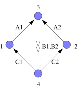
Figure 3: Quiver diagram for $Q^{111}$.

The superpotential is given by

$$W=C_{1}A_{1}B_{1}C_{2}A_{2}B_{2}-C_{1}A_{1}B_{2}C_{2}A_{2}B_{1}~{}.$$ (4.9)

In this and coming expressions, color indices are contracted between adjacent fields and a trace is implicit. The theory has an explicit $SU(2)$ global symmetry under which $B_{1}$ and $B_{2}$ form a doublet, as well as a $U(1)_{R}$ symmetry. A useful intermediate step in the computation of the mesonic moduli space is the master space. To find it, we look for solutions of F-term equations without imposing gauge invariance. As in any (toric) theory with two superpotential terms, we obtain $Q_{F}=0$ and the GLSM fields (equivalently perfect matchings) are identified with the chiral fields. Let us call $(p_{1},p_{2},p_{3},p_{4},p_{5},p_{6})=(A_{1},A_{2},B_{1},B_{2},C_{1},C_{2})$. The master space is hence $\mathbb{C}^{6}$. We can construct the matrix of charges for GLSM fields (which in this case are equivalent to the chiral fields). The charges can be read from the quiver and are given by

$$\begin{array}[]{c|cccccc}&\ \ A_{1}&\ \ A_{2}&\ \ B_{1}&\ \ B_{2}&\ \ C_{1}&\ \ C_{2}\\ \hline\cr\ \ Q_{1}&1&0&0&0&-1&0\\ \ \ Q_{2}&0&1&0&0&0&-1\\ \ \ Q_{3}&-1&-1&1&1&0&0\\ \ \ Q_{4}&0&0&-1&-1&1&1\end{array}$$ (4.10)

Different choices of the CS coefficients give interesting theories. We are interested in breaking the symmetry of the master space down to global symmetry of $Q^{111}$, i.e. $SU(2)^{3}\times U(1)$. There are only two choices that lead to this symmetry at the level of the charge matrix. They are $(k,-k,0,0)$ and $(k,k,-k,-k)$. Since we do not want a further $\mathbb{Z}_{k}$ orbifold, we take $k=1$. Let us first consider $k=(1,-1,0,0)$. In this case, the two $U(1)$’s by which we quotient can be taken to be $Q_{3}$ and $Q_{4}$. This gives rise to

$$Q_{D(1,-1,0,0)}=\left(\begin{array}[]{cccccc}-1&-1&1&1&0&0\\ \ \ 0&\ \ 0&\ \ -1&\ \ -1&\ \ 1&\ \ 1\end{array}\right)$$ (4.11)

We clearly see that this charge matrix breaks the global symmetry of the master space from $U(6)$ down to $SU(2)^{3}\times U(1)$, as desired. The pairs $(A_{1},A_{2})$, $(B_{1},B_{2})$ and $(C_{1},C_{2})$ transform as doublets of each of the $SU(2)$ factors. The toric diagram is given by the kernel of this matrix and is equal to

$$G^{T}_{(1,-1,0,0)}=\left(\begin{array}[]{cccccc}\ \ 1&\ \ 0&\ \ 1&\ \ 0&\ \ 0&\ \ 1\\ 1&0&1&0&1&0\\ 0&0&-1&1&0&0\\ -1&1&0&0&0&0\end{array}\right)$$ (4.12)

All columns add up to 1, as usual. We can drop, for example, the fourth row and plot the toric diagram. The result is shown Figure 4 and is precisely the one for $C(Q^{111})$.

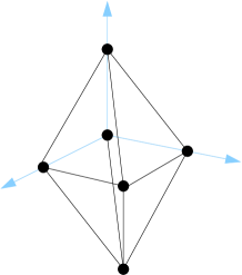
Figure 4: Toric diagram for the $k=(1,1,-1,-1)$ theory.

We now repeat the analysis for $k=(1,1,-1,-1)$. In this case, we quotient by $Q_{1}+Q_{3}$ and $Q_{1}+Q_{4}$, which gives

$$Q_{D(1,1,-1,-1)}=\left(\begin{array}[]{cccccc}0&-1&1&1&-1&0\\ \ \ 1&\ \ 0&\ \ -1&\ \ -1&\ \ 0&\ \ 1\end{array}\right)$$ (4.13)

Once again, the $SU(2)^{3}\times U(1)$ symmetry is clear from this matrix. The doublets are now different from the previous case, and are given by $(A_{1},C_{2})$, $(A_{2},C_{1})$ and $(B_{1},B_{2})$. Taking the kernel we obtain

$$G^{T}_{(1,1,-1,-1)}=\left(\begin{array}[]{cccccc}\ \ -1&\ \ 0&\ \ 0&\ \ 0&\ \ 0&\ \ 1\\ 0&-1&0&0&1&0\\ 1&1&0&1&0&0\\ 1&1&0&0&0&0\end{array}\right)$$ (4.14)

It is straightforward to see that it also corresponds to the toric diagram in Figure 4.

Let us provide some argument of why this theory does not come from a (3+1)d parent. From Figure 3, we see that the quiver contains nodes with a single incoming and a single outgoing arrow. Such nodes correspond to $N_{f}=N_{c}$ gauge groups and possibly generate dynamical scales, not leading to a CFT.

5 A Klebanov-Witten RG flow

Using crystals, the authors of [35] have proposed some Klebanov-Witten type RG flows [32] connecting theories, which result from adding adjoint masses. The adjoint masses come from twisting bonds in the crystal. In particular, it is suggested there should exist such a flow between $C(dP_{3})\times\mathbb{C}$ and $C(Q^{111})$. We now investigate this flow and use it to determine the gauge theory for $C(dP_{3})\times\mathbb{C}$. We go a step beyond [35] and propose the quiver for this model, which is shown in (5). It is obtained by undoing the RG flow that we now explain.

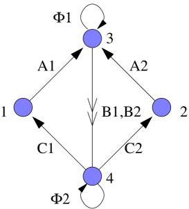
Figure 5: Quiver diagram for $C(dP_{3})\times\mathbb{C}$.

The superpotential is

$$W=\phi_{1}(B_{1}C_{1}A_{1}-B_{2}C_{2}A_{2})-\phi_{2}(C_{1}A_{1}B_{1}-C_{2}A_{2}B_{2})~{}.$$ (5.15)

The RG flow is triggered by the following mass term

$$\Delta W=-(\phi_{1}^{2}-\phi_{2}^{2}).$$ (5.16)

It is straightforward to verify that, by integrating out the massive fields $\phi_{1}$ and $\phi_{2}$, we recover (4.9) up to an unimportant overall multiplicative constant. This is indeed very encouraging. Let us now check that the theory with quiver diagram in Figure 5 and superpotential (5.15) has $C(dP_{3})\times\mathbb{C}$ as its moduli space for some choice of CS levels. As before, it is a straightforward exercise to write down the matrix translating quiver fields to GLSM fields. It is given by

$$P=\left(\begin{array}[]{c|cccccccccc}&\ \ p_{1}&\ \ p_{2}&\ \ p_{3}&\ \ p_{4}&\ \ p_{5}&\ \ p_{6}&\ \ p_{7}&\ \ p_{8}&\ \ p_{9}&\ \ p_{10}\\ \hline\cr A_{1}&1&1&1&0&0&0&0&0&0&0\\ A_{2}&1&0&0&1&0&0&1&0&0&0\\ B_{1}&0&0&0&1&1&1&0&0&0&0\\ B_{2}&0&1&0&0&1&0&0&1&0&0\\ C_{1}&0&0&0&0&0&0&1&1&1&0\\ C_{2}&0&0&1&0&0&1&0&0&1&0\\ \phi_{1}&0&0&0&0&0&0&0&0&0&1\\ \phi_{2}&0&0&0&0&0&0&0&0&0&1\end{array}\right)$$ (5.17)

This determines the charge matrix $Q_{F}=Ker(P)$ encoding the F-term equations.

$$Q_{F}=\left(\begin{array}[]{cccccccccc}\ \ p_{1}&\ \ p_{2}&\ \ p_{3}&\ \ p_{4}&\ \ p_{5}&\ \ p_{6}&\ \ p_{7}&\ \ p_{8}&\ \ p_{9}&\ \ p_{10}\\ \hline\cr 1&0&-1&0&0&0&-1&0&1&0\\ 1&-1&0&0&0&0&-1&1&0&0\\ 1&0&-1&-1&0&1&0&0&0&0\\ 1&-1&0&-1&1&0&0&0&0&0\end{array}\right)$$ (5.18)

From (5.17), we can determine how GLSM fields are charged under the four quiver $U(1)$’s. This is given by

$$\begin{array}[]{c|cccccccccc}&\ \ p_{1}&\ \ p_{2}&\ \ p_{3}&\ \ p_{4}&\ \ p_{5}&\ \ p_{6}&\ \ p_{7}&\ \ p_{8}&\ \ p_{9}&\ \ p_{10}\\ \hline\cr Q_{1}&1&0&0&0&0&0&-1&0&0&0\\ Q_{2}&0&0&0&0&0&0&1&0&-1&0\\ Q_{3}&-1&0&0&0&1&0&0&0&0&0\\ Q_{4}&0&0&0&0&-1&0&0&0&1&0\end{array}$$ (5.19)

Since the CS levels are not affected by the RG flow, once again we are interested in looking at the theory with $k=(1,1,-1,-1)$. This tells us that we can impose the D-terms for $Q_{1}+Q_{3}$ and $Q_{1}+Q_{4}$.

$$Q_{D}=\left(\begin{array}[]{cccccccccc}\ \ p_{1}&\ \ p_{2}&\ \ p_{3}&\ \ p_{4}&\ \ p_{5}&\ \ p_{6}&\ \ p_{7}&\ \ p_{8}&\ \ p_{9}&\ \ p_{10}\\ \hline\cr 0&0&0&0&1&0&-1&0&0&0\\ 1&0&0&0&-1&0&-1&0&1&0\end{array}\right)$$ (5.20)

The total charge matrix is obtained from concatenating (5.18) and (5.20). The toric diagram is again given by

$$G^{T}=Ker(Q_{tot})=\left(\begin{array}[]{cccccccccc}\ \ p_{1}&\ \ p_{2}&\ \ p_{3}&\ \ p_{4}&\ \ p_{5}&\ \ p_{6}&\ \ p_{7}&\ \ p_{8}&\ \ p_{9}&\ \ p_{10}\\ \hline\cr 0&0&0&0&0&0&0&0&0&1\\ -1&-1&0&0&0&1&0&0&1&0\\ 0&1&0&-1&0&-1&0&1&0&0\\ 2&1&1&2&1&1&1&0&0&0\end{array}\right)$$ (5.21)

The result is represented in Figure 6, where we use the first three rows of the previous matrix. This is indeed the toric diagram for $C(dP_{3})\times\mathbb{C}$.

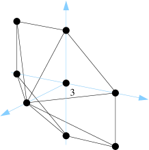
Figure 6: Toric diagram for the $k=(1,1,-1,-1)$ theory.

The multiplicity of GLSM fields in Figure 6 does not project down to any of the toric diagrams that arise from $dP_{3}$ quivers [39]. We also know this is the case because, otherwise, the gauge theory would have six gauge groups and a completely different quiver. Like $C(Q^{111})$ this is a pure (2+1)d theory.

6 More examples

6.1 Another pair of theories connected by an RG flow

We now present a similar pair of theories connected by an RG flow, also anticipated in [34]. The two theories correspond to $D_{3}$ and $\mathbb{C}^{3}/(\mathbb{Z}_{2}\times\mathbb{Z}_{2})\times\mathbb{C}$. Crystal model suggest that the superpotential of the theories corresponding to $\mathbb{C}^{3}/(\mathbb{Z}_{2}\times\mathbb{Z}_{2})\times\mathbb{C}$ are the same as those of $C(dP_{3})\times\mathbb{C}$ in the abelian limit (namely when fields are no longer matrices and ordering becomes unimportant). I.e., nodes in both crystals combine the same fields. This hints that the matter contents are related by suitable flips of the charges. We expect $D_{3}$ and $C(Q^{111})$ to be connected in a similar way.

Let us first consider $D_{3}$. Its quiver is shown in Figure 7. It is obtained from the $C(Q^{111})$ quiver by flipping half of the arrows. The superpotential is

$$W=C_{1}A_{1}B_{1}B_{2}A_{2}C_{2}-B_{1}C_{1}A_{1}A_{2}C_{2}B_{2}~{}.$$ (6.22)

This superpotential follows form crystal models and, as we explained, can be obtained from the superpotential of $C(Q^{111})$ by changing the order of fields according to the charge assignments.

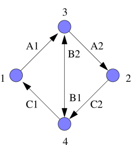
Figure 7: Quiver diagram for $D_{3}$.

Since we have only two superpotential terms, $Q_{F}=0$, as for $Q^{111}$, and GLSM fields are identified with chiral fields. The quiver $U(1)$ charges are given by

$$\begin{array}[]{r|cccccccc}&A_{1}&C_{1}&A_{2}&C_{2}&B_{1}&B_{2}\\ \hline\cr Q_{1}&1&-1&0&0&0&0\\ Q_{2}&0&0&-1&1&0&0\\ Q_{3}&-1&0&1&0&1&-1\\ Q_{4}&0&1&0&-1&-1&1\end{array}$$ (6.23)

As for $Q^{111}$, there are two choices of CS levels that produce the desired moduli space: $k=(1,1,-1,-1)$ and $k=(1,-1,0,0)$. We analyze $k=(1,1,-1,-1)$, the other option is analogous. We quotient by $Q_{1}+Q_{3}$ and $Q_{1}+Q_{4}$, given by the matrix

$$Q_{D}=\left(\begin{array}[]{cccccc}0&-1&1&0&1&-1\\ \ \ 1&\ \ 0&\ \ 0&\ \ -1&\ \ -1&\ \ 1\\ \end{array}\right)$$ (6.24)

In this case, $Q_{tot}=Q_{D}$. Its kernel determines the toric diagram matrix

$$G^{T}=\left(\begin{array}[]{cccccc}\ \ -1&\ \ -1&\ \ 0&\ \ 0&\ \ 0&\ \ 1\\ 1&1&0&0&1&0\\ 1&0&0&1&0&0\\ 0&1&1&0&0&0\end{array}\right)$$ (6.25)

This matrix corresponds to the toric diagram for $D_{3}$. Figure 8 plots its last three rows.

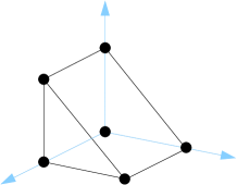
Figure 8: Toric diagram for the $k=(1,1,-1,-1)$ theory.

In passing, we note that it is easy to identify another theory whose moduli space is $D_{3}$. It arises from the (3+1)d parent theory of the cone over the Suspended Pinch Point(SPP), whose toric diagram can be obtained from that of $D_{3}$ by a suitable projection. In this case, the gauge theory has only three gauge groups [45] and the CS couplings are $k=(1,-1,0)$, with zero in one of the gauge groups without the adjoint [43]. This example shows a behavior that we expect to be generic, the same moduli space arises from theories with and without (3+1)d parents. Furthermore, these theories can have a different number of gauge groups.

We now propose a theory for $\mathbb{C}^{3}/(\mathbb{Z}_{2}\times\mathbb{Z}_{2})\times\mathbb{C}$. We obtain its quiver from the one of $C(dP_{3})\times\mathbb{C}$, shown in Figure 5, by flipping the direction of $A_{2}$, $B_{2}$ and $C_{2}$. The quiver diagram is shown in Figure 9.

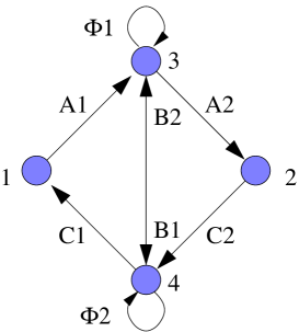
Figure 9: Quiver diagram for $\mathbb{C}^{3}/(\mathbb{Z}_{2}\times\mathbb{Z}_{2})\times\mathbb{C}$.

The superpotential is

$$W=\phi_{1}(B_{1}C_{1}A_{1}-A_{2}C_{2}B_{2})+\phi_{2}(B_{2}A_{2}C_{2}-C_{1}A_{1}B_{1})$$ (6.26)

As explained before, the superpotential of $\mathbb{C}^{3}/(\mathbb{Z}_{2}\times\mathbb{Z}_{2})\times\mathbb{C}$ is the same as $C(dP_{3})\times\mathbb{C}$ in the abelian case. Because of this, the $P$ and $Q_{F}$ matrices as are the same of $C(dP_{3})\times\mathbb{C}$, (5.17) and (5.18). The quiver $U(1)$ charges correspond to

$$\begin{array}[]{r|cccccccccccc}&p_{1}&p_{2}&p_{3}&p_{4}&p_{5}&p_{6}&p_{7}&p_{8}&p_{9}&p_{10}\\ \hline\cr Q_{1}&0&0&1&1&0&-1&-1&0&0&0\\ Q_{2}&0&-1&1&0&0&0&-1&1&0&0\\ Q_{3}&0&-1&0&1&0&0&0&0&0&0\\ Q_{4}&0&0&0&0&0&-1&0&1&0&0\end{array}$$ (6.27)

Let us consider $k=(1,1,-1,-1)$ (once again, $k=(1,-1,0,0)$ gives the same moduli space). We then consider $Q_{1}+Q_{3}$ and $Q_{1}+Q_{4}$, which give

0-1120-1-100000110-2-1100)subscript𝑄𝐷fragments 0-1120-1-1000fragments00110-2-1100Q_{D}=\left(\begin{tabular}[]{cccccccccc}$p_{1}$&$p_{2}$&$p_{3}$&$p_{4}$&$p_{5}$&$p_{6}$&$p_{7}$&$p_{8}$&$p_{9}$&$p_{10}$\cr\hline\cr 0&-1&1&2&0&-1&-1&0&0&0\cr 0&0&1&1&0&-2&-1&1&0&0\end{tabular}\right)

p1p2p3p4p5p6p7p8p9p10p1p2p3p4p5p6p7p8p9p10 (6.28)

Combining $Q_{F}$ and $Q_{D}$ and finding its kernel, we get

1010-10101000-11101100011011-10000000000001).superscript𝐺𝑇𝐾𝑒𝑟subscript𝑄𝑡𝑜𝑡fragments 1010-10101000-11101100011011-10000000000001G^{T}=Ker(Q_{tot})=\left(\begin{tabular}[]{cccccccccc}$p_{1}$&$p_{2}$&$p_{3}$&$p_{4}$&$p_{5}$&$p_{6}$&$p_{7}$&$p_{8}$&$p_{9}$&$p_{10}$\cr\hline\cr 1&0&1&0&-1&0&1&0&1&0\cr 0&0&-1&1&1&0&1&1&0&0\cr 0&1&1&0&1&1&-1&0&0&0\cr 0&0&0&0&0&0&0&0&0&1\end{tabular}\right).

p1p2p3p4p5p6p7p8p9p10p1p2p3p4p5p6p7p8p9p10 (6.29)

Removing, for example, the first row gives the toric diagram of $\mathbb{C}^{3}/(\mathbb{Z}_{2}\times\mathbb{Z}_{2})\times\mathbb{C}$ as shown in Figure 10.

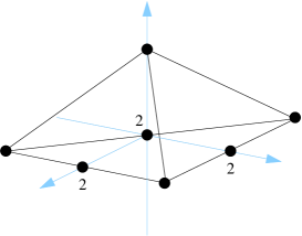
Figure 10: Toric diagram for the $k=(1,1,-1,-1)$ theory.

There is a further check we can perform on the two theories we have just introduced. In [35], it is suggested that there exists an Klebanov-Witten type RG-flow connecting $\mathbb{C}^{3}/(\mathbb{Z}_{2}\times\mathbb{Z}_{2})\times\mathbb{C}$ and $D_{3}$ theories. Indeed, it is easy to check that adding $(\phi_{2}^{2}-\phi_{1}^{2})$ to (6.26) and integrating out the massive fields, we obtain (6.22).

6.2 $\mathbb{C}^{3}/(\mathbb{Z}_{N}\times\mathbb{Z}_{N})\times\mathbb{C}$ orbifold

We can extend our results for $\mathbb{C}^{3}/(\mathbb{Z}_{2}\times\mathbb{Z}_{2})\times\mathbb{C}$ and give a proposal for a general $\mathbb{C}^{3}/(\mathbb{Z}_{N}\times\mathbb{Z}_{N})\times\mathbb{C}$ orbifold. The theory contains $2N$ gauge groups and $4N$ matter fields given by

$$\begin{array}[]{ccc}X_{i}&&(\raisebox{-0.5pt}{\hbox{\rule{0.4pt}{6.5pt}\hskip-0.4pt\rule{6.5pt}{0.4pt}\hskip-6.5pt\rule[6.5pt]{6.5pt}{0.4pt}}\rule[6.5pt]{0.4pt}{0.4pt}\hskip-0.4pt\rule{0.4pt}{6.5pt}}_{2(i-1)},\overline{\raisebox{-0.5pt}{\hbox{\rule{0.4pt}{6.5pt}\hskip-0.4pt\rule{6.5pt}{0.4pt}\hskip-6.5pt\rule[6.5pt]{6.5pt}{0.4pt}}\rule[6.5pt]{0.4pt}{0.4pt}\hskip-0.4pt\rule{0.4pt}{6.5pt}}}_{2i-1})\\ Y_{i}&&(\raisebox{-0.5pt}{\hbox{\rule{0.4pt}{6.5pt}\hskip-0.4pt\rule{6.5pt}{0.4pt}\hskip-6.5pt\rule[6.5pt]{6.5pt}{0.4pt}}\rule[6.5pt]{0.4pt}{0.4pt}\hskip-0.4pt\rule{0.4pt}{6.5pt}}_{2i-1},\overline{\raisebox{-0.5pt}{\hbox{\rule{0.4pt}{6.5pt}\hskip-0.4pt\rule{6.5pt}{0.4pt}\hskip-6.5pt\rule[6.5pt]{6.5pt}{0.4pt}}\rule[6.5pt]{0.4pt}{0.4pt}\hskip-0.4pt\rule{0.4pt}{6.5pt}}}_{2i})\\ Z_{i}&&(\raisebox{-0.5pt}{\hbox{\rule{0.4pt}{6.5pt}\hskip-0.4pt\rule{6.5pt}{0.4pt}\hskip-6.5pt\rule[6.5pt]{6.5pt}{0.4pt}}\rule[6.5pt]{0.4pt}{0.4pt}\hskip-0.4pt\rule{0.4pt}{6.5pt}}_{2i},\overline{\raisebox{-0.5pt}{\hbox{\rule{0.4pt}{6.5pt}\hskip-0.4pt\rule{6.5pt}{0.4pt}\hskip-6.5pt\rule[6.5pt]{6.5pt}{0.4pt}}\rule[6.5pt]{0.4pt}{0.4pt}\hskip-0.4pt\rule{0.4pt}{6.5pt}}}_{2(i-1)})\\ \phi_{i}&&\mbox{Adj}_{2i}\end{array}$$ (6.30)

with $i=1,\ldots,N$ and nodes in the quiver identified by $\mod(2N)$. The superpotential is

$$W=\sum_{i=1}^{N}\phi_{i}(X_{i+1}Y_{i+1}Z_{i+1}-Z_{i}X_{i}Y_{i})~{}.$$ (6.31)

From this superpotential, we can use Kasteleyn matrix techniques to determine that the number of GLSM fields is $3^{N}+1$. Because of this, it is computationally difficult to verify this proposal for large $N$. In Appendix A, we confirm it explicitly for $N=3$. The notation in the previous section for $\mathbb{C}^{3}/(\mathbb{Z}_{2}\times\mathbb{Z}_{2})\times\mathbb{C}$ translates into the general notation as follows: $(A_{1},A_{2},B_{1},B_{2},C_{1},C_{2})\to(Y_{1},X_{1},Z_{1},Z_{2},Y_{2},X_{2})$ and nodes are relabeled according to $(1,2,3,4)\to(1,3,2,4)$.

It is interesting to consider the $N=1$ case, since it provides an alternative to ABJM for M2-branes on $\mathbb{C}^{4}$. The model has a $U(N_{1})\times U(N_{2})$ gauge group with $X$ transforming as $(N_{2},\bar{N}_{1})$, $Y$ as $(N_{1},\bar{N}_{2})$ and two adjoints $\phi_{1}$ and $Z=\phi_{2}$ of $U(N_{2})$. The superpotential is given by

$$W=\phi_{1}\,X\,Y\,\phi_{2}-\phi_{2}\,X\,Y\,\phi_{1}~{}.$$ (6.32)

The moduli space is $\mathbb{C}^{4}$ for CS levels $(1,-1)$. See [43] for the same theory, but derived by other methods. It would be interesting to understand how supersymmetry is enhanced in this model.

7 Partial resolution

7.1 Partial resolution in CS theories

Different geometries and their dual gauge theories can be connected by partial resolution. Partial resolution works in this case very similarly to (3+1)d, with a few new features that we now discuss.

We can turn on FI parameters for any of the gauge groups, with the consequent modification of the D-term equations. The $G-2$ ones that originally vanish are of most importance. As a result of the FI terms, some chiral fields in the quiver (equivalently the corresponding GLSM fields) acquire vevs. These vevs higgs the theory at low energies and can also give mass to some of the chiral fields, which have to be integrated out.

It is interesting to notice that for the specific case of manifolds of the form CY${}_{3}\times\mathbb{C}$, the number of possible partial resolutions is smaller than for CY₃. The reason for this is twofold. The CY${}_{3}\times\mathbb{C}$ theory has generally less gauge groups than the CY₃ counterpart and only $G-2$ independent FI terms result in resolutions.

We also need to take care of the CS couplings. As we now show, whenever two gauge groups are higgsed to the diagonal subgroup by a bifundamental vev, the resulting CS coupling is the sum of the original ones. Suppose some field with charges $(-1,1)$ under gauge groups ${\cal A}^{1}$ and ${\cal A}^{2}$, whose CS couplings are $k_{1}$ and $k_{2}$, acquires a vev. For its scalar component, the covariant derivative is

$$D_{\mu}\Phi=\partial_{\mu}\Phi-i({\cal A}^{1}_{\mu}-{\cal A}^{2}_{\mu})\Phi\ ~{}.$$ (7.33)

The combination ${\cal A}^{-}_{\mu}={\cal A}^{1}_{\mu}-{\cal A}^{2}_{\mu}$ becomes massive. We call $m$ its mass. The relevant piece of the action is

$$S=\int d^{3}x\,k_{1}\epsilon^{\mu\nu\rho}{\cal A}^{1}_{\mu}\partial_{\nu}{\cal A}^{1}_{\rho}+k_{2}\epsilon^{\mu\nu\rho}{\cal A}^{2}_{\mu}\partial_{\nu}{\cal A}^{2}_{\rho}-m^{2}({\cal A}_{\mu}^{1}-{\cal A}_{\mu}^{2})^{2}+\cdots\ .$$ (7.34)

Defining ${\cal A}^{\pm}={\cal A}^{1}\pm{\cal A}^{2}$ and $k_{\pm}=k_{1}\pm k_{2}$, we get

$$S=\int d^{3}x\,k_{+}\epsilon^{\mu\nu\rho}{\cal A}^{+}_{\mu}\partial_{\nu}{\cal A}^{+}_{\rho}+k_{+}\epsilon^{\mu\nu\rho}{\cal A}^{-}_{\mu}\partial_{\nu}{\cal A}^{-}_{\rho}+2k_{-}\epsilon^{\mu\nu\rho}{\cal A}^{-}_{\mu}\partial_{\nu}{\cal A}^{+}_{\rho}-m^{2}({\cal A}^{-}_{\mu})^{2}+\cdots\ .$$ (7.35)

At energies well below $m$, we can proceed to integrate out ${\cal A}^{-}$. The equation of motion reads

$$k_{-}\epsilon^{\mu\nu\rho}\partial_{\nu}{\cal A}^{+}_{\rho}+k_{+}\epsilon^{\mu\nu\rho}\partial_{\nu}{\cal A}^{-}_{\rho}=m^{2}{\cal A}_{\mu}^{-}~{}.$$ (7.36)

At energies well below $m$, we can consider ${\cal A}^{-}$ is constant. Then, the previous expression reduces to

$$k_{-}\epsilon^{\mu\nu\rho}\partial_{\nu}{\cal A}^{+}_{\rho}\sim m^{2}{\cal A}_{\mu}^{-}$$ (7.37)

and

$$S\sim\int d^{3}x\,k_{+}\epsilon^{\mu\nu\rho}{\cal A}^{+}_{\mu}\partial_{\nu}{\cal A}^{+}_{\rho}+2k_{-}\epsilon^{\mu\nu\rho}{\cal A}^{-}_{\mu}\partial_{\nu}{\cal A}^{+}_{\rho}-m^{2}({\cal A}^{-}_{\mu})^{2}+\cdots\ .$$ (7.38)

Plugging the approximate solution to the equation of motion we get

$$S=\int d^{3}x\,k_{+}\epsilon^{\mu\nu\rho}{\cal A}^{+}_{\mu}\partial_{\nu}{\cal A}^{+}_{\rho}-\frac{k_{-}^{2}}{2m^{2}}F_{\mu\nu}^{+}F_{\mu\nu}^{+}\cdots\ .$$ (7.39)

As anticipated, we get a CS coupling for the surviving gauge field whose CS level is the sum of the Higgsed CS levels. In addition, there is a Maxwell term that vanishes in the IR limit (equivalently in the $m\to\infty$ limit).

7.2 Connections between models

We now investigate the web of connections that result from partial resolutions between the theories we have studied. With this goal in mind, the list of partial resolutions we considered is certainly not exhaustive.

By now, we expect the reader to be familiar with the kind of matrices that arise when analyzing these models from a toric geometry perspective. Hence, for the brevity of the presentation, we just state the quiver vevs that are turned on (working out the corresponding vevs for GLSM fields is straightforward) and the results.

$\mathbb{C}^{3}/(\mathbb{Z}_{3}\times\mathbb{Z}_{3})\times\mathbb{C}$ is resolved down to $\mathbb{C}^{3}/(\mathbb{Z}_{2}\times\mathbb{Z}_{2})\times\mathbb{C}$ by turning on vevs for $X_{1}$ and $Z_{1}$. The CS levels match the ones we have studied. $\mathbb{C}^{3}/(\mathbb{Z}_{2}\times\mathbb{Z}_{2})\times\mathbb{C}$ can be resolved to $C(T^{11})\times\mathbb{C}$ by vevs of $A_{1}$ and $A_{2}$. The quiver diagram is shown in Figure 11.a, $k=(1,-1)$ and the superpotential is

$$W=\phi_{1}(B_{1}C_{1}-C_{2}B_{2})+\phi_{2}(B_{2}C_{2}-C_{1}B_{1})~{}.$$ (7.40)

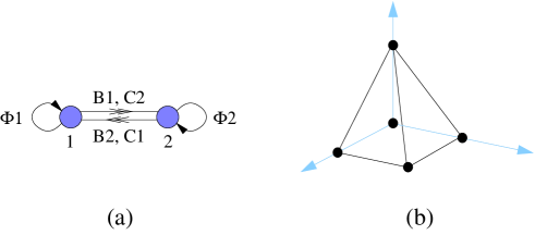
Figure 11: Quiver and toric diagram for $C(T^{11})\times\mathbb{C}$.

This theory has been recently discussed in [29]. On the other hand, turning on a vev for $B_{1}$ resolves $\mathbb{C}^{3}/(\mathbb{Z}_{2}\times\mathbb{Z}_{2})\times\mathbb{C}$ down to $C(SPP)\times\mathbb{C}$. This is a new gauge theory without a (3+1)d parent. Its quiver diagram is shown in Figure 12.a, $k=(1,-2,1)$ and its superpotential is given by

$$W=\phi_{1}(C_{1}A_{1}-A_{2}C_{2}B_{2})+\phi_{2}(B_{2}A_{2}C_{2}-C_{1}A_{1})~{}.$$ (7.41)

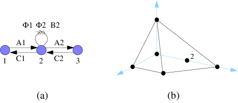
Figure 12: Quiver and toric diagram for $C(SPP)\times\mathbb{C}$.

This is in agreement with the crystal proposal [35]. Computing its moduli space, we obtain the toric diagram in Figure 12.b.

$C(dP_{3})\times\mathbb{C}$ has a very similar pair of resolutions to the same theories. Vevs for $A_{1}$ and $A_{2}$ take us to $C(T^{11})\times\mathbb{C}$, and a vev for $B_{1}$ takes us to $C(SPP)\times\mathbb{C}$.

In summary, we have been able to connect all the theories we have discussed in this paper by either partial resolutions or mass deformations. Figure 13 summarizes the “roadmap” of connections between the models.

\psfrag{Z3 x Z3}[cc][.5]{$\mathbb{C}^{3}/(\mathbb{Z}_{3}\times\mathbb{Z}_{3})\times\mathbb{C}$}\psfrag{Z2 x Z2}[cc][.5]{$\mathbb{C}^{3}/(\mathbb{Z}_{2}\times\mathbb{Z}_{2})\times\mathbb{C}$}\psfrag{conifold}[cc][.6]{$C(T^{11})\times\mathbb{C}$}\psfrag{SPP}[cc][.6]{$C(SPP)\times\mathbb{C}$}\psfrag{Q111}[cc][.6]{$C(Q^{111})\times\mathbb{C}$}\psfrag{D3}[cc][.6]{$D_{3}$}\psfrag{dP3}[cc][.6]{$C(dP_{3})\times\mathbb{C}$}\includegraphics[width=284.52756pt]{roadmap.eps}

Figure 13: Connections between the theories we have studied. PR indicates partial resolution and “mass” corresponds to RG flows following mass deformations.

8 Conclusions

In this paper we have constructed various examples of (2+1)d ${\cal N}=2$ CS gauge theories that do not have a (3+1)d origin. One of them is the gauge theory for $C(Q^{111})$. We have also considered KW-type RG-flows connecting different theories as well as partial resolutions. It turns out that the chiral field content, superpotentials, RG-flows and partial resolutions are in agreement with crystal models. It is important to emphasize, though, that all our computations, most notably the calculation of moduli spaces, are independent of the validity of crystal models. Thus, our results can be regarded as new evidence that crystal models indeed capture the structure of these theories.

An ambitious goal would be to obtain an efficient procedure for constructing the (2+1)d CS gauge theory for an arbitrary toric CY₄-fold, analogous to the one provided by dimer models in (3+1)d. To do this, it is still necessary to understand crystal models in more detail, in particular how they encode gauge groups. The helical path idea of [43] seems to be a promising direction. A robust proof of the correspondence between crystal models and CY₄/CFT₃ is desirable. It is conceivable that the correspondence can be proved both with string theory methods like [46] or purely in field theoretic terms as in [44].

The next step would be to determine all gauge theories whose moduli space is a given geometry. Then, we can investigate whether these models are related by some kind of duality. An interesting Seiberg duality for CS theories has been recently introduced in [47]. The full set of dualities might be larger than this since, in general, we expect dual models can have different number of gauge groups. We have briefly mentioned this possibility in section 6.1, for the case of $D_{3}$. Interestingly, (2+1)d mirror symmetry is rich in such examples [48]. The $D_{3}$ models are also examples of theories with and without (3+1)d parents having the same moduli space. A similar pair is the ABJM model and the $N=1$ case of the models in section 6.2.

Understanding how geometry translates into field theory is the first step towards a general understanding of AdS₄/CFT₃ in ${\cal N}=2$ settings. In addition, we would like to perform various checks on the dual pairs. One such test, is the precision matching of R-charges computed from field theory and geometry as done in (3+1)d [24]. At this moment, it is not clear how to implement such program. While the computation can be done on the geometric side using the techniques in [41], it is still not known how to use the field theory ideas of [49] in this context. Another possibility is to work out the BPS operators on both sides of the correspondence, along the lines of [50]. This program has been already initiated in the context of M2-branes in [52, 29, 43]. We believe that plenty of new structures are still waiting to be discovered and we hope to report our progress in the near future.

Acknowledgements

We would like to thank Y.-H. He, C. Herzog, S. Lee, G. Torroba and specially I. Klebanov and A. Zaffaroni for useful discussions. S.F. is supported by the DOE under contract DE-FG02-91ER-40671 and by the National Science Foundation under Grant No. PHY05-51164. D. R-G. acknowledges financial support from the European Commission through Marie Curie OIF grant contract no. MOIF-CT- 2006-38381. J.P. is supported in part by the KOSEF SRC Program through CQUeST at Sogang University, by KOSEF Grant R01-2008-000-20370-0 and by the Stanford Institute for Theoretical Physics.

Appendix A $\mathbb{C}^{3}/(\mathbb{Z}_{3}\times\mathbb{Z}_{3})\times\mathbb{C}$

In this appendix, we investigate the general proposal of the section 6.2 for the case of $N=3$ The quiver diagram is shown in Figure 14. The superpotential is

$$W=\phi_{1}(X_{2}Y_{2}Z_{2}-Z_{1}X_{1}Y_{1})+\phi_{2}(X_{3}Y_{3}Z_{3}-Z_{2}X_{2}Y_{2})+\phi_{3}(X_{1}Y_{1}Z_{1}-Z_{3}X_{3}Y_{3})~{}.$$ (A.42)

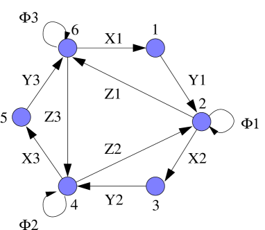
Figure 14: Quiver diagram for $\mathbb{C}^{3}/(\mathbb{Z}_{3}\times\mathbb{Z}_{3})\times\mathbb{C}$.

From this superpotential, we can construct the following Kasteleyn matrix. Rows and columns correspond to negative and positive superpotential terms, respectively

$$K=\left(\begin{array}[]{ccc}\phi_{1}&0&X_{1}+Y_{1}+Z_{1}\\ X_{2}+Y_{2}+Z_{2}&\phi_{2}&0\\ 0&X_{3}+Y_{3}+Z_{3}&\phi_{3}\end{array}\right)$$ (A.43)

The GLSM fields (perfect matchings of the crystal) can be computed as $\det K$. Notice that although we are using technology that is borrowed from the study of dimer models, the reasoning above is independent of any dimer model interpretation and applies to any theory in which the superpotential satisfies the toric condition (i.e. that every field appears in exactly two terms, with opposite signs). They are 28, and their relation to quiver fields is encoded in the following matrix

$$P=\left(\begin{array}[]{c|cccccccccccccccccccccccccccc}&p_{1}&p_{2}&p_{3}&p_{4}&p_{5}&p_{6}&p_{7}&p_{8}&p_{9}&p_{10}&p_{11}&p_{12}&p_{13}&p_{14}&p_{15}&p_{16}&p_{17}&p_{18}&p_{19}&p_{20}&p_{21}&p_{22}&p_{23}&p_{24}&p_{25}&p_{26}&p_{27}&p_{28}\\ X_{1}&1&0&1&0&1&0&1&0&0&0&0&0&1&0&1&0&0&0&1&0&1&0&0&0&1&0&0&0\\ X_{2}&1&1&0&0&1&1&0&0&1&0&1&0&0&0&0&0&0&0&1&1&0&0&1&0&0&0&0&0\\ X_{3}&1&1&1&1&0&0&0&0&1&1&0&0&1&1&0&0&1&0&0&0&0&0&0&0&0&0&0&0\\ Z_{1}&0&1&0&1&0&1&0&1&0&0&0&0&0&1&0&1&0&0&0&1&0&1&0&0&0&1&0&0\\ Z_{2}&0&0&1&1&0&0&1&1&0&1&0&1&0&0&0&0&0&0&0&0&1&1&0&1&0&0&0&0\\ Z_{3}&0&0&0&0&1&1&1&1&0&0&1&1&0&0&1&1&0&1&0&0&0&0&0&0&0&0&0&0\\ Y_{1}&0&0&0&0&0&0&0&0&1&1&1&1&0&0&0&0&1&1&0&0&0&0&1&1&0&0&1&0\\ Y_{2}&0&0&0&0&0&0&0&0&0&0&0&0&1&1&1&1&1&1&0&0&0&0&0&0&1&1&1&0\\ Y_{3}&0&0&0&0&0&0&0&0&0&0&0&0&0&0&0&0&0&0&1&1&1&1&1&1&1&1&1&0\\ \phi_{1}&0&0&0&0&0&0&0&0&0&0&0&0&0&0&0&0&0&0&0&0&0&0&0&0&0&0&0&1\\ \phi_{2}&0&0&0&0&0&0&0&0&0&0&0&0&0&0&0&0&0&0&0&0&0&0&0&0&0&0&0&1\\ \phi_{3}&0&0&0&0&0&0&0&0&0&0&0&0&0&0&0&0&0&0&0&0&0&0&0&0&0&0&0&1\end{array}\right).$$ (A.44)

$Q_{F}$ is the $20\times 28$ dimensional matrix obtained as $Ker(P)$. We do not exhibit here for space reasons. The quiver $U(1)$ charges can be reproduced by the following charge matrix

$$\begin{array}[]{c|cccccccccccccccccccccccccccc}&p_{1}&p_{2}&p_{3}&p_{4}&p_{5}&p_{6}&p_{7}&p_{8}&p_{9}&p_{10}&p_{11}&p_{12}&p_{13}&p_{14}&p_{15}&p_{16}&p_{17}&p_{18}&p_{19}&p_{20}&p_{21}&p_{22}&p_{23}&p_{24}&p_{25}&p_{26}&p_{27}&p_{28}\\ \hline\cr Q_{1}&-1&0&0&0&0&0&0&0&1&0&0&0&0&0&0&0&0&0&0&0&0&0&0&0&0&0&0&0\\ Q_{2}&0&1&0&0&0&0&0&0&0&-1&0&0&0&0&0&0&0&0&0&0&0&0&0&0&0&0&0&0\\ Q_{3}&0&-1&0&0&0&0&0&0&0&0&0&0&0&1&0&0&0&0&0&0&0&0&0&0&0&0&0&0\\ Q_{4}&0&0&1&0&0&0&0&0&0&0&0&0&0&0&-1&0&0&0&0&0&0&0&0&0&0&0&0&0\\ Q_{5}&0&-1&0&0&0&0&0&0&0&0&0&0&0&0&0&0&0&0&0&1&0&0&0&0&0&0&0&0\\ Q_{6}&1&1&-1&0&0&0&0&0&-1&1&0&0&0&-1&1&0&0&0&0&-1&0&0&0&0&0&0&0&0\end{array}$$ (A.45)

Following the general proposal, we take CS levels $k=(1,-1,1,-1,1,-1)$. We then quotient by $Q_{1}+Q_{2}$, $Q_{1}+Q_{4}$, $Q_{1}+Q_{6}$ and $Q_{2}+Q_{3}$. Then, we have

$$Q_{D}=\left(\begin{array}[]{cccccccccccccccccccccccccccc}p_{1}&p_{2}&p_{3}&p_{4}&p_{5}&p_{6}&p_{7}&p_{8}&p_{9}&p_{10}&p_{11}&p_{12}&p_{13}&p_{14}&p_{15}&p_{16}&p_{17}&p_{18}&p_{19}&p_{20}&p_{21}&p_{22}&p_{23}&p_{24}&p_{25}&p_{26}&p_{27}&p_{28}\\ \hline\cr-1&1&0&0&0&0&0&0&1&-1&0&0&0&0&0&0&0&0&0&0&0&0&0&0&0&0&0&0\\ -1&0&1&0&0&0&0&0&1&0&0&0&0&0&-1&0&0&0&0&0&0&0&0&0&0&0&0&0\\ 0&1&-1&0&0&0&0&0&0&1&0&0&0&-1&1&0&0&0&0&-1&0&0&0&0&0&0&0&0\\ 0&0&0&0&0&0&0&0&0&-1&0&0&0&1&0&0&0&0&0&0&0&0&0&0&0&0&0&0\end{array}\right)$$ (A.46)

We combine $Q_{F}$ and $Q_{D}$ into $Q_{tot}$ and calculate the toric diagram of the moduli space as $G^{T}=Ker(Q_{tot})$. The result is

$$G^{T}=\left(\begin{array}[]{cccccccccccccccccccccccccccc}p_{1}&p_{2}&p_{3}&p_{4}&p_{5}&p_{6}&p_{7}&p_{8}&p_{9}&p_{10}&p_{11}&p_{12}&p_{13}&p_{14}&p_{15}&p_{16}&p_{17}&p_{18}&p_{19}&p_{20}&p_{21}&p_{22}&p_{23}&p_{24}&p_{25}&p_{26}&p_{27}&p_{28}\\ \hline\cr 0&0&0&0&0&0&0&0&0&0&0&0&0&0&0&0&0&0&0&0&0&0&0&0&0&0&0&1\\ -2&-2&-2&-2&-2&-2&-2&-2&-1&-1&-1&-1&-1&-1&-1&-1&0&0&-1&-1&-1&-1&0&0&0&0&1&0\\ 0&1&1&2&1&2&2&3&0&1&1&2&0&1&1&2&0&1&0&1&1&2&0&1&0&1&0&0\\ 3&2&2&1&2&1&1&0&2&1&1&0&2&1&1&0&1&0&2&1&1&0&1&0&1&0&0&0\end{array}\right)$$ (A.47)

In Figure 15 we plot the first three rows of this matrix. This corresponds precisely to the toric diagram of $\mathbb{C}^{3}/(\mathbb{Z}_{3}\times\mathbb{Z}_{3})\times\mathbb{C}$ and has a nice structure of multiplicities.

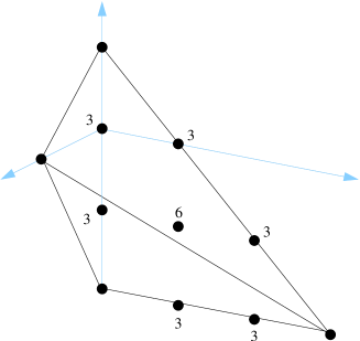
Figure 15: Toric diagram for the $k=(1,-1,1,-1,1,-1)$ theory.

Appendix B Parity invariance

Parity invariance is a key property expected to be satisfied by M2-brane theories. In this appendix we present some evidence that our models preserve parity invariance. More concretely, we show that when we expand the action around a point in moduli space at which gauge groups with opposite CS levels are higgsed to the diagonal subgroup, parity invariance is preserved up to irrelevant terms (for some assumption about the superpotential). Our method is similar to the one used in [51] to derive the action of D2-branes from that of M2-branes.

In order to illustrate our strategy, let us consider the toy model shown in Figure 16. The gauge group is $U(N_{1})\times U(N_{2})$ and we have two bifundamentals $X_{12}$, $X_{21}$ and one adjoint $\Phi$ for the second group. This theory contains various structures that are present in general models.

\psfrag{X12}[cc][1]{$X_{12}$}\psfrag{X21}[cc][1]{$X_{21}$}\includegraphics[width=113.81102pt]{quiver_toy_parity.eps}

Figure 16: A toy model we use to investigate our ideas about parity invariance.

The action is given by

$$S = \frac{1}{2}\int d^{3}x(-D_{\mu}X_{12}D^{\mu}X_{12}^{\dagger}-D_{\mu}X_{21}D^{\mu}X_{21}^{\dagger}-D_{\mu}\Phi D^{\mu}\Phi)$$ (B.48)

$$+ \frac{k}{2}\int d^{3}x\epsilon^{\mu\nu\lambda}({\cal A}^{1}_{\mu}\partial_{\nu}{\cal A}^{1}_{\lambda}+\frac{2i}{3}{\cal A}^{1}_{\mu}{\cal A}^{1}_{\nu}{\cal A}^{1}_{\lambda}-{\cal A}^{2}_{\mu}\partial_{\nu}{\cal A}^{2}_{\lambda}-\frac{2i}{3}{\cal A}^{2}_{\mu}{\cal A}^{2}_{\nu}{\cal A}^{2}_{\lambda})+\ldots$$

where the covariant derivatives are

$$D_{\mu}X_{12} = \partial_{\mu}X_{1}+i({\cal A}^{1}_{\mu}X_{12}-X_{12}{\cal A}^{2}_{\mu})$$

$$D_{\mu}X_{21} = \partial_{\mu}X_{2}+i({\cal A}^{2}_{\mu}X_{21}-X_{21}{\cal A}^{1}_{\mu})$$

$$D_{\mu}\Phi = \partial_{\mu}\Phi+i[{\cal A}^{2}_{\mu},\Phi]$$ (B.49)

with $\Phi$ being Hermitian. We leave traces implicit in all our expressions. Next, let us define the combinations

$$2{\cal A}^{\pm}={\cal A}^{1}\pm{\cal A}^{2}~{}.$$ (B.50)

The CS term can be rewritten as follows

$$\epsilon^{\mu\nu\lambda}({\cal A}^{1}_{\mu}\partial_{\nu}{\cal A}^{1}_{\lambda}-{\cal A}^{2}_{\mu}\partial_{\nu}{\cal A}^{2}_{\lambda}) = 4\epsilon^{\mu\nu\lambda}{\cal A}^{-}_{\mu}\partial_{\nu}{\cal A}^{+}_{\lambda}$$

$$\epsilon^{\mu\nu\lambda}({\cal A}^{1}_{\mu}{\cal A}^{1}_{\nu}{\cal A}^{1}_{\lambda}-{\cal A}^{2}_{\mu}{\cal A}^{2}_{\nu}{\cal A}^{2}_{\lambda}) = 2\epsilon^{\mu\nu\lambda}({\cal A}^{-}_{\mu}{\cal A}^{-}_{\nu}{\cal A}^{-}_{\lambda}+3{\cal A}^{-}_{\mu}{\cal A}^{+}_{\nu}{\cal A}^{+}_{\lambda})~{}.$$ (B.51)

We can also write

$$\begin{array}[]{rcl}D_{\mu}X_{12}&=&\partial_{\mu}X_{1}+i[{\cal A}^{+},X_{12}]+i({\cal A}^{-}_{\mu}X_{12}+X_{12}{\cal A}^{-}_{\mu})\\ &\equiv&D^{+}_{\mu}X_{12}+i({\cal A}^{-}_{\mu}X_{12}+X_{12}{\cal A}^{-}_{\mu})\\ \\ D_{\mu}X_{12}^{\dagger}&=&\partial_{\mu}X_{12}^{\dagger}+i[{\cal A}^{+},X_{12}^{\dagger}]+i({\cal A}^{-}_{\mu}X_{12}^{\dagger}+X_{12}^{\dagger}{\cal A}^{-}_{\mu})\\ &\equiv&D^{+}_{\mu}X_{12}^{\dagger}+i({\cal A}^{-}_{\mu}X_{12}^{\dagger}+X_{12}^{\dagger}{\cal A}^{-}_{\mu})\end{array}$$ (B.52)

Next, let us expand around some point in moduli space $X_{12}=R\,{\bf 1}_{N\times N}$ such that $X_{12}=R\,{\bf 1}_{N\times N}+\tilde{X}_{12}$.

$$\begin{array}[]{rcl}D_{\mu}X_{12}D^{\mu}X_{12}^{\dagger}&=&D^{+}_{\mu}\tilde{X}_{12}D^{+\mu}\tilde{X}_{12}^{\dagger}+{\cal A}^{-}_{\mu}{\cal A}^{-\mu}(R^{2}+{\cal O}(\tilde{X}_{12}^{2}))\\ &+&i(2R{\cal A}^{-}_{\mu}+{\cal A}^{-}_{\mu}\tilde{X}_{12}+\tilde{X}_{12}{\cal A}^{-}_{\mu})D^{+\mu}\tilde{X}_{12}^{\dagger}\\ &-&i(2R{\cal A}^{-}_{\mu}+{\cal A}^{-}_{\mu}\tilde{X}_{12}^{\dagger}+\tilde{X}_{12}^{\dagger}{\cal A}^{-}_{\mu})D^{+\mu}\tilde{X}_{12}\\ \\ D_{\mu}X_{21}D^{\mu}X_{21}^{\dagger}&=&D^{+}_{\mu}X_{21}D^{+\mu}X_{21}^{\dagger}+i({\cal A}^{-}_{\mu}X_{21}+X_{21}{\cal A}^{-}_{\mu})D^{+\mu}X_{21}^{\dagger}\\ &-&i({\cal A}^{-}_{\mu}X_{21}^{\dagger}+X_{21}^{\dagger}{\cal A}^{-}_{\mu})D^{+\mu}X_{21}\\ \\ (D_{\mu}\Phi)^{2}&=&(D^{+}_{\mu}\Phi)^{2}-2i[{\cal A}^{-}_{\mu},\Phi]D^{+}_{\mu}\Phi-([{\cal A}^{-}_{\mu},\Phi])^{2}\end{array}$$ (B.53)

The action does not contain any derivative of ${\cal A}^{-}_{\mu}$. Then, similarly to [51], we can eliminate it from the action using its equation of motion, resulting in

$$S = \frac{1}{2}\int d^{3}x(-D^{+}_{\mu}\tilde{X}_{12}D^{+\mu}\tilde{X}_{12}^{\dagger}-D^{+}_{\mu}X_{21}D^{+\mu}X_{21}^{\dagger}-D^{+}_{\mu}\Phi D^{+\mu}\Phi$$ (B.54)

$$\frac{1}{4(R^{2}+{\cal O}(\tilde{X}_{12}^{2},X_{21}^{2},\Phi^{2}))}G_{\mu}G^{\mu}+i{\cal A}^{-}_{\mu}{\cal A}^{-}_{\nu}{\cal A}^{-}_{\lambda})+\ldots$$

We are indeed integrating out ${\cal A}^{-}_{\mu}$. The last term should be understood as a shorthand for what results from replacing ${\cal A}^{-}$ by the equation of motion. We have also defined

$$G^{\mu} = 4k\epsilon^{\mu\nu\lambda}D^{+}_{\nu}{\cal A}^{+}_{\lambda}+2iRD^{+\mu}X_{12}^{\dagger}-2iRD^{+\mu}X_{12}$$ (B.55)

$$+ \sum_{i=\{12,21\}}(2iX_{i}D^{+\mu}X_{i}^{\dagger}-2iX_{i}^{\dagger}D^{\mu}X_{i}+2iD^{+\mu}X_{i}^{\dagger}X_{i}-2iD^{+\mu}X_{i}X_{i}^{\dagger}$$

$$-2i[,\Phi]D^{+\mu}\Phi)~{}.$$

Starting from the previous equation, we drop the tilde in $\tilde{X}_{12}$. The $D^{+}_{\nu}{\cal A}^{+}_{\lambda}$ squared term gives the usual YM kinetic term. The commutator term in the last line of (B.55) comes from $[{\cal A}^{-}_{\mu},\Phi]D^{+\mu}\Phi$ in the action, from which we have extracted ${\cal A}^{-}_{\mu}$. Componentwise, the last line involves the structure constants $f^{abc}$ of the Lie algebra. $R$ plays the role of a perturbation expansion parameter. If the superpotential is quartic (say with terms of the form $X_{12}X_{21}\Phi^{2}$) ${\cal A}^{+}_{\lambda}$, $X_{i}$ and $\Phi$ have canonical dimension $1/2$.

Parity acts by, for example, $x_{1}\rightarrow-x_{1}$. We can make (B.55) invariant if $X_{i}\rightarrow X_{i}^{\dagger}$ and $\Phi$ does not change under a parity transformation. Notice that $X_{i}\rightarrow X_{i}^{\dagger}$ is the same type of transformation used in ABJM to achieve parity invariance [12]. In ABJM, this operation is accompanied by exchanging the two gauge groups. In our notation, flipping the gauge groups corresponds to ${\cal A}^{-}_{\mu}\to-{\cal A}^{-}_{\mu}$. Since we have integrated out ${\cal A}^{-}_{\mu}$, this last transformation is not visible in our formalism.

Terms involving $\Phi$ are irrelevant. So is the $({\cal A}^{-})^{3}$ term after using the equation of motion. Thus, the parity violating terms vanish in the IR limit. We expect this kind of argument can be applied to generic points in moduli space. We can regard the procedure we have just outlined as going to some kind of unitary gauge. The method is a bit subtle, since the transformation is singular when $(R^{2}+{\cal O}(X_{i}^{2},\Phi^{2}))$ vanishes. Our arguments are based on the chiral fields having dimension $1/2$. This issue becomes more subtle for sextic superpotentials, but we have already seen that models with sextic superpotential such as $C(Q^{111})$ can be regarded as models with a quartic superpotential by adding massive adjoints.

This method can be applied to most of the models in our paper, in which we can separate gauge groups into pairs with $(k,-k)$ CS levels. Let us, for example, consider the $C(Q^{111})$ theory. We have

$$S = -\frac{1}{2}\int(D_{\mu}A_{i}D^{\mu}A_{i}^{\dagger}+D_{\mu}B_{i}D^{\mu}B_{i}^{\dagger}+D_{\mu}C_{i}D^{\mu}C_{i}^{\dagger})$$ (B.56)

$$+ \frac{k}{2}\int\epsilon^{\mu\nu\lambda}({\cal A}_{1}\partial_{\nu}{\cal A}_{1}-{\cal A}_{3}\partial_{\nu}{\cal A}_{3}+{\cal A}_{2}\partial_{\nu}{\cal A}_{2}-{\cal A}_{4}\partial_{\nu}{\cal A}_{4})+\cdots$$

and

$$D_{\mu}A_{1} = \partial_{\mu}A_{1}+i({\cal A}_{1}-{\cal A}_{3})A_{1}$$

$$D_{\mu}C_{2} = \partial_{\mu}C_{2}+i({\cal A}_{4}-{\cal A}_{2})C_{2}~{}.$$ (B.57)

Proceeding as before, we can rewrite the CS term as

$$\epsilon^{\mu\nu\lambda}(({\cal A}_{1}-{\cal A}_{3})_{\mu}\partial_{\nu}({\cal A}_{1}+{\cal A}_{3})_{\lambda}+({\cal A}_{2}-{\cal A}_{4})_{\mu}\partial_{\nu}({\cal A}_{2}+{\cal A}_{4})_{\lambda}).$$ (B.58)

Expanding around $A_{1}=R$ and $C_{2}=r$, we can integrate out the $({\cal A}_{1}-{\cal A}_{3})$ and $({\cal A}_{2}-{\cal A}_{4})$ combinations. Then, we see parity invariance can be achieved by $A_{i},B_{i},C_{i}\rightarrow A_{i}^{\dagger},B_{i}^{\dagger},C_{i}^{\dagger}$ up to irrelevant terms.

References

• [1] J. M. Maldacena, “The large N limit of superconformal field theories and supergravity,” Adv. Theor. Math. Phys.  2, 231 (1998) [Int. J. Theor. Phys.  38, 1113 (1999)] [arXiv:hep-th/9711200].
• [2] S. S. Gubser, I. R. Klebanov and A. M. Polyakov, “Gauge theory correlators from non-critical string theory,” Phys. Lett.  B 428, 105 (1998) [arXiv:hep-th/9802109].
• [3] E. Witten, “Anti-de Sitter space and holography,” Adv. Theor. Math. Phys.  2, 253 (1998) [arXiv:hep-th/9802150].
• [4] J. H. Schwarz, “Superconformal Chern-Simons theories,” JHEP 0411 (2004) 078 [arXiv:hep-th/0411077].
• [5] J. Bagger and N. Lambert, “Modeling multiple M2’s,” Phys. Rev.  D 75 (2007) 045020 [arXiv:hep-th/0611108].
• [6] J. Bagger and N. Lambert, “Gauge Symmetry and Supersymmetry of Multiple M2-Branes,” Phys. Rev.  D 77 (2008) 065008 [arXiv:0711.0955 [hep-th]].
• [7] J. Bagger and N. Lambert, “Comments On Multiple M2-branes,” JHEP 0802 (2008) 105 [arXiv:0712.3738 [hep-th]].
• [8] A. Gustavsson, “Algebraic structures on parallel M2-branes,” arXiv:0709.1260 [hep-th].
• [9] A. Gustavsson, “Selfdual strings and loop space Nahm equations,” arXiv:0802.3456 [hep-th].
• [10] M. Van Raamsdonk, “Comments on the Bagger-Lambert theory and multiple M2-branes,” arXiv:0803.3803 [hep-th].
• [11] N. Lambert and D. Tong, “Membranes on an Orbifold,” Phys. Rev. Lett.  101, 041602 (2008) [arXiv:0804.1114 [hep-th]].
• [12] O. Aharony, O. Bergman, D. L. Jafferis and J. Maldacena, “N=6 superconformal Chern-Simons-matter theories, M2-branes and their gravity duals,” arXiv:0806.1218 [hep-th].
• [13] D. Gaiotto and E. Witten, “Janus Configurations, Chern-Simons Couplings, And The Theta-Angle in N=4 Super Yang-Mills Theory,” arXiv:0804.2907 [hep-th].
• [14] K. Hosomichi, K. M. Lee, S. Lee, S. Lee and J. Park, “N=4 Superconformal Chern-Simons Theories with Hyper and Twisted Hyper Multiplets,” arXiv:0805.3662 [hep-th].
• [15] K. Hosomichi, K.M. Lee, S. Lee, S. Lee and J. Park, “ ${\cal N}=5,6$ superconformal Chern-Simons theories and M2-branes on orbifolds,” arXiv:0806.4977 [hep-th].
• [16] M. Benna, I. Klebanov, T. Klose and M. Smedback, “Superconformal Chern-Simons Theories and AdS4/CFT3 Correspondence,” arXiv:0806.1519 [hep-th].
• [17] M. Schnabl and Y. Tachikawa, “ Classification of ${\cal N}=6$ superconformal theories of ABJM type,” arXiv:0807.1102 [hep-th].
• [18] E. A. Bergshoeff, O. Hohm, D. Roest, H. Samtleben and E. Sezgin, “ The superconformal gaugings in three dimensions,” arXiv:0807.2841 [hep-th].
• [19] J. Bagger and N. Lambert, “ Three-algebras and ${\cal N}=6$ Chern-Simons gauge theorie,” arXiv:0807.0163 [hep-th].
• [20] D. L. Jafferis and A. Tomasiello, “ A simple class of ${\cal N}=3$ gauge/gravity duals,” arXiv:0808.0864 [hep-th].
• [21] J. Bhattacharya and S. Minwalla, “Superconformal indices for ${\cal N}=6$ Chern-Simons theories,” arXiv:0806.3251 [hep-th].
• [22] K. Hosomichi, K. M. Lee, S. Lee, S. Lee, J. Park and P. Yi, “A Nonperturbative Test of M2-Brane Theory,” arXiv:0809.1771 [hep-th].
• [23] Y. Imamura and K. Kimura, “N=4 Chern-Simons theories with auxiliary vector multiplets,” arXiv:0807.2144 [hep-th] ; Y. Imamura, K. Kimura “On the moduli space of elliptic Maxwell-Chern-Simons theories,” arXiv:0806.3727 [hep-th].
• [24] S. Benvenuti , S. Franco, A. Hanany , D. Martelli and J. Sparks, “An Infinite family of superconformal quiver gauge theories with Sasaki-Einstein duals,” JHEP 0506 (2005) 064, hep-th/0411264.
• [25] A. Hanany and K. D. Kennaway, arXiv:hep-th/0503149.
• [26] S. Franco, A. Hanany , K. Kennaway, D. Vegh and B. Wecht, “Brane dimers and quiver gauge theories,” JHEP 0601 (2006) 096, hep-th/0504110.
• [27] S. Franco, A. Hanany , D. Martelli , J. Sparks , D. Vegh and B. Wecht “Gauge theories from toric geometry and brane tilings,” JHEP 0601 (2006) 128, hep-th/0505211.
• [28] D. Martelli and J. Sparks, “ Moduli spaces of Chern-Simons quiver gauge theories,” arXiv:0808.0912 [hep-th].
• [29] A. Hanany and A. Zaffaroni, “ Tilings, Chern-Simons theories and M2 branes,” arXiv:0808.1244 [hep-th].
• [30] K. Ueda and M. Yamazaki, “ Toric Calabi-Yau four-folds dual to Chern-Simons-matter theories,” arXiv:0808.3768 [hep-th].
• [31] Y. Imamura and K. Kimura, “Quiver Chern-Simons theories and crystals,” arXiv:0808.4155 [hep-th].
• [32] I. R. Klebanov and E. Witten, “Superconformal field theory on threebranes at a Calabi-Yau singularity,” Nucl. Phys.  B 536(1998) 199 [arXiv:hep-th/9807080].
• [33] S. Lee, “Superconformal field theories from crystal lattices,” Phys. Rev.  D 75 (2007) 101901 [arXiv:hep-th/0610204].
• [34] S. Lee, S. Lee and J. Park, “Toric AdS(4)/CFT(3) duals and M-theory crystals,” JHEP 0705(2007) 004 [arXiv:hep-th/0702120]
• [35] S. Kim, S. Lee, S. Lee and J. Park, “Abelian Gauge Theory on M2-brane and Toric Duality,” Nucl. Phys.  B 797 (2008) 340 [arXiv:0705.3540 [hep-th]].
• [36] B. Feng, A. Hanany and Y. H. He, “D-brane gauge theories from toric singularities and toric duality,” Nucl. Phys.  B 595, 165 (2001) [arXiv:hep-th/0003085].
• [37] B. Feng, A. Hanany, Y. H. He and A. M. Uranga, “Toric duality as Seiberg duality and brane diamonds,” JHEP 0112, 035 (2001) [arXiv:hep-th/0109063].
• [38] D. Forcella, A. Hanany, Y. H. He and A. Zaffaroni, “Mastering the Master Space,” arXiv:0801.3477 [hep-th].
D. Forcella, A. Hanany, Y. H. He and A. Zaffaroni, “The Master Space of N=1 Gauge Theories,” JHEP 0808, 012 (2008) [arXiv:0801.1585 [hep-th]].
• [39] B. Feng, S. Franco, A. Hanany and Y. H. He, “Symmetries of toric duality,” JHEP 0212, 076 (2002) [arXiv:hep-th/0205144].
• [40] P. S. Aspinwall, B. R. Greene and D. R. Morrison, “Calabi-Yau moduli space, mirror manifolds and spacetime topology change in string theory,” Nucl. Phys.  B 416, 414 (1994) [arXiv:hep-th/9309097].
• [41] D. Martelli, J. Sparks and S. T. Yau, “The geometric dual of a-maximisation for toric Sasaki-Einstein manifolds,” Commun. Math. Phys.  268, 39 (2006) [arXiv:hep-th/0503183].
• [42] D. Martelli, J. Sparks and S. T. Yau, “Sasaki-Einstein manifolds and volume minimisation,” Commun. Math. Phys.  280, 611 (2008) [arXiv:hep-th/0603021].
• [43] A. Hanany, D. Vegh and A. Zaffaroni, “Brane Tilings and M2 Branes,” arXiv:0809.1440 [hep-th].
• [44] S. Franco and D. Vegh, “Moduli spaces of gauge theories from dimer models: Proof of the correspondence,” JHEP 0611, 054 (2006) [arXiv:hep-th/0601063].
• [45] D. R. Morrison and M. R. Plesser, “Non-spherical horizons. I,” Adv. Theor. Math. Phys.  3, 1 (1999) [arXiv:hep-th/9810201].
• [46] B. Feng, Y. H. He, K. D. Kennaway and C. Vafa, “Dimer models from mirror symmetry and quivering amoebae,” arXiv:hep-th/0511287.
• [47] A. Giveon and D. Kutasov, “Seiberg Duality in Chern-Simons Theory,” arXiv:0808.0360 [hep-th].
• [48] K. A. Intriligator and N. Seiberg, “Mirror symmetry in three dimensional gauge theories,” Phys. Lett.  B 387, 513 (1996) [arXiv:hep-th/9607207].
• [49] E. Barnes, E. Gorbatov, K. A. Intriligator, M. Sudano and J. Wright, “The exact superconformal R-symmetry minimizes tau(RR),” Nucl. Phys.  B 730, 210 (2005) [arXiv:hep-th/0507137].
• [50] B. Feng , A. Hanany and Y. He, “Counting gauge invariants: The Plethystic program,” JHEP 0703 (2007) 090 hep-th/0701063.
• [51] S. Mukhi and C. Papageorgakis, “M2 to D2,” JHEP 0805, 085 (2008) [arXiv:0803.3218 [hep-th]].
• [52] A. Hanany, N. Mekareeya and A. Zaffaroni, “Partition Functions for Membrane Theories,” arXiv:0806.4212 [hep-th].