Block Density Matrix Renormalization Group with Effective Interactions

Abstract

Based on the contractor renormalization group (CORE) method and the density matrix renormalization group (DMRG) method, a new computational scheme, which is called the block density matrix renormalization group with effective interactions (BDMRG-EI), is proposed to deal with the numerical computation of quantum correlated systems. Different from the convential CORE method in the ways of calculating the blocks and the fragments, where the DMRG method instead of the exact diagonalization is employed in BDMRG-EI, DMRG-EI makes the calculations of larger blocks and fragments applicable. Integrating DMRG’s advantage of high accuracy and CORE’s advantage of low computational costs, BDMRG-EI can be widely used for the theoretical calculations of the ground state and low-lying excited states of large systems with simple or complicated connectivity. Test calculations on a 240 site one-dimensional chain and a double-layer polyacene oligomer containing 48 hexagons demonstrate the efficiency and potentiality of the method.

I Introduction

The real space renormalization group (RSRG) method Wilson75 , firstly proposed by Wilson in 1975, is a variational scheme that can solve large systems through truncating the Hilbert space successively. Despite RSRG’s great success in weakly correlated systems, lots of theoretical calculations have found that it failed for strongly correlated systems.Chui78 ; Bary79 ; Hirsh80 ; Lee79 The breakdown of the RSRG method in the strongly correlated systems is ascribed to its lack of account of the interactions between the blocks, i.e. merely considering isolated blocks in RSRG imposes wrong fixed boundary conditions for the blocks which should actually be in open boundary conditions.White92_0

In order to improve RSRG’s performance for strongly correlated systems, various new schemes have been proposed. These new schemes can be sorted into two types according to their theoretical philosophies. One type focused on searching for new optimal criterion of truncation other than the energy criterion used in the traditional RSRG methods. Among them, the density matrix renormalization group (DMRG) method proposed by White in 1992 White92 ; White93 has been shown as an extremely accurate technique in solving one-dimensional (1D) strongly correlated systems.Schollwock05 The DMRG method projects the wavefunction of a larger block (the superblock) onto the system block and then uses the eigenvalue of the systems block’s reduced density matrix as the basis truncation criterion.

The other type focused on taking into account the influence of discarded excited states in the “isolated” block as an account of the interactions between the blocks, while the energy criterion of truncation is retained.Lepetit93 ; Zivkovic90 ; Morningstar94 ; Morningstar96 ; Weinstein01 ; Capponi04 ; Capponi06 ; Malrieu01 ; Hajj04 ; Hajj04_2 In order to achieve this goal, Lepetit and Manousakis suggested the use of a second-order quasi-degenerate perturbation theory Lepetit93 , and Zivković, et al suggested defining a new transformed Hamiltonian from the calculations on dimers of blocks Zivkovic90 . To formalize the latter idea in a more general way, Morningstar and Weinstein introduced the contractor renormalization group (CORE) method in 1994.Morningstar94 ; Morningstar96 ; Weinstein01 ; Capponi04 ; Capponi06 CORE introduces effective interactions between the blocks from the exact spectrum of dimers or trimers of blocks by virtue of Bloch’s effective Hamiltonian theory Bloch58 . In CORE, the entire system is divided into blocks with even number of sites and several eigenstates are kept in each block. In 2001, Malrieu and Guihéry proposed another new improved version of RSRG - real space renormalization group with effective interactions (RSRG-EI) Malrieu01 ; Hajj04 ; Hajj04_2 . CORE and RSRG-EI originated from similar basic ideas, but RSRG-EI uses larger blocks with odd number of sites and keeps only one eigenstate in each block and RSRG-EI can be applied to infinite systems due to the fact that it is iterative. Because CORE and RSRG-EI divide the whole system into a few blocks and only calculate blocks and fragments with a certain size exactly instead of the whole system, the increase of computational costs is only linearly scaling with the size of the whole system.

Generally, despite of DMRG’s great success in 1D systems, the degeneracy in the reduced density matrix spectrum will increase when DMRG is applied to the quasi-1D large systems with complicated connectivity or two-dimensional (2D) systems, which implies the impractical requirement of much more states to be retained to sustain the numerical precision. In the meantime, although CORE and RSRG-EI are computationally efficient for large systems, the accuracy is a bottleneck due to the limitation in the fragment size that can be solved exactly. Meanwhile, exact or numerically high-precision calculation of larger blocks and fragments is actually very essential to achieve reliable account of the intra-block and inter-block correlation effects, and consequently a reliable account of the total system. In this paper, we propose a new scheme - block density matrix renormalization group with effective interactions (BDMRG-EI), which is a generalization of CORE with the incorporation of DMRG. It combines the advantage of DMRG in accuracy and that of CORE in computational costs.

The outline of the paper is as follows: in Section 2, the details of BDMRG-EI methodology are introduced; in Section 3, demonstrative computations on a 1D chain and a double-layer polyacene oligomers are presented; finally, we conclude and summarize our results in Section 4.

II Methodology

II.1 Bloch’s effective Hamiltonian theory

The one-to-one correspondence between two isodimensional subspaces can be well described by the theory of effective Hamiltonians established by Bloch. Firstly, one may consider a $m$-dimensional model space, onto which one would like to build an effective Hamiltonian $\widehat{H}^{eff}$. Let us call the model space as $S_{0}$ and its projector as $\widehat{P}_{0}$

$$\widehat{P}_{0}=\sum_{I\in S_{0}}|I\rangle\langle I|\qquad I=1,\ldots m$$ (1)

The main task of $\widehat{H}^{eff}$ is to fulfill the requirement that its $m$ eigenvalues are exact eigenvalues and its eigenvectors are the projections of exact eigenvectors in $S_{0}$. This means that if

$$\widehat{H}|\psi_{k}\rangle=\varepsilon_{k}|\psi_{k}\rangle\qquad k=1,\ldots n(n\geq m)$$ (2)

then $\widehat{H}^{eff}$ satisfies the condition that

$$\widehat{H}^{eff}\widehat{P}_{0}|\psi_{k}\rangle=\varepsilon_{k}\widehat{P}_{0}|\psi_{k}\rangle\qquad k=1,\ldots m$$ (3)

The $m$ eigenstates $|\psi_{k}\rangle$ which are targeted by the effective Hamiltonian span the so-called target space $S$, with the projector $\widehat{P}$, isodimensional to $S_{0}$. If the transform operator from $S_{0}$ to $S$ is $\widehat{\Omega}$ ($\widehat{P}=\widehat{\Omega}\widehat{P}_{0}$), then the effective Hamiltonian satisfies Eq. (3) is

$$\widehat{H}^{eff}=\widehat{P}_{0}\widehat{H}\widehat{P}=\widehat{P}_{0}\widehat{\Omega}\widehat{H}\widehat{\Omega}\widehat{P}_{0}$$ (4)

On principle, one may choose $S$ arbitrarily provide that $\widehat{\Omega}$ exists, but an obvious rational choice is to select $m$ eigenstates with largest projections in $S_{0}$ to span $S$, i.e., one should maximize $\sum_{k\in S}\parallel|\widehat{P}_{0}\psi_{k}\rangle\parallel$. After $S$ is constructed, $\widehat{H}^{eff}$ can be obtained from the following equation.

$$\widehat{H}^{eff}=\sum_{k}|\widehat{P}_{0}\psi_{k}\rangle\varepsilon_{k}\langle\widehat{P}_{0}\psi_{k}|$$ (5)

It should be mentioned that, $\widehat{H}^{eff}$ may be non-Hermitian if $|\widehat{P}_{0}\psi_{k}\rangle$ loses the orthogonality after projection, i.e., $\langle\widehat{P}_{0}\psi_{k}|\widehat{P}_{0}\psi_{l}\rangle\neq\delta_{kl}$. Therefore, orthogonalization treatment of $|\widehat{P}_{0}\psi_{k}\rangle$ is necessary before the construction of $\widehat{H}^{eff}$.

II.2 DMRG

Over the last decade, the DMRG method White92 ; White93 has emerged as the most powerful method for the simulation of strongly correlated 1D quantum systems. Here, we would like to give a brief introduction to the main physical principles of DMRG. More technique details can be found in some recent reviews about DMRG Schollwock05 ; Schollwock07 ; Schollwock07_2 .

II.2.1 Decimation of state spaces

Due to the exponential growth of the number of degrees of freedom in quantum many-body systems, the exact simulation in the complete Hilbert space is apparently not feasible beyond very small sizes. Among a great number of various approximate simulation methods for quantum many-body systems, one important class of approximate simulation methods attempts a systematic choice of a subspace of the complete Hilbert space which is anticipated to contain the physically most relevant states. All variational and renormalization group techniques are within this group, and the essential question is of course to identify the best decimation strategy which will depend on both the system and the physical question.

Here, let us particularly focus on the decimation strategy in strongly correlated 1D quantum systems. Imagine we grow the system successively, adding site by site. The original system, which we refer to as an old block, is assumed to be effectively described within a state space ${|\alpha\rangle}$ of dimension $M$, the new site within a state space ${|\sigma\rangle}$ of dimension $N$. Obviously, the state space ${|\beta\rangle}$ of the new block composed of the old block and the newly added site will have the dimension $MN$, and for the prevention of exponential growth it will be decimated down to the dimension $M$. Whatever the physical decimation strategy one uses, the states of the new block will be a linear combination of the old states,

$$|\beta\rangle=\sum_{\alpha}\sum_{\sigma}\langle\alpha\sigma|\beta\rangle|\alpha\rangle|\sigma\rangle\equiv\sum_{\alpha}\sum_{\sigma}A_{\alpha\beta}[\sigma]|\alpha\rangle|\sigma\rangle$$ (6)

where $N$ matrices $A$ of dimension $M\times M$ have been introduced, one for each $|\sigma\rangle$, such that the matrix elements encode the expansion coefficients: $A_{\alpha\beta}[\sigma]=\langle\alpha\sigma|\beta\rangle$. The introduction of the $A$-matrices allows to encode the iterative growth of states of larger and larger blocks by matrix multiplications.

Pushing the above idea further it turns out that, we can generally describe a quantum state of a $L$-site lattice emerging from a decimation procedure as

$$|\psi\rangle=\sum_{\sigma_{1}...\sigma_{L}}A^{1}[\sigma_{1}]A^{2}[\sigma_{2}]...A^{L}[\sigma_{L}]|\sigma_{1}...\sigma_{L}\rangle$$ (7)

Such states are referred to be matrix product states (MPS) Klumper91 ; Fannes92 ; Klumper92 ; Derrida93 ; Ian07 (also known as finitely correlated states). Now, the main problem for simulating the state of a quantum system effectively becomes how we can find suitable $A$-matrices with limited dimensions such that $|\psi\rangle$ approximates the state well. If we want to target the ground state of a Hamiltonian $\widehat{H}$, apparently the optimal choice for the $A$-matrices is to find the prescription yielding those $A$ that minimize $\langle\psi|\widehat{H}|\psi\rangle$ with the constraint of $\langle\psi|\psi\rangle=1$. However, directly working out this expression leads to a highly non-linear expression for the energy in $A$, which is numerically very difficult to be solved. One way to turn the problem low-scaling consists in providing a starting set of $A$-matrices in a warm-up procedure, preferably close to the true solution, and then to repeat the following process iteratively: keeping all $A$-matrices in $|\psi\rangle$ fixed, with only one or two exception(s), and then minimizing $\langle\psi|\widehat{H}|\psi\rangle$ with respect to these one or two flexible $A$-matrix (matrices) and updating these one or two $A$-matrix (matrices) according to the newly determined $|\psi\rangle$ with minimized $\langle\psi|\widehat{H}|\psi\rangle$. After that one shifts the position(s) of the flexible $A$-matrix (matrices) forth and back through the entire chain successively. An optimal approximation of the ground state, which is very close to the real global minimum of $\langle\psi|\widehat{H}|\psi\rangle$, can be gradually reached. Historically, this process corresponds to the so-called finite-system algorithm in standard DMRG language.

II.2.2 DMRG procedures

However, there are still some questions not answered: how can we derive $A$-matrices from the newly determined $|\psi\rangle$ and can we retain all the important information provided by $|\psi\rangle$? Now we will introduce an efficient basis truncation scheme which retains most physically important information and can easily derive new $A$-matrices.

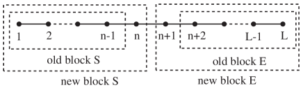
Figure 1: Block definition in DMRG.

Assume we join one block of length $n-1$ and another block with length $L-n-1$ with two active sites explicitly inserted between these two blocks, as illustrated in Fig. 1. In this case, the left block of length $n-1$ would be described by a $M$-dimensional Hilbert space with states ${|m^{S}_{n-1}\rangle}$ which can be described by $A$ matrices as,

$$|m^{S}_{n-1}\rangle=\sum_{\sigma_{1}...\sigma_{n-1}}A^{1}[\sigma_{1}]A^{2}[\sigma_{2}]...A^{L}[\sigma_{n-1}]|\sigma_{1}...\sigma_{n-1}\rangle$$ (8)

Similarly the right block would be described by states ${|m^{E}_{L-n-1}\rangle}$. The left block of length $n-1$ combined with $n$-th site is now called new block S, and the right block of length $L-n-1$ combined with ($n+1$)-th site is now called new block E. So the quantum state of the entire system can be described as,

$$\begin{split}|\psi\rangle&=\sum_{m^{S}=1}^{M}\sum_{\sigma^{S}=1}^{N}\sum_{\sigma^{E}=1}^{N}\sum_{m^{E}=1}^{M}\Psi_{m^{S}m^{E}}[\sigma^{S}\sigma^{E}]|m^{S}\sigma^{S}\rangle|m^{E}\sigma^{E}\rangle\\ &=\sum_{i=1}^{N^{S}}\sum_{j=1}^{N^{E}}\Psi_{ij}|i\rangle|j\rangle\end{split}$$ (9)

where ${|m^{S}\sigma^{S}}\equiv{|i\rangle}$, ${|m^{E}\sigma^{E}}\equiv{|j\rangle}$ and $N^{S}=MN$, $N^{E}=MN$. During the finite-system DMRG sweeps, we shift the positions of the two active sites successively to update all $A$ matrices for improving our wavefunction. In order to prevent the exponential growth of matrix dimension, one has to find a suitable truncation of the basis ${|i\rangle}$ to $M$ states, whose expansion in $|m^{S}\rangle$ and $|\sigma^{S}\rangle$ will just define the desired $A^{n}[\sigma_{n}]$. Similarly, we may also have to find a suitable truncation of the basis ${|j\rangle}$ to $M$ states, whose expansion in $|m^{E}\rangle$ and $|\sigma^{E}\rangle$ will just define the desired $A^{n+1}[\sigma_{n+1}]$.

In order to find the optimal decimation strategy, one can perform Schmidt decomposition for $|\psi\rangle=\sum_{ij}\Psi_{ij}|i\rangle|j\rangle$. After the Schmidt decomposition, one can get the wavefunction in the following new form Schollwock05 :

$$|\psi\rangle=\sum_{\alpha=1}^{N_{Schmidt}}\sqrt{w_{\alpha}}|w^{S}_{\alpha}\rangle|w^{E}_{\alpha}\rangle$$ (10)

where the scalars $w_{\alpha}$ are non-negative, and $|w^{S}_{\alpha}\rangle$ and $|w^{E}_{\alpha}\rangle$ are newly linear recombined vectors with $w_{\alpha}$ for S and E parts respectively. Upon tracing out the E or S part of the state the reduced density matrix for the S or E part is easily found to be

$$\widehat{\rho}_{S}=\sum_{\alpha=1}^{N_{Schmidt}}w_{\alpha}|w^{S}_{\alpha}\rangle\langle w^{S}_{\alpha}|$$ (11)

$$\widehat{\rho}_{E}=\sum_{\alpha=1}^{N_{Schmidt}}w_{\alpha}|w^{E}_{\alpha}\rangle\langle w^{E}_{\alpha}|$$ (12)

Apparently, $w_{\alpha}$ are the eigenvalues of the reduced density matrix for the S or E part.

The approximate wavefunction where the space for S or E part has been truncated to be spanned by only $M$ orthonormal states minimizes the distance to $|\psi\rangle$ if one retains the $M$ eigenstates of $\widehat{\rho}_{S}$ or $\widehat{\rho}_{E}$ with the largest eigenvalues $w_{\alpha}$.Schollwock05 This is just the key truncation criterion in DMRG.

One could also look for a decimation criterion from the view of maximizing the retained biparticle entanglement between S and E parts under truncation. As biparticle entanglement is defined as $S=-\sum_{\alpha}w_{\alpha}log_{2}w_{\alpha}$ and normally one has a large number of relatively small eigenvalues, this again leads to the same truncation prescription: one must retain the $M$ eigenstates of $\widehat{\rho}_{S}$ or $\widehat{\rho}_{E}$ with the largest eigenvalues $w_{\alpha}$. (see e.g. Schollwock05 )

For local quantities, such as energy, magnetization or density, it was also found that the errors are of the order of the truncation weight $\epsilon_{\rho}=1-\sum_{\alpha=1}^{M}w_{\alpha}$, which emerges as the key error estimate.

One can therefore derive $A$-matrices from the effective truncation which retains only $M$ eigenstates of with largest eigenvalues $w_{\alpha}$ of the reduced density matrix built by the newly determined $|\psi\rangle$; in DMRG, the most important information for the purpose of minimizing the errors of the approximate wavefunction and maximizing the retained biparticle entanglement between the blocks is kept if one retains the eigenstates of with largest eigenvalues $w_{\alpha}$ of the reduced density matrix.

Obviously, how efficiently DMRG can work depends on how quickly the ordered eigenvalue spectrum $w_{\alpha}$ of the reduced density matrix $\widehat{\rho}$ will decay. Empirically, in 1D systems, density matrix spectra of gapped quantum systems exhibit roughly system-size independent exponential decay of $w_{\alpha}$. So, DMRG calculations can efficiently yield reliable accuracy that can be comparable to exact calculations for 1D quantum systems if one controls the truncation weight $\epsilon_{\rho}$ very small.

II.3 Block density matrix renormalization group with effective interactions

Similar to that in CORE and RSRG-EI, in BDMRG-EI, the whole system is also divided into a certain number ($N_{block}$) of blocks with sites and only several low-energy states are retained in each block. But in BDMRG-EI, we use DMRG instead of exact diagonization to solve the $m$ lowest eigenstates for each block. For example, $m$ eigenstates $|\Phi(A)_{i}\rangle$ with lowest eigen-energies $\epsilon(A)_{i}$ are obtained for block $A$ with $N_{A}$ sites.

At a later stage, we will derive the effective interactions between the neighbor blocks from the nearly exact spectrum of dimers or trimers of blocks according to Bloch’s effective Hamiltonian theory.

Let me take fragment $A-B$ in the whole system as an example. Fragment $A-B$ contains two blocks: block $A$ and block $B$, and we build small Hilbert spaces spanned by $m$ lowest eigenstates for each block. Then, the model space $S_{0}$ ($dim(S_{0})=m^{2}$) is obtained from the direct product of these two small spaces. The projector of $S_{0}$ is expressed as $\widehat{P}_{0}=\sum_{i=1}^{m^{2}}|\Phi(A-B)_{i}\rangle\langle\Phi(A-B)_{i}|$, where $|\Phi(A-B)_{i}\rangle=|\Phi(A)_{j}\rangle\otimes|\Phi(B)_{k}\rangle$. Then, we perform a standard DMRG calculation for the fragment $A-B$ in oder to get the nearly exact $m^{2}$ low energy eigenstates $|\psi(A-B)_{k}\rangle$ with the energy $\varepsilon(A-B)_{k}$ for the block dimer. Before using Eq. (5) to calculate the the effective Hamiltonian of fragment $A-B$, we should select largest projections on $S_{0}$ to build the target space $S$ and perform orthogonalization treatment of $\widehat{P}_{0}|\psi_{k}\rangle$. ($\widehat{P}_{0}|\psi_{k}\rangle=\sum_{i}|\Phi_{i}\rangle\langle\Phi_{i}|\psi_{k}\rangle$)

According to the above introduction to DMRG, $|\Phi(A)_{i}\rangle$ calculated by DMRG can be described as

$$\begin{split}|\Phi(A)_{i}\rangle=&\sum_{\sigma_{n}}A^{\sigma_{1}}(i)A^{\sigma_{2}}(i)\ldots A^{\sigma_{N_{A}}}(i)\\ &|\sigma_{1}\rangle\otimes|\sigma_{2}\rangle\otimes\ldots|\sigma_{N_{A}}\rangle\end{split}$$ (13)

To enforce the boundary conditions, one may require the leftmost matrix $A^{\sigma_{1}}$ to be $1\times M$-dimensional, and the rightmost matrix $A^{\sigma_{N_{A}}}$ to be $M\times 1$. We can write $|\Phi(B)_{i}\rangle$ and $|\psi(A-B)_{i}\rangle$ similarly.

$$\begin{split}|\Phi(B)_{i}\rangle=&\sum_{\sigma_{n}}B^{\sigma_{N_{A}+1}}(i)B^{\sigma_{NA+2}}(i)\ldots A^{\sigma_{N_{A}+N_{B}}}(i)\\ &|\sigma_{N_{A}+1}\rangle\otimes|\sigma_{N_{A}+2}\rangle\otimes\ldots|\sigma_{N_{A}+N_{B}}\rangle\end{split}$$ (14)

$$\begin{split}|\psi(A-B)_{i}\rangle=&\sum_{\sigma_{n}}C^{\sigma_{1}}(i)C^{\sigma_{2}}(i)\ldots C^{\sigma_{N_{A}+N_{B}}}(i)\\ &|\sigma_{1}\rangle\otimes|\sigma_{2}\rangle\otimes\ldots|\sigma_{N_{A}+N_{B}}\rangle\end{split}$$ (15)

$|\Phi(A-B)_{i}\rangle$ can be expressed as the direct product of $|\Phi(A)_{j}\rangle$ and $|\Phi(B)_{k}\rangle$ as the following equation:

$$\begin{split}|\Phi(A-B)_{i}\rangle=&\sum_{\sigma_{n}}A^{\sigma_{1}}(j)\ldots A^{\sigma_{N_{A}}}(j)\otimes B^{\sigma_{N_{A}+1}}(k)\ldots B^{\sigma_{N_{A}+N_{B}}}(k)\\ &|\sigma_{1}\rangle\otimes|\sigma_{2}\rangle\otimes\ldots|\sigma_{N_{A}+N_{B}}\rangle\end{split}$$ (16)

Therefore, the overlap between DMRG states $|\Phi(A-B)\rangle$ and $|\psi(A-B)\rangle$ can be calculated easily according to the following equation:

$$\begin{split}\langle\Phi|\psi\rangle&=\sum_{\sigma_{n}}(A^{\sigma_{1}*}\ldots A^{\sigma_{N_{A}}*}\otimes B^{\sigma_{N_{A}+1}*}\ldots B^{\sigma_{N_{A}+N_{B}}*})\\ &\text{ }\text{ }\text{ }\text{ }(C^{\sigma_{1}}\ldots C^{\sigma_{N_{A}+N_{B}}})\\ &=E_{N_{A}+N_{B}}\end{split}$$ (17)

where $E_{n}$ can be calculated successively as the following formula:

$$E_{n}=\begin{cases}\sum_{\sigma_{1}}A^{\sigma_{1}*}\otimes C^{\sigma_{1}},&\text{for $n=1$; }\\ \sum_{\sigma_{n}}A^{\sigma_{n}*}E_{n-1}C^{\sigma_{n}},&\text{for $1<n\leq N_{A}$; }\\ \sum_{\sigma_{n}}B^{\sigma_{n}*}\otimes E_{n-1}C^{\sigma_{n}},&\text{for $n=N_{A}+1$; }\\ \sum_{\sigma_{n}}B^{\sigma_{n}*}E_{n-1}C^{\sigma_{n}},&\text{for $N_{A}+1<n\leq N_{A}+N_{B}$. }\end{cases}$$ (18)

When the the overlap between DMRG states can be easily calculated with the above mentioned MPS representations, one can calculate the the effective Hamiltonian of fragment $A-B$ according to Eq. (5).

Similarly, the effective Hamiltonians of other block dimers, trimers or other fragments can also be derived.

After the determination of the the effective Hamiltonian of different fragments, effective interactions between the blocks can be determined by subtracting the contributions of all connected sub-clusters as the following equation.

$$\begin{split}&\widehat{H}^{eff}_{ij}=\widehat{H}^{eff}_{i-j}-\widehat{H}^{eff}_{i}-\widehat{H}^{eff}_{j}\\ &\widehat{H}^{eff}_{ijk}=\widehat{H}^{eff}_{i-j-k}-\widehat{H}^{eff}_{i}-\widehat{H}^{eff}_{j}-\widehat{H}^{eff}_{k}\\ &\text{ }\text{ }\text{ }\text{ }\text{ }\text{ }\text{ }\text{ }\text{ }\text{ }-\widehat{H}^{eff}_{ij}-\widehat{H}^{eff}_{ik}-\widehat{H}^{eff}_{jk}\\ &\ldots\end{split}$$ (19)

Finally, the effective Hamiltonian for the whole system acting on a truncated Hilbert space is obtained through the summation of a series of the local effective Hamiltonians and then directly diagonized with Lanczos or Davidson algorithm.

$$\widehat{H}^{eff}=\sum_{i}\widehat{H}^{eff}_{i}+\sum_{ij}\widehat{H}^{eff}_{ij}+\sum_{ijk}\widehat{H}^{eff}_{ijk}+\ldots$$ (20)

III Test Applications

As a test case of our approach, we have implemented BDMRG-EI calculations to a 240 site 1D chain and a double-layer polyacene (Pac(2)) oligomer containing 48 hexagons within the spin-1/2 Heisenberg model ($H=J\sum_{\langle ij\rangle}S_{i}S_{j}$), where $J$ is a positive exchange constant, and $S_{i}$ represents the spin operator of $i$th site with $\langle ij\rangle$ denoting summation restricted to nearest neighbors. In our test BDMRG-EI calculations, only two lowest eigenstates were kept for each block and only two-body inter-block actions were considered, i.e. $m=2$ and the summation for the whole system’s effective Hamiltonian in Eq. (20) is restricted to the first two terms.

III.1 1D chain

For the 240 site 1D chain, we have four block definition patterns as follow: I. composing of 10 blocks (24 sites in each block); II. composing of 6 blocks (40 sites in each block); III. composing of 4 blocks (60 sites in each block); VI. composing of 3 blocks (80 sites in each block).

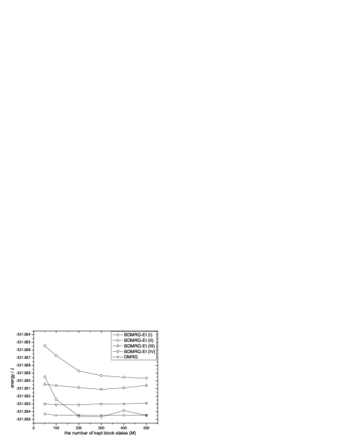
Figure 2: Ground state energy of a 240 site 1D chain.

In Fig. 2, we illustrate the ground state energies calculated by BDMRG-EI and DMRG with different numbers of kept block states ($M$). Obviously, direct diagonalization of the Hamiltonian matrix is impractical at this time for the 240 site 1D Heisenberg chain. Meanwhile, as can be seen in Fig. 2, the DMRG calculated energy has converged with the increase of $M$. Accordingly, this converged value could serve as a reference value for the comparisons of BDMRG-EI results.

As a whole, calculated energies by BDMRG-EI slow down and converge gradually with the increase of $M$, although there are some oscillations, such as the result of BDMRG(I) with $M$=400. This is due to non-variational nature of the BDMRG-EI method. But obviously, the range of the oscillation decreases remarkably with the increase of $M$ and the enlargement of block size.

With large $M$ values, all BDMRG-EI calculations with different block definitions give satisfactory results in good agreement with the DMRG value, with largest error within $0.006J$. This implies that, for 1D systems with simple connectivity, the block size in BDMRG-EI calculations will not affect the ground state results very much.

Figure 3: First excited state energy of a 240 site 1D chain.

In Fig. 3, the calculated energies of first excited state are presented. It can be seen that the errors between the BDMRG-EI results with DMRG standard values for the excited states are much larger than those for the ground state. The values of these errors range from $0.005J$ to around $0.02J$. At the same time, the influence of block size on the computational accuracy are much more significant comparing with that in the case of the ground state. When the block size is too small, BDMRG-EI calculated energies may incorrectly fall below the DMRG result, and smaller block size will lead to larger deviation from the DMRG result. This shows BDMRG-EI’s non-variational nature again. Only when the block size is as large as composed of 60 or 80 sites, BDMRG-EI calculations can give reliable results. These facts elucidated that electrons are much more delocalized in the excited states, which makes it more difficult to evaluate the electron correlation effect in such cases. This implies that incorporation of DMRG into the CORE method is very necessary in calculating the excited states of conjugated systems.

III.2 Double-layer polyacene (Pac(2))

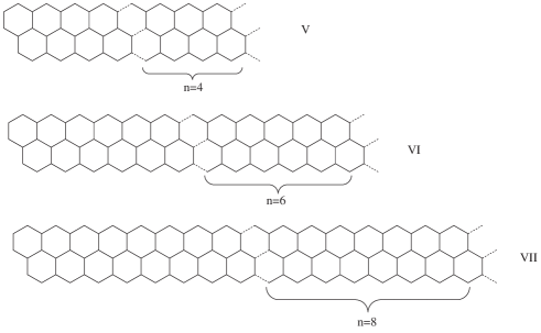
Figure 4: Definitions of blocks for the BDMRG-EI calculation of a Pac(2) oligomer containing 48 hexagons.

The above 1D chain example is a system with simplest connectivity. When the system’s connectivity is more complicated, inter-block correlations will be more significant. As a consequence, the influence of block size on the calculation accuracy will be more remarkable. Here, we take a Pac(2) oligomer containing 48 hexagons as an example. In our BDMRG-EI calculations, three different block definitions are adopted, as shown in Fig. 4.

Figure 5: Ground state energy of a Pac(2) oligomer containing 48 hexagons.

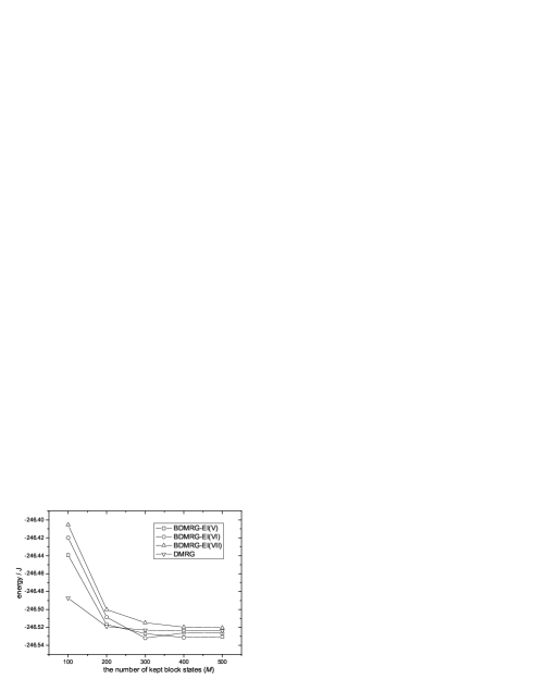
Figure 6: First excited state energy of a Pac(2) oligomer containing 48 hexagons.

Calculated energies of the ground state and the first excited state of this Pac(2) oligomer are shown in Fig. 5 and Fig. 6. Similar to the situation in 1D chain, DMRG calculated values have gradually converged with the increase of $M$ for this Pac(2) oligomer, and the DMRG result with $M=500$ serves as the reference value for comparisons.

In BDMRG-EI calculations with small block sizes, the errors are around $0.2J$ for both the ground state and the first excited state, which are definitely intolerable. However, we can still find from the figures that the results will improve remarkably with the increase of the block size. As an example, the errors in BDMRG-EI(VII) for the ground state and the first excited state fall within $0.05J$. These values are acceptable for such complex system.

It should be mentioned that, even the smallest block size (6-8 hexagons in BDMRG-EI(V)) in BDMRG-EI calculations are far beyond the applicabilities of the normal CORE or RSRG-EI methods(at most 2-3 hexagons).

IV Conclusions

This work proposes BDMRG-EI method as an improvement of the traditional CORE. Within the basic framework of CORE, BDMRG-EI incorporates DMRG calculations into the solution of the blocks and block dimers or trimers.

Our demonstrative calculations showed that the block size effect in systems with complicated connectivity is much more significant than that in systems with simple connectivity, and that in the excited states is also much more significant than that in the ground state. Since the DMRG calculations can achieve high accuracy for systems much larger than those could be exactly treated, BDMRG-EI could take much more intra- and inter-block correlations into account comparing to the original CORE and RSRG-EI methods. Hence, the results of CORE are greatly improved by BDMRG-EI. Demonstrative calculations of a 240 site 1D chain and a Pac(2) oligomer containing 48 hexagons convinced that high accuracy can be achieved in BDMRG-EI calculations when enough large block size is chosen.

Another advantage of BDMRG-EI is its efficiency with low computational costs. Because it solves only the blocks and fragments with a certain size by DMRG instead of the whole system, BDMRG-EI provides a new low-scaling electron structure method which can be applicable to very large systems with simple or complicated connectivity.

References

- (1) K. G. Wilson, Rev. Mod. Phys. 47 (1975), 773.
- (2) S. T. Chui and J. W. Bary, ibid. 18 (1978), 2426.
- (3) S. T. Chui and J. W. Bray, Phys. Rev. B 19 (1979), 4020.
- (4) J. E. Hirsch, ibid. 22 (1980), 5259.
- (5) P. A. Lee, Phys. Rev. Lett. 42 (1979), 1492.
- (6) S. R. White and R. M. Noack, Phys. Rev. Lett. 68 (1992), 3487.
- (7) S. R. White, Phys. Rev. Lett. 69 (1992), 2863.
- (8) S. R. White, Phys. Rev. B 48 (1993), 10345.
- (9) U. Schollwöck, Rev. Mod. Phys. 77 (2005), 259.
- (10) M. B. Lepetit and E. Manousakis, Phys. Rev. B 48 (1993), 1028.
- (11) T. P. Zivković, B. L. Sandleback, T. G. Schmalz, and D. J. Klein, Phys. Rev. B 41 (1990), 2249.
- (12) C. J. Morningstar and M. Weinstein, Phys. Rev. Lett. 73 (1994), 1873.
- (13) C. J. Morningstar and M. Weinstein, Phys. Rev. D 54 (1996), 4131.
- (14) M. Weinstein, Phys. Rev. B 63 (2001), 174421.
- (15) S. Capponi, A. Läuchli and M. Mambrini, Phys. Rev. B 70 (2004), 104424.
- (16) S. Capponi, Theor. Chem. Acc. 116 (2006), 524.
- (17) J. -P. Malrieu and N. Guihéry, Phys. Rev. B 63 (2001), 085110.
- (18) M. A. Hajj, N. Guihéry, J. -P. Malrieu and B. Bocquillon, Eur. Phys. J. B 41 (2004), 11.
- (19) M. Al Hajj, N. Guihéry, J. -P. Malrieu and P. Wind, Phys. Rev. B 70 (2004), 094415.
- (20) C. Bloch, Nucl. Phys. 6 (1958), 329.
- (21) U. Schollwöck, J. Magn. Mag. Mat. 310 (2007), 1394.
- (22) U. Schollwöck, Int. J. Mod. Phys. B 21 (2007), 2564.
- (23) A. Klümper, A. Schadschneider, and J. Zittartz, J. Phys. A: Math. Gen. 24 (1991), L955.
- (24) M. Fannes, B. Nachtergaele, and R. F. Werner, Commun. Math. Phys. 144 (1992), 443.
- (25) A. Klümper, A. Schadschneider, and J. Zittartz, Z. Phys. B 87 (1992), 281.
- (26) B. Derrida, M. R. Evans, V. Hakim, and V. Pasquier, J. Phys. A: Math. Gen. 26 (1993), 1493.
- (27) I. P. McCulloch, J. Stat. Mech. P10014 (2007).