Non-Perturbative Contribution to the Thrust Distribution in $e^{+}e^{-}$ Annihilation

Abstract

We re-evaluate the non-perturbative contribution to the thrust distribution in $e^{+}e^{-}\to$ hadrons, in the light of the latest experimental data and the recent NNLO perturbative calculation of this quantity. By extending the calculation to NNLO+NLL accuracy, we perform the most detailed study to date of the effects of non-perturbative physics on this observable. In particular, we investigate how well a model based on a low-scale QCD effective coupling can account for such effects. We find that the difference between the improved perturbative distribution and the experimental data is consistent with a $1/Q$-dependent non-perturbative shift in the distribution, as predicted by the effective coupling model. Best fit values of $\alpha_{s}\left(91.2\text{ GeV}\right)=0.1164^{+0.0028}_{-0.0026}$ and $\alpha_{0}\left(2\text{ GeV}\right)=0.59\pm 0.03$ are obtained with $\chi^{2}/\text{d.o.f.}=1.09$. This is consistent with NLO+NLL results but the quality of fit is improved. The agreement in $\alpha_{0}$ is non-trivial because a part of the $1/Q$-dependent contribution (the infrared renormalon) is included in the NNLO perturbative correction.

1 Introduction

One of the most common and successful ways of testing QCD has been by investigating the distribution of event shapes in $e^{+}e^{-}\rightarrow$ hadrons, which have been measured accurately over a range of centre-of-mass energies ($14\text{ GeV}\leq Q\leq 207\text{ GeV}$), and provide a useful way of evaluating the strong coupling constant $\alpha_{s}$.

The main obstruction to obtaining an accurate value of $\alpha_{s}$ from these distributions is not due to a lack of precise data but to dominant errors in the theoretical calculation of the distributions. In particular, there are non-perturbative effects that cannot yet be calculated from first principles but cause power-suppressed corrections that can be significant at experimentally accessible energy scales. In the case of the thrust distribution $d\sigma/dT$, previous work has shown that matching $\alpha_{s}$ with a low-scale effective coupling $\alpha_{\text{eff}}$ which extrapolates below some infra-red matching scale $\mu_{I}$ results in a $1/Q$-dependent shift in the distribution that accounts well for the discrepancy between the experimental and perturbative results one .

The presence of $1/Q$ corrections in event shapes is a generic expectation based on the renormalon analysis of perturbation theory, which implies an ambiguity of that order in the perturbative predictions for these observables (see Beneke:1998ui ; Beneke:2000kc for reviews). The low-scale effective coupling hypothesis Dokshitzer:1995qm leads to universality relations between the corrections to different observables, valid to lowest order in the effective coupling, and to a well-defined prescription for matching the perturbative and non-perturbative contributions.

The calculation of Ref. one was performed to NLO+NLL accuracy, i.e. terms up to ${\cal O}\left(\alpha_{s}^{2}\right)$ were retained exactly while exponentiating logarithmically-enhanced terms of the form $\alpha_{s}^{n}\ln^{n+1}(1-T)$ and $\alpha_{s}^{n}\ln^{n}(1-T)$ were summed to all orders. In the present paper, the recent evaluation of the NNLO term (i.e ${\cal O}\left(\alpha_{s}^{3}\right)$) in the fixed-order perturbation series expansion of the thrust distribution two ; three is used to refine the perturbative calculation of the distribution to NNLO+NLL accuracy and thus to reduce the uncertainty present in the theoretical prediction. A low-scale effective coupling is then introduced and matched to NNLO. This is again found to be a good method for dealing with the non-perturbative shift. By comparing the NNLO+NLL+shift results with the latest experimental distributions, values of $\alpha_{s}$ and

$$\alpha_{0}=\frac{1}{\mu_{I}}\int_{0}^{\mu_{I}}d\mu\text{ }\alpha_{\text{eff}}\left(\mu\right)$$ (1)

are obtained. These are consistent with those determined to NLO+NLL accuracy. The agreement is non-trivial because a part of the $1/Q$-dependent contribution – the infrared renormalon – is included in the NNLO perturbative correction.

The organisation of the paper is as follows. In Sect. 2 we briefly recall the relevant properties of the thrust distribution, the fixed-order calculation and the resummation of large logarithms. Sect. 3 presents the predictions of perturbative NNLO+NLL matching and the power dependence of the discrepancy with experimental data. The matching to the low-scale effective coupling and comparisons with data are performed in Sect. 4, and our conclusions are presented in Sect. 5.

2 Perturbative calculation of the thrust distribution

We recall that the thrust $T$ is a measure of the distribution of momenta of the final state hadrons:

$$T=\max_{\overrightarrow{n}}\left(\frac{\sum_{i=1}^{N}\left|\overrightarrow{p_{i}}.\overrightarrow{n}\right|}{\sum_{i=1}^{N}\left|\overrightarrow{p_{i}}\right|}\right),$$ (2)

where $\overrightarrow{n}$ is a unit vector and we sum over the 3-momentum of each final-state hadron in the centre-of-mass frame. Theoretical calculations of thrust are performed by summing over the individual final state partons, as the hadronisation process is still not well understood. $T$ can vary between the limits $T=1$ for back-to-back jets and $T=\frac{1}{2}$ for a uniform angular distribution of hadrons.

For comparison with experiments, it is the thrust distribution

$$\frac{1}{\sigma}\frac{d\sigma}{dT},$$ (3)

which is relevant, where $\sigma$ is the total cross-section for $\text{e}^{+}\text{e}^{-}\rightarrow$ hadrons. In calculations it is more convenient to use the event shape variable

$$t\equiv 1-T,$$ (4)

which has the two-jet limit $t=0$. The distribution away from this limit therefore depends directly upon the production of extra final-state partons at QCD vertices, and hence is ideal for testing QCD and evaluating $\alpha_{s}$. The normalised thrust cross section is then defined as

$$R\left(t\right)=\int_{0}^{t}dt\frac{1}{\sigma}\frac{d\sigma}{dt}=\int_{1-t}^{1}dT\frac{1}{\sigma}\frac{d\sigma}{dT}.$$ (5)

2.1 Fixed-order calculations

The perturbative expansion of the normalised thrust cross section has the general form

$$R(t)=1+\bar{\alpha}_{s}R_{1}(t)+\bar{\alpha}_{s}^{2}R_{2}(t)+\bar{\alpha}_{s}^{3}R_{3}(t)+\ldots,$$ (6)

where $R_{1}\left(t\right)$ is the leading order (LO) coefficient, $R_{2}\left(t\right)$ is the next-to-leading order (NLO) coefficient, $R_{3}\left(t\right)$ is the next-to-next-to-leading order (NNLO) coefficient etc. and $\bar{\alpha}_{s}\equiv\alpha_{s}/2\pi$. Solving the renormalisation group equation for the running coupling to NNLO gives

$$\alpha_{s}\left(\mu_{R}\right) = \frac{2\pi}{\beta_{0}L}\Biggl{(}1-\frac{\beta_{1}\ln L}{\beta_{0}^{2}L}+\frac{1}{\beta_{0}^{2}L^{2}}$$ (7)

$$\left[\frac{\beta_{1}^{2}}{\beta_{0}^{2}}\left(\ln^{2}L-\ln L-1\right)+\frac{\beta_{2}}{\beta_{0}}\right]\Biggr{)},$$

where $\mu_{R}$ is some chosen renormalisation scale (we take $\mu_{R}=Q$ except where stated otherwise),

$$\beta_{0} =\frac{11N-2N_{F}}{6}\;\qquad\beta_{1}=\frac{17N^{2}-5NN_{F}-3C_{F}N_{F}}{6},$$ (8)

$$\beta_{2} =\frac{1}{432}(2857N^{3}+54C_{F}^{2}N_{F}-615NC_{F}N_{F}$$

$$-1415N^{2}N_{F}+66C_{F}N_{F}^{2}+79NN_{F}^{2})\;,$$

with $C_{F}=(N^{2}-1)/2N$ for an SU($N$) gauge theory with $N_{F}$ active flavours ($N=3$ for QCD and $N_{F}=5$ at all energies considered here) and $L=\ln(\mu_{R}^{2}/\Lambda_{\overline{MS}}^{\left(5\right)\text{ }2})$, $\Lambda_{\overline{MS}}^{\left(5\right)}$ being the 5-flavour QCD scale in the modified minimal subtraction renormalisation scheme.

A numerical Monte Carlo program, EERAD3 GehrmannDeRidder:2007jk , has recently been developed which computes the process $e^{+}e^{-}\rightarrow$ jets to NNLO in $\alpha_{s}$ via the decay of a virtual neutral gauge boson ($\gamma$ or $Z^{0}$) to between three and five partons two ; three . The EERAD3 predictions for the thrust distribution at a variety of centre-of-mass energies $Q$ spanning the range 14 GeV to 206 GeV are shown by the green/lighter curves in Figs. 1-3. The values of $\alpha_{s}\left(Q\right)$ were calculated using $\Lambda_{\overline{MS}}^{\left(5\right)}=0.204$ GeV, corresponding to the world average $\alpha_{s}\left(91.2\;\text{GeV}\right)=0.1176$ Amsler:2008zz .

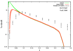
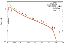
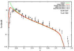
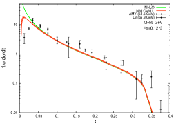
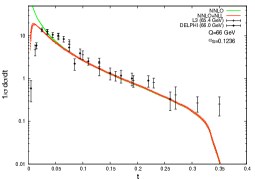
Figure 1: Fixed-order (NNLO), resummed (NNLO+NLL) and experimental thrust distributions: $Q=14-66$ GeV.

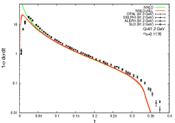
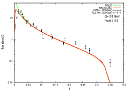
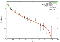
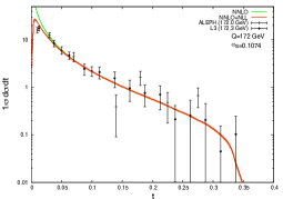
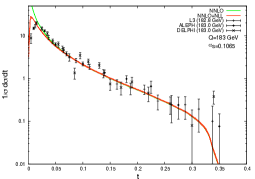
Figure 2: Fixed-order (NNLO), resummed (NNLO+NLL) and experimental thrust distributions: $Q=91-183$ GeV.

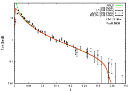
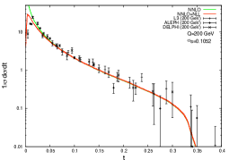
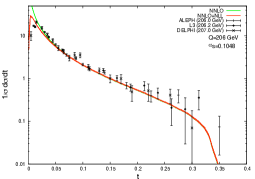
Figure 3: Fixed-order (NNLO), resummed (NNLO+NLL) and experimental thrust distributions: $Q=189-207$ GeV.

2.2 Resummation of large logarithms

The enhancement of the distribution at low $t$ due to soft or collinear gluon emission (as seen in Figs. 1- 3) is present at all orders in perturbation theory: the dominant term at $n$th order is typically of the form

$$\frac{1}{\sigma}\frac{d\sigma}{dt}\sim\alpha_{s}^{n}\frac{1}{t}\ln^{2n-1}\left(\frac{1}{t}\right).$$ (9)

Thus we see that at low $t$ the condition $\alpha_{s}\ll 1$ is not sufficient for a fixed-order prediction in perturbation theory to be accurate. Instead, we require $\alpha_{s}L^{2}\ll 1$, where $L\equiv\ln(1/t)$. To obtain accurate predictions in the two-jet limit $t\rightarrow 0$, we must therefore take account of these enhanced terms at all orders in perturbation theory by resumming them.

Resummation of large logarithms is possible for event shape variables $y$ that exponentiate four , i.e. their corresponding normalised cross section can be written in the form

$$R\left(y\right)=C\left(\alpha_{s}\right)\Sigma\left(y,\alpha_{s}\right)+D\left(y,\alpha_{s}\right),$$ (10)

where

$$C\left(\alpha_{s}\right) =1+\sum_{n=1}^{\infty}C_{n}\bar{\alpha}_{s}^{n},$$ (11)

$$\ln\Sigma\left(y,\alpha_{s}\right) =\sum_{n=1}^{\infty}\sum_{m=1}^{n+1}G_{nm}\bar{\alpha}_{s}^{n}L^{m}$$

$$=Lg_{1}\left(\alpha_{s}L\right)+g_{2}\left(\alpha_{s}L\right)+\alpha_{s}g_{3}\left(\alpha_{s}L\right)+\ldots,$$

$L=\ln(1/y)$ and $D\left(y,\alpha_{s}\right)$ is a remainder function that vanishes order-by-order in perturbation theory in the two-jet limit $y\rightarrow 0$. The functions $g_{i}\left(\alpha_{s}L\right)$ are power series in $\alpha_{s}L$ (with no leading constant term) and hence $Lg_{1}\left(\alpha_{s}L\right)$ sums all leading logarithms $\alpha_{s}^{n}L^{n+1}$, $g_{2}\left(\alpha_{s}L\right)$ sums all next-to-leading logarithms (NLL) $\alpha_{s}^{n}L^{n}$ and the subdominant logarithmic terms $\alpha_{s}^{n}L^{m}$ with $0<m<n$ are contained in the $g_{3},g_{4},\ldots$ terms. The functions $g_{i}$ thus resum the logarithmic contributions at all orders in perturbation theory, and knowledge of their form allows us to make accurate perturbative predictions in the range $\alpha_{s}L\lesssim 1$ – a significant improvement on the fixed-order range $\alpha_{s}L^{2}\ll 1$.

For thrust, the first two functions can be determined analytically by using the coherent branching formalism Dokshitzer:1982xr ; Bassetto:1984ik , which uses consecutive branchings from an initial quark-antiquark state to produce multi-parton final states to NLL accuracy. The results of this calculation depend upon the jet mass distribution $J\left(Q^{2},k^{2}\right)$ – the probability of producing a final state jet with invariant mass $k^{2}$ from a parent parton produced in a hard process at scale $Q^{2}$ – and its Laplace transform $\tilde{J}_{\nu}\left(Q^{2}\right)$. To the required accuracy, the thrust distribution is

$$\frac{1}{\sigma}\frac{d\sigma}{dt}=\frac{Q^{2}}{2\pi i}\int_{C}d\nu e^{t\nu Q^{2}}\left[\tilde{J}_{\nu}^{\mu}\left(Q^{2}\right)\right]^{2},$$ (12)

where the contour $C$ runs parallel to the imaginary axis on the right of all singularities of the integrand,

$$\ln\tilde{J}_{\nu}^{\mu}\left(Q^{2}\right) = \int_{0}^{1}\frac{du}{u}\left(e^{-u\nu Q^{2}}-1\right)\Biggl{[}\int_{u^{2}Q^{2}}^{uQ^{2}}\frac{d\mu^{2}}{\mu^{2}}C_{F}\frac{\alpha_{s}\left(\mu\right)}{\pi}$$ (13)

$$\left(1-K\frac{\alpha_{s}\left(\mu\right)}{2\pi}\right)^{-1}+\ldots\Biggr{]},$$

and

$$K=N\left(\frac{67}{18}-\frac{\pi^{2}}{6}\right)-\frac{5}{9}N_{F}\;.$$ (14)

This expression demonstrates explicitly that the divergence of $\alpha_{s}\left(\mu\right)$ at low $\mu$ will affect the perturbative thrust distribution – such effects are related to the renormalon mentioned earlier. To NLL accuracy, however, we can neglect the low $\mu$ region (although we will return to it in Sect. 4) to give the thrust resummation functions four

$$g_{1}\left(\alpha_{s}L\right)=2f_{1}\left(\beta_{0}\bar{\alpha}_{s}L\right),$$ (15)

$$g_{2}\left(\alpha_{s}L\right)=2f_{2}\left(\beta_{0}\bar{\alpha}_{s}L\right)-\ln\Gamma[1-2f_{1}\left(\beta_{0}\bar{\alpha}_{s}L\right)$$

$$\;\;\;\;-2\beta_{0}\bar{\alpha}_{s}Lf_{1}^{\prime}\left(\beta_{0}\bar{\alpha}_{s}L\right)],$$

where

$$f_{1}\left(x\right)= -\frac{C_{F}}{\beta_{0}x}[\left(1-2x\right)\ln\left(1-2x\right)$$ (16)

$$-2\left(1-x\right)\ln\left(1-x\right)],$$

$$f_{2}\left(x\right)= -\frac{C_{F}K}{\beta_{0}^{2}}\left[2\ln\left(1-x\right)-\ln\left(1-2x\right)\right]$$

$$-\frac{3C_{F}}{2\beta_{0}}\ln\left(1-x\right)-\frac{2C_{F}\gamma_{E}}{\beta_{0}}[\ln\left(1-x\right)$$

$$-\ln\left(1-2x\right)]-\frac{C_{F}\beta_{1}}{\beta_{0}^{3}}\bigl{[}\ln\left(1-2x\right)$$

$$-2\ln\left(1-x\right)+\frac{1}{2}\ln^{2}\left(1-2x\right)-\ln^{2}\left(1-x\right)\bigr{]},$$

with $\Gamma$ the Euler $\Gamma$-function, $\gamma_{E}$ the Euler constant, and $C_{F}$, $K$ and $\beta_{n}$ the constants previously defined.

By combining these with the fixed-order calculation, we can obtain a new estimate of the normalised cross section to NLL accuracy. This should particularly improve the fixed-order estimate in the two-jet region, where $L$ becomes large. Naively we would simply calculate $R\left(t\right)$ as defined in Eq. (10), but it turns out to be considerably simpler to consider $\ln R\left(t\right)$, as we recall next.

2.3 Log-R matching

In the log-R matching scheme, we rewrite the exponentiation formula as

$$\ln R\left(t\right)=F\left(\alpha_{s}\right)+\ln\Sigma\left(t,\alpha_{s}\right)+H\left(t,\alpha_{s}\right),$$ (17)

where $F\left(\alpha_{s}\right)$ is a power series in $\alpha_{s}$ and $H\left(t,\alpha_{s}\right)$ denotes the remainder function which vanishes as $t\rightarrow 0$.

For a fixed-order perturbative calculation of $R\left(t\right)$ to order $M$, we can write Eq. (6) as

$$\ln R\left(t\right) =\ln\left(1+\sum_{n=1}^{M}\bar{\alpha}_{s}^{n}R_{n}\left(t\right)\right)$$ (18)

$$=\sum_{n=1}^{M}\bar{\alpha}_{s}^{n}R_{n}\left(t\right)-\frac{1}{2}\left(\sum_{n=1}^{M}\bar{\alpha}_{s}^{n}R_{n}\left(t\right)\right)^{2}$$

$$+\frac{1}{3}\left(\sum_{n=1}^{M}\bar{\alpha}_{s}^{n}R_{n}\left(t\right)\right)^{3}-\ldots.$$

The matched estimate is obtained by combining the $M$th order perturbative result with the resummed contributions and subtracting the terms of order $\leq M$ in $\ln\Sigma$ (as these are already accounted for in the fixed-order terms). Thus for a fixed-order calculation to order $\alpha_{s}^{3}$, the matched estimate after resumming large logarithms to NLL accuracy is

$$\ln R\left(t\right) =Lg_{1}\left(\alpha_{s}L\right)+g_{2}\left(\alpha_{s}L\right)$$ (19)

$$+\bar{\alpha}_{s}\left(R_{1}\left(t\right)-G_{11}L-G_{12}L^{2}\right)$$

$$+\bar{\alpha}_{s}^{2}\left(R_{2}\left(t\right)-\frac{1}{2}\left[R_{1}\left(t\right)\right]^{2}-G_{22}L^{2}-G_{23}L^{3}\right)$$

$$+\bar{\alpha}_{s}^{3}\biggl{(}R_{3}\left(t\right)-R_{1}\left(t\right)R_{2}\left(t\right)+\frac{1}{3}\left[R_{1}\left(t\right)\right]^{3}$$

$$-G_{33}L^{3}-G_{34}L^{4}\biggr{)}.$$

The coefficients $G_{nm}$ can be extracted by expanding the functions $g_{1}\left(\alpha_{s}L\right)$ and $g_{2}\left(\alpha_{s}L\right)$ as power series in $\alpha_{s}L$ and comparing them with the definition (11) of $G_{nm}$:

$$G_{11} =3C_{F},$$ (20)

$$G_{12} =-2C_{F},$$

$$G_{22} =-\frac{C_{F}}{36}\left[48\pi^{2}C_{F}+\left(169-12\pi^{2}\right)N-22N_{F}\right],$$

$$G_{23} =-\frac{C_{F}}{3}\left(11N-2N_{F}\right),$$

$$G_{33} =\frac{C_{F}}{108}\bigl{[}2304\zeta\left(3\right)C_{F}^{2}-792\pi^{2}NC_{F}$$

$$-\left(3197-132\pi^{2}\right)N^{2}+\left(108+144\pi^{2}\right)C_{F}N_{F}$$

$$+\left(1024-24\pi^{2}\right)NN_{F}-68N_{F}^{2}\bigr{]},$$

$$G_{34} =-\frac{7}{108}C_{F}\left(11N-2N_{F}\right)^{2},$$

where $\zeta\left(3\right)=1.202057\ldots$.

There are two reasons why it is simpler to use this log-$R$ matching scheme rather than $R$ matching (i.e. evaluating Eq. (10) explicitly to NLL precision). Firstly, we do not have to be concerned with the $C\left(\alpha_{s}\right)$ and $D\left(t,\alpha_{s}\right)$ terms in (10), for which we do not have analytic expressions but which contribute to the fixed-order calculation – these are contained in $R_{1}\left(t\right)$, $R_{2}\left(t\right)$, etc. Secondly, it is easier to impose physical boundary conditions on the normalised cross section, namely

$$R\left(t=t_{max}\right)=1,$$ (21)

by definition of the normalised cross section, and

$$\frac{dR}{dt}\left(t=t_{max}\right)=0,$$ (22)

as there is an upper kinematic limit $t_{\text{max}}$ on the thrust for a given number of final-state partons. Although the resummed logarithmic terms are small at high $t$, $dR/dt$ is also small and so these terms can cause relatively large unphysical effects if we do not impose these conditions.

The above constraints are automatically obeyed by the fixed-order terms $R_{n}\left(t\right)$ but not by the resummed terms, as we have neglected the subdominant logarithms $g_{3}\left(\alpha_{s}L\right)$, $g_{4}\left(\alpha_{s}L\right)$ etc. To satisfy these constraints, we therefore require

$$Q\left(t\right) =Lg_{1}\left(\alpha_{s}L\right)+g_{2}\left(\alpha_{s}L\right)-\bar{\alpha}_{s}\left(G_{11}L+G_{12}L^{2}\right)$$ (23)

$$-\bar{\alpha}_{s}^{2}\left(G_{22}L^{2}+G_{23}L^{3}\right)-\bar{\alpha}_{s}^{3}\left(G_{33}L^{3}+G_{34}L^{4}\right)$$

and its first derivative to vanish at $t=t_{max}$. $Q\left(t\right)$ corresponds to the resummed logarithmic terms of order $L^{4}$ and higher and hence at small $L$,

$$t\frac{dQ}{dt}=aL^{3}+bL^{4}+cL^{5}+\ldots.$$ (24)

By making the replacement

$$L\rightarrow\tilde{L}=\ln\left(1+\frac{1}{t}-\frac{1}{t_{max}}\right),$$ (25)

the boundary conditions are satisfied as $\tilde{L}\left(t_{max}\right)=0$. This does introduce corrections to the expression for $\ln R\left(t\right)$ but these are power-suppressed at small $t$:

$$\tilde{L}\left(t\right) =\ln\left(\frac{1}{t}\right)+\ln\left(1-\frac{t}{t_{max}}+t\right)$$ (26)

$$=L\left(t\right)+\left(t-\frac{t}{t_{max}}\right)-\frac{1}{2}\left(t-\frac{t}{t_{max}}\right)^{2}+\ldots,$$

and so $\tilde{L}\left(t\right)\rightarrow L\left(t\right)$ in the important limit $t\rightarrow 0$.

3 Results of NNLO+NLL matching

To perform the matching, the integrated perturbation series coefficients are required as in Eq. (19). For $R_{1}\left(t\right)$, the analytic result is

$$R_{1}\left(t\right)= -\frac{8}{3}\ln^{2}\left(\frac{t}{1-t}\right)-4\left(1-2t\right)\ln\left(\frac{t}{1-2t}\right)+\frac{4\pi^{2}}{9}$$ (27)

$$-\frac{10}{3}+8t+6t^{2}-\frac{16}{3}\text{Li}_{2}\left(\frac{t}{1-t}\right),$$

where

$$\text{Li}_{2}\left(z\right)\equiv\int^{0}_{z}dx\frac{\ln\left(1-x\right)}{x}$$ (28)

is the dilogarithm function. $R_{2}\left(t\right)$ and $R_{3}\left(t\right)$ were obtained by interpolating the differential results from EERAD3 and then numerically integrating them. For $R_{3}\left(t\right)$, the EERAD3 results were first smoothed by taking

$$\frac{dR_{3}}{dt}\left(t_{i}\right)\rightarrow\frac{1}{3}\left[\frac{dR_{3}}{dt}\left(t_{i+1}\right)+\frac{dR_{3}}{dt}\left(t_{i}\right)+\frac{dR_{3}}{dt}\left(t_{i-1}\right)\right],$$ (29)

repeatedly until a smooth curve was obtained. The peak near $t=0$ had to be reintroduced by hand, as this smoothing technique always results in the peak value being reduced.

$R\left(t\right)$ was computed to NNLO+NLL precision using Eqs. (19) and (26) with $t_{max}=0.42$ in $\tilde{L}$, as this is the maximum value of $t$ kinematically allowed in the five parton limit. The differential cross section was then obtained by numerically differentiating $R(t)$. The results at a range of energies are shown by the red/darker curves in Figs 1-3. The values of $\alpha_{s}\left(Q\right)$ were calculated as described earlier for the unresummed NNLO (green/lighter) curves. The shaded area around each line shows the renormalisation scale uncertainty found by taking $\mu_{R}^{2}\in\left[Q^{2}/2,2Q^{2}\right]$.

3.1 Comparison with experimental data

The matched, resummed differential thrust distribution was compared with data from a wide range of experiments, as listed in Table 1. The points in Figs. 1-3 show the data at an illustrative selection of energies. The error bars represent the experimental statistical and systematic errors, added in quadrature.

Experiment	$Q$/GeV	Ref.	No. Pts.	$\chi^{2}$
TASSO	$14.0$	tasso	4	8.2
TASSO	$22.0$	tasso	6	2.8
TASSO	$35.0$	tasso	8	0.7
JADE	$35.0$	jade	10	10.5
L3	$41.4$	l3	8	3.4
JADE	$44.0$	jade	10	3.8
TASSO	$44.0$	tasso	8	6.8
DELPHI	$45.0$	delphi	11	11.6
AMY	$54.5$	amy	4	4.9
L3	$55.3$	l3	8	3.2
L3	$65.4$	l3	8	7.5
DELPHI	$66.0$	delphi	11	14.5
L3	$75.7$	l3	8	1.9
DELPHI	$76.0$	delphi	11	10.3
L3	$82.3$	l3	8	4.0
L3	$85.1$	l3	8	3.6
OPAL	$91.0$	opal	5	11.9
ALEPH	$91.2$	aleph	27	16.1
DELPHI	$91.2$	delphi	11	18.8
SLD	$91.2$	sld	6	2.7
L3	$130.1$	l3	10	14.6
ALEPH	$133.0$	aleph	6	7.2
OPAL	$133.0$	opal	5	6.5
L3	$136.1$	l3	10	37.3
ALEPH	$161.0$	aleph	6	5.5
L3	$161.3$	l3	10	4.0
ALEPH	$172.0$	aleph	6	14.0
L3	$172.3$	l3	10	2.1
OPAL	$177.0$	opal	5	1.1
L3	$182.8$	l3	10	2.7
ALEPH	$183.0$	aleph	6	4.0
DELPHI	$183.0$	delphi	13	33.1
L3	$188.6$	l3	10	3.4
ALEPH	$189.0$	aleph	6	6.7
DELPHI	$189.0$	delphi	13	22.7
DELPHI	$192.0$	delphi	13	12.1
L3	$194.4$	l3	10	1.2
DELPHI	$196.0$	delphi	13	39.7
OPAL	$197.0$	opal	5	10.0
ALEPH	$200.0$	aleph	6	21.0
DELPHI	$200.0$	delphi	13	7.1
L3	$200.0$	l3	9	6.5
DELPHI	$202.0$	delphi	13	14.9
DELPHI	$205.0$	delphi	13	12.6
ALEPH	$206.0$	aleph	6	7.0
L3	$206.2$	l3	10	10.0
DELPHI	$207.0$	delphi	13	11.7
Total			430	466.0

Table 1: Data sets used and best-fit $\chi^{2}$ contributions.

There are a few features common to the graphs at all energies. Firstly, the resummed distribution and the NNLO distribution are almost identical away from the two-jet region. However, in this low-$t$ limit the resummed distribution peaks, in line with the experimental data, whereas the NNLO distribution carries on increasing. Thus resummation has significantly improved the theoretical prediction in the two-jet limit, as we had expected.

It should be noted that the kink around $t=0.33$ in all of the curves is due to the LO term vanishing here for kinematic reasons. One would expect that with many higher-order perturbation theory terms taken into account (i.e. more partons present in the final state), this would gradually smoothen, in line with the experimental data.

At all energies, the overall shape of the theoretical distribution is similar to that of the data, but is shifted to a lower value of $t$. This apparent shift $\delta t$ has a clear energy dependence – at the upper end of the energy range considered here, the NNLO+NLL and experimental distributions are fairly close and the shift $\delta t$ is a very small correction. On decreasing the energy, the shift becomes more pronounced and at low energies the theoretical distribution is clearly not consistent with the data. There is no obvious way that this could be remedied by the inclusion of sub-leading logarithms or higher fixed-order terms, and so we now turn to considering non-perturbative effects for an explanation. The increasing discrepancy at low energies is also consistent with this interpretation, as we expect such effects to have a $1/Q$ dependence, as mentioned in Sect. 1. To verify that these discrepancies are due to non-perturbative effects, the exact form of their energy dependence was investigated.

3.2 Power dependence of discrepancies

As both the experimental data and EERAD3 results are given as histograms, and not in terms of individual values of $t$, the integrated thrust distribution $R\left(t\right)$ should be slightly more accurate than $d\sigma/dt$ as it does not involve the assumption of a uniform distribution over the width of each histogram bin $\Delta t$.

Graphs of $\ln\left(R_{\text{theory}}-R_{\text{expt}}\right)$ against $\ln\left(Q/\text{GeV}\right)$ were plotted for $0.025\leq t\leq 0.24$ and, anticipating corrections proportional to an inverse power of $Q$, a linear fit was made to each plot such that the gradient $n$ of the straight line gives the power dependence of the required correction ($\propto Q^{n}$). The results are shown in Figs. 4-6. This $t$ range was chosen since at lower values of $t$ there is no obvious straight line (due to the distributions peaking), and at higher values of $t$ the percentage errors on the gradient become large due to $R_{\text{theory}}-R_{\text{expt}}$ quickly decreasing to zero (as both normalised cross-sections converge to 1).

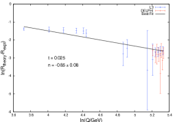
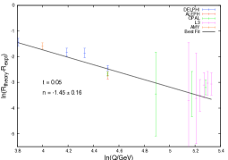
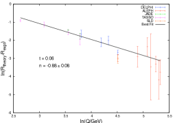
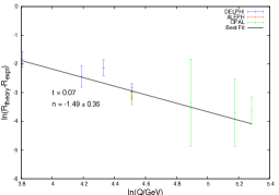
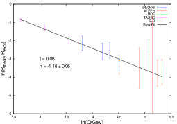
Figure 4: Power dependence of corrections required to resolve theory/data discrepancy: $t=0.025-0.08$.

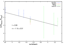
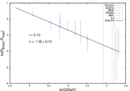
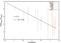
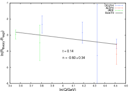
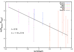
Figure 5: Power dependence of corrections required to resolve theory/data discrepancy: $t=0.09-0.16$.

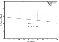
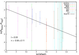
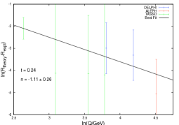
Figure 6: Power dependence of corrections required to resolve theory/data discrepancy: $t=0.18-0.24$.

Although not totally conclusive, these results are consistent with power corrections of the form $1/Q$, and we turn now to considering the quantitative form of these non-perturbative corrections to the thrust distribution.

4 Non-perturbative corrections

4.1 The low-scale effective coupling

Although there are various ways to phenomenologically treat non-perturbative effects in QCD, one of the most intuitive is by means of a low-scale effective coupling one . In this approach, the running coupling (7) is replaced by an effective coupling $\alpha_{\text{eff}}\left(\mu\right)$, which differs from the standard perturbative $\alpha_{s}(\mu)$ in the infra-red region where the latter diverges. Using this finite effective coupling allows us to use the formalism of perturbation theory to describe non-perturbative effects which cannot be probed using standard perturbative QCD.

Various forms for $\alpha_{\text{eff}}(\mu)$ have been proposed Solovtsov:1997at ; nine that have high-energy behaviour consistent with $\alpha_{s}$, but we will not be concerned with their details here. The only parameter we require is the ‘average’ value of the effective coupling below the infra-red matching scale $\mu_{I}$ where $\alpha_{s}$ and $\alpha_{\text{{eff}}}$ begin to differ:

$$\alpha_{0}\left(\mu_{I}\right)\equiv\frac{1}{\mu_{I}}\int_{0}^{\mu_{I}}d\mu\text{ }\alpha_{\text{eff}}\left(\mu\right).$$ (30)

We make the additional assumption that $\alpha_{\text{eff}}$ is small enough in the infra-red region that we can neglect terms of order $\alpha_{\text{eff}}^{2}$ and higher.

4.2 Non-perturbative shift in thrust distribution

In deriving the form of the NNLO+NLL prediction used earlier, the low $\mu$ region in Eq. (13) was neglected as it produced a subleading contribution. We now include this region by subtracting the fixed-order NNLO contribution from $\mu\leq\mu_{I}$ and replacing it with a contribution due to the effective coupling. We are thus removing the renormalon contributions to the perturbation series (up to NNLO) and incorporating all $1/Q$-dependent behaviour into $\alpha_{\text{eff}}$.

Firstly, we note that the order of integration in (13) can be changed, to give

$$\ln\tilde{J}_{\nu}^{\mu}\left(Q^{2}\right) = \frac{2C_{F}}{\pi}\int_{0}^{Q}\frac{d\mu}{\mu}\alpha_{s}\left(\mu\right)\left(1-K\frac{\alpha_{s}\left(\mu\right)}{2\pi}\right)^{-1}$$ (31)

$$\int_{\frac{\mu^{2}}{Q^{2}}}^{\frac{\mu}{Q}}\frac{du}{u}\left(e^{-u\nu Q^{2}}-1\right)\;.$$

Inserting the NNLO perturbative running coupling

$$\alpha_{s}\left(\mu\right) = \alpha_{s}\left(\mu_{R}\right)+\alpha_{s}^{2}\left(\mu_{R}\right)\frac{\beta_{0}}{\pi}\ln\frac{\mu_{R}}{\mu}$$ (32)

$$+ \alpha_{s}^{3}\left(\mu_{R}\right)\left[\left(\frac{\beta_{0}}{\pi}\right)^{2}\ln^{2}\frac{\mu_{R}}{\mu}+\frac{\beta_{1}}{2\pi^{2}}\ln\frac{\mu_{R}}{\mu}\right],$$

expanding the exponential to first order and integrating over the range $0\leq\mu\leq\mu_{I}$ gives an NNLO contribution of

$$-\frac{2C_{F}}{\pi}\frac{\mu_{I}}{Q}\Biggl{\{}\alpha_{s}\left(\mu_{R}\right)+\alpha_{s}^{2}\left(\mu_{R}\right)\frac{\beta_{0}}{\pi}\left(\ln\frac{\mu_{R}}{\mu_{I}}+\frac{K}{2\beta_{0}}+1\right)$$ (33)

$$+\alpha_{s}^{3}\left(\mu_{R}\right)\left(\frac{\beta_{0}}{\pi}\right)^{2}\biggl{[}\ln^{2}\frac{\mu_{R}}{\mu_{I}}+\left(\ln\frac{\mu_{R}}{\mu_{I}}+1\right)$$

$$\left(2+\frac{\beta_{1}}{2\beta_{0}^{2}}+\frac{K}{\beta_{0}}\right)+\frac{K^{2}}{4\beta_{0}^{2}}\biggr{]}\Biggr{\}}\nu Q^{2}.$$

It should be noted that $t$ is the conjugate variable to $\nu Q^{2}$ in the Laplace transform (12) and thus the first-order expansion of the exponential will only be a valid approximation in the limit $t\gg\mu_{I}/Q$. Below this, we would need to retain higher order terms in the expansion, which would require us to have a specific form for $\alpha_{\text{eff}}\left(\mu\right)$.

Following a similar procedure with $\alpha_{\text{eff}}\left(\mu\right)$ in the place of $\alpha_{s}\left(\mu\right)$ gives a non-perturbative contribution of

$$-\frac{2C_{F}}{\pi}\int_{0}^{\mu_{I}}d\mu\text{ }\alpha_{\text{eff}}\left(\mu\right)\nu Q\equiv-\frac{2C_{F}}{\pi}\frac{\mu_{I}}{Q}\alpha_{0}\left(\mu_{I}\right)\nu Q^{2},$$ (34)

where we have neglected terms of order $\alpha^{2}_{\text{eff}}$ as previously noted.

By adding this, after subtracting the perturbative contribution (33), we obtain the change in the quark jet mass distribution caused by changing from a perturbative to an effective coupling in the low-scale region below $\mu_{I}$.

Substituting the result into Eq. (12), we see that the effect of this non-perturbative contribution is to shift the thrust distribution by an amount $\delta t$, such that

$$\left.\frac{1}{\sigma}\frac{d\sigma}{dt}\right|_{t}=\left.\left(\frac{1}{\sigma}\frac{d\sigma}{dt}\right)^{\text{pert.}}\right|_{t+\delta t},$$ (35)

where

$$\delta t= -\frac{4C_{F}}{\pi}\frac{\mu_{I}}{Q}\Biggl{\{}\alpha_{0}\left(\mu_{I}\right)-\alpha_{s}\left(\mu_{R}\right)$$ (36)

$$-\alpha_{s}^{2}\left(\mu_{R}\right)\frac{\beta_{0}}{\pi}\left(\ln\frac{\mu_{R}}{\mu_{I}}+\frac{K}{2\beta_{0}}+1\right)$$

$$-\alpha_{s}^{3}\left(\mu_{R}\right)\left(\frac{\beta_{0}}{\pi}\right)^{2}\biggl{[}\ln^{2}\frac{\mu_{R}}{\mu_{I}}+\left(\ln\frac{\mu_{R}}{\mu_{I}}+1\right)$$

$$\left(2+\frac{\beta_{1}}{2\beta_{0}^{2}}+\frac{K}{\beta_{0}}\right)+\frac{K^{2}}{4\beta_{0}^{2}}\biggr{]}\Biggr{\}},$$

to NNLO. This $1/Q$-dependent shift is precisely what is required to account for the differences between the perturbative and experimental distributions seen in Sect. 3.

4.3 Determination of $\alpha_{s}$ and $\alpha_{0}$

By applying the shift (36) to the perturbative results, we expect to reduce significantly the differences between the theoretical and experimental distributions. Comparison of these differences to the predicted form of $\delta t$ allows us to estimate the values of $\alpha_{0}$ and $\alpha_{s}$.

Maximum accuracy was obtained by comparing the experimental distribution with a discretely-defined theoretical distribution

$$\frac{R\left(t+\Delta t\right)-R\left(t\right)}{\Delta t},$$ (37)

where $\Delta t$ is the bin width of the experimental data.

The NNLO+NLL+shift distribution was calculated as a function of $\alpha_{0}$ and $\Lambda_{\overline{MS}}^{\left(5\right)}$. This calculation was performed for $0.05\leq t\leq 0.33$, at the centre-of-mass energies listed previously in Table 1 (i.e. in the range $14$ GeV$\leq Q\leq 207$ GeV). $\chi^{2}$ was calculated for each pair of input parameters, with its minimum corresponding to the best-fit values.

The upper limit for the fits was chosen as $t=0.33$ since the difference between the theoretical and experimental distributions above this value is largely due to the small number of final state partons in the theoretical calculation, as previously explained, rather than to any non-perturbative effects. We noted previously that the non-perturbative results are strictly valid only in the range $t\gg\mu_{I}/Q$; in fact we found satisfactory fits using an energy-dependent lower cut-off $t\geq\max\{\mu_{I}/Q,0.05\}$.

For infra-red matching scale $\mu_{I}=2$ GeV, best fit values of

$$\alpha_{0}\left(2\text{ GeV}\right) =0.59\pm 0.03\;,$$ (38)

$$\Lambda_{\overline{MS}}^{\left(5\right)} =0.190^{+0.025}_{-0.022}\text{ GeV}$$

were obtained, with $\chi^{2}/\text{d.o.f.}=466.0/428\approx 1.09$. The quoted errors correspond to one standard deviation, computed as recommended by the Particle Data Group Amsler:2008zz : the value of $\chi^{2}$ corresponding to the $1\sigma$ (68.3% C.L.) contour was rescaled by the value of $\chi^{2}/\text{d.o.f.}$, giving $\chi^{2}=480.6$, i.e. $\Delta\chi^{2}=14.6$.

The contribution to $\chi^{2}$ from each data set is shown in Table 1. It should be noted that the few data sets with $\chi^{2}/\text{no. pts.}\gg 1$ are not generally inconsistent with the shifted distribution, but simply have a few outlying points giving a large contribution.

The contour plot in Fig. 7 shows the ranges of $\alpha_{0}$ and $\Lambda_{\overline{MS}}^{\left(5\right)}$ which give fits within $\Delta\chi^{2}$ of the best-fit value of $\chi^{2}$, and also demonstrates the correlation between these two parameters.

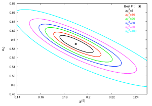
Figure 7: $\chi^{2}$ contour plot in $\left(\Lambda_{\overline{MS}}^{\left(5\right)}\text{ , }\alpha_{0}\right)$ space.

Varying the renormalisation scale $\mu_{R}^{2}\in\left[Q^{2}/2,2Q^{2}\right]$ gave best fit values in the range $\alpha_{0}\left(2\text{ GeV}\right)=0.585$, $\Lambda_{\overline{MS}}^{\left(5\right)}=0.173$ GeV to $\alpha_{0}\left(2\text{ GeV}\right)=0.598$, $\Lambda_{\overline{MS}}^{\left(5\right)}=0.210$ GeV with no significant change in the quality of fit. Thus we find

$$\Lambda_{\overline{MS}}^{\left(5\right)}=0.190^{+0.025+0.020}_{-0.022-0.017}\text{ GeV}$$ (39)

where the first error is the combined experimental statistical and systematic error and the second is due to the theoretical renormalisation scale uncertainty. The corresponding strong coupling constant is

$$\alpha_{s}\left(91.2\text{ GeV}\right)=0.1164^{+0.0022+0.0017}_{-0.0021-0.0016}\;,$$ (40)

or, combining all the errors in quadrature,

$$\alpha_{s}\left(91.2\text{ GeV}\right)=0.1164^{+0.0028}_{-0.0026}\;,$$ (41)

in good agreement with the world average value of 0.1176 Amsler:2008zz .

To assess the importance of the NNLO terms, the analysis was repeated with all those terms omitted, i.e.  combining NLO+NLL in perturbation theory with Eq. (36) without the ${\cal O}(\alpha_{s}^{3})$ contribution. The resulting best fit values were

$$\alpha_{0}\left(2\text{ GeV}\right) =0.51\pm 0.04\;,$$ (42)

$$\Lambda_{\overline{MS}}^{\left(5\right)} =0.214^{+0.032+0.034}_{-0.027-0.026}\text{ GeV}\;,$$

$$\alpha_{s}\left(91.2\text{ GeV}\right) =0.1185^{+0.0025+0.0027}_{-0.0024-0.0023}$$

with $\chi^{2}/\text{d.o.f.}=515.1/428\approx 1.20$. Thus the NLO and NNLO results are consistent but the inclusion of NNLO terms consistently in both the perturbative prediction and the power correction improves the quality of the fit and reduces the errors.

The most complete previous NLO study along similar lines MovillaFernandez:2001ed , combining NLO+NLL in perturbation theory with the NLO equivalent of Eq. (36) and covering a variety of event shapes but a slightly narrower range of energies than that used here, obtained the overall best fit at

$$\alpha_{s}\left(91.2\text{ GeV}\right) =0.1171^{+0.0032}_{-0.0020},$$ (43)

$$\alpha_{0}\left(2\text{ GeV}\right) =0.513^{+0.066}_{-0.045}$$

in good agreement with our results. Their fit to the thrust distribution alone gave

$$\alpha_{s}\left(91.2\text{ GeV}\right) =0.1173^{+0.0063}_{-0.0051},$$ (44)

$$\alpha_{0}\left(2\text{ GeV}\right) =0.492^{+0.084}_{-0.070}$$

also in good agreement.

In the recent NNLO analysis eleven , a range of event shapes at energies at and above 91.2 GeV were fitted without resummation; non-perturbative effects were estimated using Monte Carlo event generators. The value obtained for the strong coupling was $\alpha_{s}\left(91.2\text{ GeV}\right)=0.1240\pm 0.0033$.

To estimate the dependence of our results upon the infra-red matching scale, a fit with $\mu_{I}=3$ GeV was made, yielding $\alpha_{0}\left(3\text{ GeV}\right)=0.458\pm 0.025$ and $\Lambda_{\overline{MS}}^{\left(5\right)}=0.202^{+0.034}_{-0.027}$, with $\chi^{2}/\text{d.o.f.}\approx 1.09$. Thus the fit remains good and the value obtained for $\Lambda_{\overline{MS}}^{\left(5\right)}$ is stable under variation of $\mu_{I}$, while the value of $\alpha_{0}$ decreases as expected for a running effective coupling. Indeed, the implied mean value of $\alpha_{\text{eff}}$ in the range 2-3 GeV,

$$\overline{\alpha}_{\text{eff}}=3\,\alpha_{0}\left(3\text{ GeV}\right)-2\,\alpha_{0}\left(2\text{ GeV}\right)=0.19\pm 0.10$$ (45)

is consistent with the perturbative value $\alpha_{s}\left(2.5\text{ GeV}\right)=0.26$.

4.4 Final comparison with experimental distributions

Figures 8-10 show the final (NNLO+NLL+shift) theoretical distributions in comparison to the experimental ones, with the best-fit values of $\alpha_{0}$ and $\alpha_{s}$ assumed. The shaded area around the unshifted distribution is the renormalisation scale uncertainty found by varying $\mu_{R}^{2}\in\left[Q^{2}/2,2Q^{2}\right]$, and the shaded area around the shifted distribution is the corresponding error found by varying between the best fit limits obtained previously ($\alpha_{0}\left(2\text{ GeV}\right)=0.585$, $\Lambda_{\overline{MS}}^{\left(5\right)}=0.173$ GeV and $\alpha_{0}\left(2\text{ GeV}\right)=0.598$, $\Lambda_{\overline{MS}}^{\left(5\right)}=0.210$ GeV).

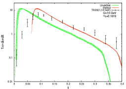
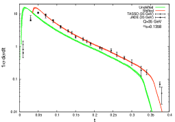
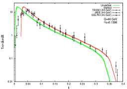
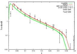
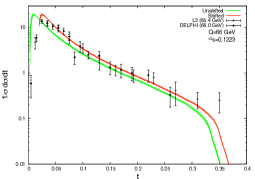
Figure 8: Comparison of shifted, unshifted and experimental thrust distributions: $Q=14-66$ GeV.

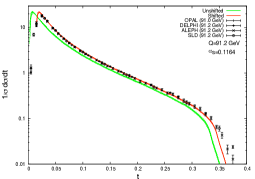
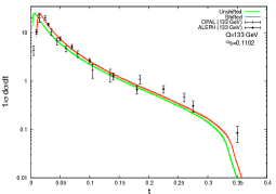
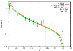
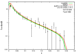
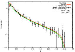
Figure 9: Comparison of shifted, unshifted and experimental thrust distributions: $Q=91-183$ GeV.

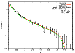
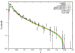
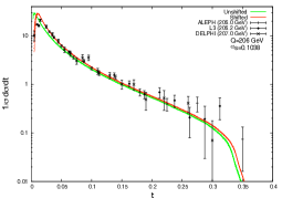
Figure 10: Comparison of shifted, unshifted and experimental thrust distributions: $Q=189-207$ GeV.

It is clearly seen that inclusion of the shift results in a significantly more accurate distribution over the fit range, particularly for the lower energies. As the best fit value of $\alpha_{s}$ is very close to the world average, the unshifted distributions here are essentially the same as those in Figs. 1-3.

5 Conclusions

We have seen that the extension of the NNLO perturbative distribution to NNLO+NLL accuracy results in an improved matching with experiment, particularly in the low $t$ region.

Analysis of the difference between the perturbative and experimental distributions over a range of energies showed that $1/Q$ power corrections were required to account for this difference. Replacement of the perturbative strong coupling with an effective coupling below an infra-red matching scale was used to include such non-perturbative corrections in our theoretical calculation and resulted in a $1/Q$-dependent shift in the distribution. With best-fit values $\alpha_{0}\left(2\text{ GeV}\right)=0.59\pm 0.03$ and $\alpha_{s}\left(91.2\text{ GeV}\right)=0.1164^{+0.0028}_{-0.0026}$, this gave a significantly improved matching with the experimental distributions in the range $14\text{ GeV}\leq Q\leq 207\text{ GeV}$. These values are consistent with those achieved in similar analyses to NLO, as well as with the world-average value of $\alpha_{s}$.

The agreement of the $\alpha_{0}$ and $\alpha_{s}$ values from the analysis at NNLO+NLL with those obtained at NLO+NLL is a non-trivial test of the low-scale effective coupling hypothesis. The presence of the ${\cal O}(\alpha_{s}^{3})$ term in Eq. (36), which amounts to about 80% of the ${\cal O}(\alpha_{s}^{2})$ term, means that we are not simply adding a $1/Q$ correction to the perturbative result, but rather that we are regularizing the divergent renormalon contribution by modifying the strong coupling at low scales. This implies that the explicit non-perturbative $1/Q$ shift applied to the perturbative prediction becomes smaller as higher orders are computed, and would eventually change sign at sufficiently high orders, as the renormalon contribution grows indefinitely.

A similar analysis to that in this work could be repeated for other event shape variables whose distributions have been determined perturbatively to NNLO and for which resummation of large logarithms is possible. Perturbative resummed calculations of such distributions have been performed twelve but non-perturbative effects have not been included in the way advocated here – they are not necessarily simple shifts as in the case of thrust. It would also be of interest to combine the present approach to non-perturbative effects with soft-collinear effective theory, which permits the resummation of next-to-next-to-leading logarithms Becher:2008cf .

References

- (1) Y. L. Dokshitzer and B. R. Webber, Phys. Lett. B 404 (1997) 321 [arXiv:hep-ph/9704298].
- (2) M. Beneke, Phys. Rept. 317 (1999) 1 [arXiv:hep-ph/9807443].
- (3) M. Beneke and V. M. Braun, arXiv:hep-ph/0010208.
- (4) Y. L. Dokshitzer, G. Marchesini and B. R. Webber, Nucl. Phys. B 469 (1996) 93 [arXiv:hep-ph/9512336].
- (5) A. Gehrmann-De Ridder, T. Gehrmann, E. W. N. Glover and G. Heinrich, Phys. Rev. Lett. 99 (2007) 132002 [arXiv:0707.1285 [hep-ph]].
- (6) A. Gehrmann-De Ridder, T. Gehrmann, E. W. N. Glover and G. Heinrich, JHEP 0712 (2007) 094 [arXiv:0711.4711 [hep-ph]].
- (7) A. Gehrmann-De Ridder, T. Gehrmann, E. W. N. Glover and G. Heinrich, JHEP 0711 (2007) 058 [arXiv:0710.0346 [hep-ph]].
- (8) S. Weinzierl, arXiv:0807.3241 [hep-ph].
- (9) C. Amsler et al. [Particle Data Group], Phys. Lett. B 667 (2008) 1.
- (10) S. Catani, L. Trentadue, G. Turnock and B. R. Webber, Nucl. Phys. B 407 (1993) 03.
- (11) Y. L. Dokshitzer, V. S. Fadin and V. A. Khoze, Z. Phys. C 15 (1982) 325; Z. Phys. C 18 (1983) 37.
- (12) A. Bassetto, M. Ciafaloni and G. Marchesini, Phys. Rept. 100, 201 (1983).
- (13) S. Catani, B. R. Webber and G. Marchesini, Nucl. Phys. B 349 (1991) 635.
- (14) TASSO Collaboration (W. Braunschweig et al.), Z. Phys. C 47 (1990) 187.
- (15) JADE Collaboration (P .A. Movilla Fernandez et al.), Eur. Phys. J. C 1 (1998) 461 [arXiv:hep-ex/9708034].
- (16) L3 Collaboration (P. Achard et al.), Phys. Rept. 399 (2004) 71 [arXiv:hep-ex/0406049].
- (17) DELPHI Collaboration (J. Abdallah et al.), Eur. Phys. J. C 29 (2003) 285 [arXiv:hep-ex/0307048].
- (18) AMY Collaboration (Y. K. Li et al.), Phys. Rev. D 41 (1990) 2675.
- (19) OPAL Collaboration (G. Abbiendi et al.), Eur. Phys. J. C 40 (2005) 287 [arXiv:hep-ex/0503051].
- (20) ALEPH Collaboration (A. Heister et al.), Eur. Phys. J. C 35 (2004) 457.
- (21) SLD Collaboration (K. Abe et al.), Phys. Rev. D 51 (1995) 962 [arXiv:hep-ex/9501003].
- (22) I. L. Solovtsov and D. V. Shirkov, Phys. Lett. B 442 (1998) 344 [arXiv:hep-ph/9711251]; Theor. Math. Phys. 150 (2007) 132 [arXiv:hep-ph/0611229].
- (23) B. R. Webber, JHEP 9810 (1998) 012 [arXiv:hep-ph/9805484].
- (24) P. A. Movilla Fernandez, S. Bethke, O. Biebel and S. Kluth, Eur. Phys. J. C 22 (2001) 1 [arXiv:hep-ex/0105059].
- (25) G. Dissertori, A. Gehrmann-De Ridder, T. Gehrmann, E. W. N. Glover, G. Heinrich and H. Stenzel, JHEP 0802 (2008) 040 [arXiv:0712.0327 [hep-ph]].
- (26) T. Gehrmann, G. Luisoni and H. Stenzel, Phys. Lett. B 664 (2008) 265 [arXiv:0803.0695 [hep-ph]].
- (27) T. Becher and M. D. Schwartz, JHEP 0807 (2008) 034 [arXiv:0803.0342 [hep-ph]].