The velocity–density relation in the spherical model

Abstract

We study the cosmic velocity–density relation using the spherical collapse model (SCM) as a proxy to non-linear dynamics. Although the dependence of this relation on cosmological parameters is known to be weak, we retain the density parameter $\Omega_{\rm m}$ in SCM equations, in order to study the limit $\Omega_{\rm m}\to 0$. We show that in this regime the considered relation is strictly linear, for arbitrary values of the density contrast, on the contrary to some claims in the literature. On the other hand, we confirm that for realistic values of $\Omega_{\rm m}$ the exact relation in the SCM is well approximated by the classic formula of Bernardeau (1992), both for voids ($\delta<0$) and for overdensities up to $\delta\sim 2$ – $3$. Inspired by this fact, we find further analytic approximations to the relation for the whole range $\delta\in[-1,\infty)$. Our formula for voids accounts for the weak $\Omega_{\rm m}$-dependence of their maximal rate of expansion, which for $\Omega_{\rm m}<1$ is slightly smaller that $3/2$. For positive density contrasts, we find a simple relation

$$\nabla\cdot\mathbf{v}=3H_{0}\,\Omega_{\rm m}^{0.6}\left[(1+\delta)^{1/6}-(1+\delta)^{1/2}\right],$$

that works very well up to the turn-around (i.e. up to $\delta\la 13.5$ for $\Omega_{\rm m}=0.25$ and neglected $\Omega_{\Lambda}$). Having the same second-order expansion as the formula of Bernardeau, it can be regarded as an extension of the latter for higher density contrasts. Moreover, it gives a better fit to results of cosmological numerical simulations.

1 Introduction

The gravitational instability is commonly accepted as the process of large-scale structure formation in the Universe. According to this scenario, structures formed by the growth of small inhomogeneities present in the early Universe. Gravitational instability gives rise to a coupling between the density and peculiar velocity fields of matter. On very large, linear scales, the relation between the peculiar velocity $\mathbf{v}$ and the density contrast $\delta$ in co-moving coordinates is

$$\nabla\cdot\mathbf{v}(\mathbf{x})=-Hf(\Omega,\Lambda)\,\delta(\mathbf{x})\,,$$ (1)

where $H$ is the Hubble constant. [For simplicity of notation, we use the notation ($\Omega$, $\Lambda$) instead of ($\Omega_{\mathrm{m}}$, $\Omega_{\Lambda}$).] The coupling constant, $f$, carries information about the underlying cosmological model and is related to the cosmological matter density parameter, $\Omega$, and cosmological constant, $\Lambda$, by

$$f(\Omega,\Lambda)\simeq\Omega^{0.6}+\frac{\Lambda}{70}\left(1+\frac{\Omega}{2}\right)$$ (2)

(Lahav et al., 1991). The linear amplitude of peculiar velocities is thus sensitive to $\Omega$; on the other hand, it is quite insensitive to $\Lambda$. Hence, comparing the observed density and velocity fields of galaxies allows one to constrain $\Omega$, or the degenerate combination $\beta\equiv\Omega^{0.6}/b$ in the presence of so called galaxy biasing (e.g. Strauss & Willick 1995 for a review). This is done by extracting the density field from all-sky redshift surveys – such as the Point Source Catalogue Redshift survey (PSCz, Saunders et al., 2000), or the 2MASS Redshift Survey (2MRS, Huchra et al., 2005) – and comparing it with the observed velocity field from peculiar velocity surveys. The methods for doing this fall into two broad categories. One can use Equation (1), calculating the divergence of the observed velocity field and comparing it directly with the density field from a redshift survey; this is referred to as a density–density comparison. Alternatively, one can use the integral form of Equation (1) to calculate the predicted velocity field from a redshift survey, and compare the result with the measured peculiar velocity field; this is called a velocity–velocity comparison. Velocity–velocity comparisons are generally regarded as more reliable, since they involve manipulation of the denser and more homogeneous redshift catalogue data, while density–density comparisons require manipulation of the noisier and sparser velocity data. In both cases, the density and velocity fields need to be smoothed in order to reduce errors and shot noise. Velocity–velocity comparisons require a smaller size of smoothing, of a few $h^{-1}\,\hbox{Mpc}$. For example, Willick et al. (1997) used a smoothing scale of $3$ $h^{-1}\,\hbox{Mpc}$. Such scales are called mildly non-linear: the variance of the density field smoothed over the scale of a few $h^{-1}\,\hbox{Mpc}$ is of order unity.

Mildly non-linear extensions of Equation (1) have been developed by a number of workers. These extensions have been based either on various analytical approximations of non-linear dynamics (Regös & Geller 1989; Bernardeau 1992, hereafter B92 ; Catelan et al. 1995; Chodorowski 1997; Chodorowski & Łokas 1997; Chodorowski et al. 1998), or numerical (either N-body or hydrodynamic) simulations (Mancinelli et al. 1993; Kudlicki et al.2000, hereafter KaCPeR00 ), or both (Nusser et al. 1991; Gramann 1993; Mancinelli & Yahil 1995; Bernardeau et al.1999, hereafter B99 ). Unlike the linear case (1), the non-linear relation between the velocity divergence and the density contrast at a given point is non-deterministic (though in the non-linear regime the two fields remain highly correlated). Therefore, for a full description of the relation, the conditional means (mean $\nabla\cdot\mn@boldsymbol{v}$ given $\delta$ and vice versa) are not sufficient: one has to describe the full bivariate distribution function for $\nabla\cdot\mn@boldsymbol{v}$ and $\delta$, or at least the conditional scatter. These aspects of the velocity–density relation were studied by Chodorowski et al. (1998) and more extensively by B99 . However, in practical applications the intrinsic scatter in the velocity–density relation is much smaller than the one induced by observational errors, and the conditional means are sufficient.

B99 and KaCPeR00 found that very good fits to the mean relations, obtained for the mildly non-linear fields extracted from numerical simulations, were given by modifications of the formula of B92 . This formula describes a non-linear relation between initially Gaussian, random fields of $\nabla\cdot\mn@boldsymbol{v}$ and $\delta$, under the assumption of a vanishing variance of the density field (so the relation has no scatter). B92 claimed his relation to be the same as the one exhibited in the spherical collapse model (hereafter SCM). In practical applications (namely with non-zero variance of the density field), he predicted his formula to work well in voids, but ‘to become very inaccurate for $\delta$ larger than 1 or 2’.

In this paper we study the velocity–density relation in the SCM. The reason for such an approach is twofold. First, to derive his formula, B92 used quite sophisticated methods (summing up first non-vanishing contributions from the reduced part of all-order joint moments of $\nabla\cdot\mn@boldsymbol{v}$ and $\delta$). On the other hand, the dynamics of the SCM is very simple and should allow to re-derive the formula of B92 in a straightforward way. More importantly, in the SCM the relation can be easily extended to higher values of $\delta$, with the hope that this modification will fit better the results of numerical experiments of B99 and KaCPeR00 . The SCM is in principle insensitive to the variance of the density field (and the resulting velocity–density relation is deterministic), but in practice the variance of the smoothed density field dictates how high density contrasts can be reached.

The non-linear relation between $\delta$ and $f^{-1}\nabla\cdot\mathbf{v}$ (note the scaling $f^{-1}$) depends very weakly on cosmological parameters. B92 analysed the $\Omega$-dependence of the scaled velocity–density relation in the limit $\langle\delta^{2}\rangle\to 0$ and found it to be very weak. Bouchet et al. (1995) showed that second and third order expansions for $\delta$ and $f^{-1}\nabla\cdot\mathbf{v}$ depend extremely weakly on $\Omega$ and $\Lambda$. Scoccimarro, Couchman & Frieman (1999) demonstrated that this is the case for all orders. Specifically, they showed that perturbative solutions for the density contrast for arbitrary cosmology are, with a good accuracy, separable: $\delta_{n}=D^{n}(t)\,{\epsilon}_{n}({\bf x})$, where $D(t)$ is the linear growing mode for this cosmology and ${\epsilon}_{n}$ is the spatial part of the $n$-th order solution for the Einstein–de Sitter model. Using the continuity equation one can then prove, by induction, that the velocity divergence depends on $\Omega$ and $\Lambda$ practically only through the factor $f(\Omega,\Lambda)$. Most generally, Nusser & Colberg (1998) (hereafter NuCo98 ) showed the equations of motion of the cosmic pressureless fluid to be ‘almost independent’ of cosmological parameters. The weak dependence of the scaled velocity–density relation on the background cosmological model has been also confirmed by N-body numerical simulations (Mancinelli et al. 1993; B99 ).

However, the $\Omega$-dependence of the equations of motion of the cosmic dust stops to be weak when $\Omega\ll 1$ (see eqs. 13–14 of NuCo98 ). This regime of $\Omega$ is not physically relevant, since the currently preferred value of $\Omega$ is much higher. Still, B92 derived his formula applying the limit $\Omega\to 0$. Therefore, in the present paper we will neglect $\Lambda$ (setting $\Lambda=0$), but will retain the $\Omega$-dependence of the equations of the spherical collapse and in particular examine the limit of small $\Omega$.

The paper is organised as follows. Section 2 presents general assumptions, terminology and basic formulae of the spherical model. In Section 3 we focus on the factor $f$, appearing in Eq. (1) and commonly approximated by Formula (2), or its simplified version $f\simeq\Omega^{0.6}$ . Section 4 contains an analysis of the regime of very small $\Omega$ and presents the resulting universal velocity–density relation. In Sections 5 and 6, basing on analytical considerations, we derive approximations for the relation between the velocity divergence and the density contrast respectively for spherical voids and overdensities, for realistic values of $\Omega$. These approximations constitute the main results of this paper. Section 7 gives a comparison of our fits with results of numerical simulations. We conclude in Section 8.

2 Cosmological spherical model

Let us consider an open Friedman world model (i.e. with $\Omega<1$) without the cosmological constant, $\Lambda=0$. We introduce the conformal time $\eta$ related to the cosmic time $t$ by the equation

$$\mathrm{d}\eta=\frac{c\,\mathrm{d}t}{R_{0}\,a}\,,$$ (3)

where $R_{0}=c/(H_{0}\sqrt{1-\Omega_{0}})$ is the curvature radius of the universe, $c$ and $a$ are respectively the velocity of light and the scale factor; subscripts ‘0’ and (used later) ‘i’ refer to the present day and to some adequately chosen initial moment, respectively. Now, the time evolution of the scale factor can be expressed in terms of the following parametric equations (e.g. Peebles 1980):

$$a(\eta)=A\left(\cosh\eta-1\right),\quad t(\eta)=B\left(\sinh\eta-\eta\right)\quad(\eta\geq 0)\,,$$ (4)

where $A$ and $B$ are constants. Moreover, in this model the conformal time $\eta$ is unambiguously related to the density parameter $\Omega$ by

$$\Omega=\frac{2}{1+\cosh\eta}\,.$$ (5)

If we now consider a top-hat spherical perturbation (a sphere of homogeneous density embedded in a Friedman universe), it can be analysed as a ‘universe of its own’ (as was noted for the first time by Lemaître 1931) with a scale factor $a_{\mathrm{p}}$ which is the radius of the perturbation. Introducing the density contrast of the perturbation relative to the background, $\delta$, as

$$\delta\equiv\frac{\rho_{\mathrm{p}}-\rho_{\mathrm{b}}}{\rho_{\mathrm{b}}}\,,$$ (6)

we obtain two cases to be taken into account. Using the same terminology for spherical perturbations as for analogous Friedman world models, an open perturbation is such that its initial density contrast $\delta_{\mathrm{i}}$ is smaller than the critical density contrast $\delta_{\mathrm{c}}$ (the density contrast of an Einstein–de Sitter type of perturbation, i.e. with $\Omega^{(\mathrm{p})}=1$), given by:

$$\delta_{\mathrm{c}}\equiv\frac{3}{5}\left(\Omega^{-1}_{\mathrm{i}}-1\right).$$ (7)

It can be checked that the density parameter of thus defined open perturbation is $\Omega^{(\mathrm{p})}<1$, as expected. These results are valid under the assumption that the initial density of the background is sufficiently close to the critical density ($\Omega_{\mathrm{i}}\simeq 1$). The factor $3/5$ in Eq. (7) comes from the decomposition of the density field into two components, one related to the growing mode and the other to the decaying one; we assume here the perturbation to be purely in the growing mode. For details see Peebles (1980).

The evolution of such a spherical perturbation is governed by equations analogous to (4):

$$a_{\mathrm{p}}(\phi)=A_{\mathrm{p}}\!\left(\cosh\phi-1\right)\!,~{}~{}t(\phi)=B_{\mathrm{p}}\!\left(\sinh\phi-\phi\right)~{}~{}(\phi\geq 0).$$ (8)

The normalization factors are such that $(A_{\mathrm{p}}/A)^{3}=(B_{\mathrm{p}}/B)^{2}$. Of course, time $t$ is the same for the background as for the perturbation, which leads to the relation between $\phi$ and $\eta$:

$$\sinh\phi-\phi=(1-r)^{3/2}(\sinh\eta-\eta)\,,$$ (9)

where we have used $r\equiv\delta_{\mathrm{i}}/\delta_{\mathrm{c}}$ (for a detailed derivation see Peebles 1980). If $\delta>0$ then $r>0$, so $\phi<\eta$, and vice versa for negative $\delta$.

In order to obtain similar relations for a closed perturbation ($\delta_{\mathrm{i}}>\delta_{\mathrm{c}}$ or $\Omega^{(\mathrm{p})}>1$), one should make the following substitutions:

$$\phi\rightarrow i\phi\,,\qquad A_{\mathrm{p}}\rightarrow-A_{\mathrm{p}}\,,\qquad B_{\mathrm{p}}\rightarrow iB_{\mathrm{p}}\,,$$ (10)

remembering that in such a case $0\leq\phi\leq 2\pi$.

We can now express the density contrast in terms of the parameters $\eta$ and $\phi$, using the relation $\rho_{\mathrm{p}}/\rho_{\mathrm{b}}=(a/a_{\mathrm{p}})^{3}$:

$$\delta=\left(\frac{\sinh\phi-\phi}{\sinh\eta-\eta}\right)^{2}\left(\frac{\cosh\eta-1}{\cosh\phi-1}\right)^{3}-1$$ (11)

for open perturbations and similarly for closed ones, with the use of (10):

$$\delta=\left(\frac{\phi-\sin\phi}{\sinh\eta-\eta}\right)^{2}\left(\frac{\cosh\eta-1}{1-\cos\phi}\right)^{3}-1$$ (12)

(cf. Regös & Geller 1989; Fosalba & Gaztañaga 1998). Note that always $\delta\geq-1$, but in principle the density contrast has no upper bound. However, if initially $0<\delta_{\mathrm{i}}<\delta_{\mathrm{c}}$, then $\delta$ cannot exceed a maximal value which can be calculated taking $\phi\to 0$ in (11):

$$\delta_{\mathrm{lim}}=\frac{2}{9}\frac{(\cosh\eta-1)^{3}}{(\sinh\eta-\eta)^{2}}-1\,.$$ (13)

The above value becomes the minimal value of the density contrast for closed perturbations, i.e. it is a boundary value of possible density contrasts between closed and open perturbations for a given $\eta$.

The linear theory relates the density contrast of a perturbation to its peculiar velocity divergence $\nabla\cdot\mathbf{v}$ (Eq. 1). In the spherical model we obtain $\nabla\cdot\mathbf{v}=3(H_{\mathrm{p}}-H)$, where $H_{\mathrm{p}}=\dot{a}_{\mathrm{p}}/a_{\mathrm{p}}$. For convenience we change units and sign, obtaining what will be called in this paper the (dimensionless) velocity divergence, $\theta$:

$$\theta=3\left(1-\frac{H_{\mathrm{p}}}{H}\right).$$ (14)

Some simple algebra is sufficient to find the dependence of $H_{\mathrm{p}}/H$ on $\eta$ and $\phi$, which leads to the following expression (Regös & Geller 1989; B99 ):

$$\theta=3\left[1-\frac{\sinh\phi\,(\sinh\phi-\phi)}{\sinh\eta\,(\sinh\eta-\eta)}\left(\frac{\cosh\eta-1}{\cosh\phi-1}\right)^{2}\right],$$ (15)

valid for open perturbations on an open background; substitution $\phi\rightarrow i\phi$ gives the relation for closed perturbations:

$$\theta=3\left[1-\frac{\sin\phi\,(\phi-\sin\phi)}{\sinh\eta\,(\sinh\eta-\eta)}\left(\frac{\cosh\eta-1}{1-\cos\phi}\right)^{2}\right].$$ (16)

Both the density contrast and the velocity divergence, as given by (11) and (15), or (12) and (16), are parametrically dependent on $\phi$ ($\eta$ is fixed). Our aim here is to eliminate this parameter (at least approximately) and to obtain the $\theta$–$\delta$ relation in the spherical model in an analytic form.

As a first step, it is useful to simplify the formula for $\theta$ including ‘the easy part’ of the dependence on $\delta$. This is done by calculating $(\sinh\phi-\phi)/(\sinh\eta-\eta)$ from (11) and inserting the resultant expression into (15). Then, owing to the hyperbolic identity $\cosh^{2}x-\sinh^{2}x=1$ and the relation (5) for $\Omega$, we finally obtain a simplified formula for the velocity divergence:

$$\theta=3\left[1-\sqrt{\frac{1}{2}\Omega(1+\delta)(1+\cosh\phi)}\right].$$ (17)

These considerations were valid for open perturbations. If $\Omega^{(p)}>1$, then we have

$$\theta=3\left[1\mp\sqrt{\frac{1}{2}\Omega(1+\delta)(1+\cos\phi)}\right],$$ (18)

where ‘–’ applies to the case $0\leq\phi<\pi$ and ‘+’ to $\pi\leq\phi\leq 2\pi$. Formula (17) [(18)] is simpler than (15) [(16)], but the dependence on $\phi$ remains; the parameter $\phi$ is related to $\delta$ by Equation (11) [(12)].

3 Factor $\mn@boldsymbol{f}$

The linear theory (valid for small values of $\delta$) relates the velocity divergence as defined above to the density contrast through the equation

$$\theta=f\delta$$ (19)

[cf. Eq. (1)], where the factor $f=f(\Omega,\Lambda)$ is given by

$$f\equiv\frac{\mathrm{d}\ln D}{\mathrm{d}\ln a}\,.$$ (20)

The quantity $D(t)$ is the growing mode of the perturbation. The factor $f$ has been a subject of study in many papers (e.g. Peebles 1976; Lightman & Schechter 1990; Lahav et al. 1991; Martel 1991; Bouchet et al. 1995; Fosalba & Gaztañaga 1998; NuCo98 ). The best-known and most widely used approximation (often without reference) is the one given by Peebles (1976):

$$f(\Omega)\simeq\Omega^{0.6}\,.$$ (21)

In this part we will compare this fit with the exact formula for $f$.

The spherical model as described here allows us to calculate $f(\Omega,\Lambda=0)$ as the limit

$$f=\lim_{\delta\to 0}\frac{\theta}{\delta}\,.$$ (22)

It can be checked that choosing $|\delta|\ll 1$ is equivalent to taking $|r|\ll 1$ [Eq. (9)]. Moreover, from the relation (9) it follows that in this case $\phi=\eta+\varepsilon$, where $|\varepsilon|\ll 1$. Using the first-order approximation $(1-r)^{3/2}\simeq 1-\frac{3}{2}r$ and expanding hyperbolic functions around $\varepsilon=0$, we can linearize Equations (9), (11) and (15). As a result we get a linear relation between $\varepsilon$ and $r$ and further on also linear dependencies of $\delta$ and $\theta$ on $r$. Diving thus obtained velocity divergence by the density contrast, we get the following formula for $f$ as a function of $\eta$:

$$f(\eta)=\frac{3\,\eta\,(2+\cosh\eta)-9\sinh\eta}{3\,(\cosh\eta+1)\,(\sinh\eta-\eta)-2\sinh\eta\,(\cosh\eta-1)}\,.$$ (23)

A similar relation, but for a ‘closed’ model of the background, can be found in Lightman & Schechter (1990). If we now make the substitution $\eta=\mathrm{arcosh}\left({2}/\Omega-1\right)$ [Eq. (5)], then after some algebra we can express the parameter $f$ as a function of $\Omega$:

$$f(\Omega)=$$

$$\frac{3\,\Omega\,(\Omega+2)\ln[2\Omega^{-1}(1+\sqrt{1-\Omega})-1]-18\,\Omega\,\sqrt{1-\Omega}}{12\sqrt{1-\Omega}-8\sqrt{(1-\Omega)^{3}}-6\Omega\ln[2\Omega^{-1}(1+\sqrt{1-\Omega})-1]}.$$ (24)

This is the exact expression for $f(\Omega)$ with $\Lambda=0$ and $\Omega<1$. It was already derived for example by Fosalba & Gaztañaga (1998). Figure 1 presents a comparison of this relation with the Peebles’ formula $\Omega^{0.6}$. It can be seen that the power-law approximation is sufficiently exact, especially for the currently favoured value of the density parameter ($\Omega\simeq 0.25$). Moreover, owing to the complicated form of (24), the latter is not very useful. However, one should always bear in mind that the formula (21) is merely an approximation and in some applications its usage may lead to errors. A much better fit is the one given in a footnote of NuCo98 : $f=\Omega^{4/7+(1-\Omega)^{3}\!/20}$. Its errors relative to the exact value for the model with $\Lambda=0$ are below 0.3% for $\Omega>0.1$.

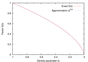
Figure 1: Factor $f\equiv\left(\mathrm{d}\ln D\right)/\left(\mathrm{d}\ln a\right)$ as a function of density parameter $\Omega$ for world models with $\Lambda=0$: exact relation (solid line) and approximation $f\simeq\Omega^{0.6}$ (dashed line).

4 Limit of small $\mathbf{\Omega}$

Let us now examine more thoroughly the limit of $\Omega\to 0$. We begin with checking the asymptotic behaviour of $f(\Omega)$. This regime, although not physically interesting, allows to take a closer look on the bottom-right end of the diagram presented in Fig. 1, and the results obtained will be useful later in the paper. (See also Appendix A.) Starting with the relation (23) and remembering that the limit of small $\Omega$ means $\eta\gg 1$, we get the following approximation:

$$f(\eta)\simeq 6\mathrm{e}^{-\eta}(\eta-3)\qquad(\eta\gg 1)\,.$$ (25)

If we now observe that for such $\eta$ we also have $\eta\simeq\ln 4-\ln\Omega$ and $\mathrm{e}^{\eta}\simeq 4\Omega^{-1}$, we obtain an asymptotic formula for $f(\Omega)$:

$$f(\Omega)\simeq-\frac{3}{2}\Omega(\ln\Omega+3-\ln{4})\qquad(\Omega\ll 1).$$ (26)

Figure 2 clearly shows that for sufficiently small $\Omega$, i.e. $\Omega<0.01$, the power-law of Peebles could no longer be used. This plot is also a confirmation that in some cases the usage of log-log diagrams is well-grounded.

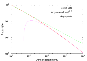
Figure 2: Factor $f(\Omega)$ in the limit $\Omega\ll 1$: exact relation (solid line), power-law approximation (dashed line) and asymptotic relation $f(\Omega)\simeq-(3/2)\Omega(\ln\Omega+3-\ln{4})$ – dotted line. Note logarithmic scales on both axes.

B92 studied the cosmic statistical relation between the non-linear density contrast and the velocity divergence, evolving from Gaussian initial conditions, in the limit of a vanishing variance of the density field. He found the result ‘to be very close to’

$$\Theta^{(\mathrm{B})}=\frac{3}{2}\left[(1+\delta)^{2/3}-1\right]\,.$$ (27)

Here, and from now on, the so-called scaled velocity divergence, $\Theta$, is defined as

$$\Theta=f^{-1}(\Omega)\,\theta\,.$$ (28)

Note that for $|\delta|\ll 1$, the non-linear formula (27) correctly reduces to $\Theta^{(\mathrm{B})}=\delta$, i.e. to the linear-theory relation (19). As already mentioned, B92 claimed his relation to be the same as the one exhibited in the SCM. In turn, B99 argued that the approximation (27) ‘is strictly valid in the limit $\Omega\to 0$’. Here we check these statements, applying the regime $\Omega\ga 0$ to the equations of the SCM.

If $\Omega\ll 1$ then $\eta\gg 1$. Therefore, since for voids ($\delta<0$) we have $\phi>\eta$, also $\phi\gg 1$. For overdensities ($\delta>0$), the limit $\eta\to\infty$ applied to Eq. (13) gives $\delta_{\mathrm{lim}}\to+\infty$. Thus we can focus only on Formula (11) for $\delta$. From Eq. (11) we see that in order to keep $\delta$ finite (though arbitrarily large), also $\phi$ should tend to infinity. In other words, if $\eta\gg 1$, then also $\phi\gg 1$, both for voids and overdensities. Hence, still from Equation (11), we get, up to the leading order,

$$\phi_{1}=\eta-\ln(1+\delta)\;,$$ (29)

and up to the second order

$$\phi_{2}=\eta-\ln(1+\delta)+\left[4(1+\delta)\ln(1+\delta)-\delta(4\eta-6)\right]{\rm e}^{-\eta}.$$ (30)

Equivalently,

$$(1+\delta)\cosh\phi_{2}=\cosh\eta\,+\frac{1}{2}\left[4(1+\delta)\ln(1+\delta)-\delta(4\eta-6)\right]\!.$$ (31)

Applying this formula in Equation (17) and using the large-$\eta$ limit of the function $f(\eta)$ (Eq. 25) we obtain

$$\Theta\,\simeq\,\delta-\frac{N(\delta)}{\eta-3}\;\simeq\;\delta+\frac{N(\delta)}{\ln\Omega+3-\ln 4}\,,$$ (32)

where

$$N(\delta)=(\delta+1)\ln(\delta+1)-\delta\,.$$ (33)

In the limit $\Omega\to 0$ the second term in Equation (32) vanishes, hence

$$\Theta=\delta\,.$$ (34)

This is exactly the same relation as for the linear regime (where $|\delta|\ll 1$). However, here the density contrast can have an arbitrary value. Thus, the formula of B92  (27) does not describe the dynamics of perturbations in the limit $\Omega\to 0$. The relation (34), being very simple, is a non-trivial result. When $\Omega$ tends to 0, then also the (not scaled) velocity divergence $\theta\to 0$ (peculiar velocities vanish with diminishing $\Omega$). However, the quantity $\Theta$, as introduced by Eq. (28), converges to a non-zero value for $\Omega\to 0$, due to the presence of the factor $f(\Omega)$, approximated by (26) for small $\Omega$. The normalisation used here leads to $\Theta=\delta$ in the linear theory. Why for very small values of $\Omega$ this relation holds also in the non-linear regime? It turns out that this is a general result of dynamics in a low-density universe, and does not rely on any symmetry. The derivation is presented in Appendix A.

For large but finite values of $\eta$, Formula (32) can be applied. Specifically, it can be used for $\eta$ significantly greater than 3 ($\Omega$ significantly smaller than $0.2$), which falls well below the presently accepted value of the cosmic density parameter. Therefore, the approximation (32) is of no practical importance; we have to continue our search for a relevant relation. Just for illustrative purposes, on Figure 3 we plot the exact relation, the B92 approximation, and the approximation (32), for an exemplary value of $\Omega=10^{-5}$ ($\eta\simeq 13$). We see that although for this value of $\Omega$ the relation is still non-linear, the B92 approximation drastically overestimates the degree of non-linearity.

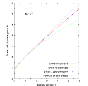
Figure 3: A comparison of the relation between density contrast $\delta$ and scaled velocity divergence $\Theta=f^{-1}\,\theta$ for very small $\Omega$ (here $\Omega=10^{-5}$): linear theory result $\Theta=\delta$ – dotted line, exact relation $\Theta(\delta)$ – solid line, approximation for small $\Omega$ – crosses and B92 approximation (27) – dashed line.

5 Relations for voids

As voids we will understand any underdense perturbations, i.e. those for which $\delta<0$. In this section we examine the behaviour of the velocity divergence vs. the density contrast for such inhomogeneities.

When considering overdense perturbations (with $\delta>0$), the regime of $\delta\simeq 1$ is usually called weakly (or at most mildly) non-linear. It may thus seem that it should be similarly for the limit $\delta\ga-1$ (cf. Martel 1991). However, if we analyse Equation (11), which is valid both for voids and for open overdensities, we can see that for finite values of $\eta$ (which correspond to non-zero $\Omega$), the condition $\delta\to-1$ may only be satisfied for $\phi\to+\infty$. Hence, the evolution of such a perturbation is highly non-linear when the density contrast approaches its minimum value.

The scaled velocity divergence $\Theta$, as defined in Eq. (28), is a monotonically increasing function of $\delta$ (for $\eta$, or $\Omega$, treated as a fixed parameter). Its minimum value is $\Theta_{\mathrm{min}}\equiv\Theta(-1)$ (dependent on $\eta$), obtained easily by calculating the limit $\phi\to+\infty$ in (15):

$$\Theta_{\mathrm{min}}=3f^{-1}(\eta)\left[1-\frac{(\cosh\eta-1)^{2}}{\sinh\eta\,(\sinh\eta-\eta)}\right].$$ (35)

For $\eta\to 0$, equivalent to $\Omega\to 1$ (the Einstein–de Sitter model of the universe), we get the value of $\Theta_{\mathrm{min}}=-1.5$, which can also be calculated otherwise. The opposite limit of $\Omega\to 0$ ($\eta\to+\infty$) leads to $\Theta_{\mathrm{min}}\to-1$; this can be equally deduced from (34). If we adopt the currently accepted value of $\Omega_{0}\simeq 0.25$ ($\eta_{0}\simeq 2.63$), we obtain $\Theta(-1)\simeq-1.43$. Thus, the B92 approximation (27), which gives $\Theta(-1)=-1.5$ independently of $\Omega$, has a relative error of approx. 5% in this limit for such $\Omega_{0}$.

We would now like to find an (approximate) relation $\Theta$–$\delta$ for the whole range $\delta\in[-1,0]$. B92 derived his formula expanding the relation around $\delta=0$. We adopt a different approach: we expand the relation around $\delta=-1$. (That is, at a first step we assume $0\leq\delta+1\ll 1$). Then, for arbitrary $\eta$, the perturbation parameter $\phi\gg 1$. From Equation (11) we obtain $\cosh\phi_{1}=g(\eta)/(1+\delta)$, where

$$g(\eta)=\frac{(\cosh\eta-1)^{3}}{(\sinh\eta-\eta)^{2}}\,,$$ (36)

and further on

$$\cosh\phi_{2}=\cosh\phi_{1}+3-2\phi_{1}\,.$$ (37)

Using Equation (37) in Equation (17) we get

$$\Theta_{2}=\Theta_{\rm min}+f^{-1}(\eta)\frac{3\,(\sinh\eta-\eta)\,(\phi_{1}-2)}{\sinh\eta\,(\cosh\eta-1)}\,(1+\delta)\,,$$ (38)

where

$$\phi_{1}=\ln\left[2g(\eta)\right]-\ln(1+\delta)\,.$$ (39)

Equation (38) satisfies explicitly the highly non-linear limit $\Theta(-1)=\Theta_{\rm min}$. Also, in the limit $\eta\gg 1$, this Equation reduces to asymptotic Equation (32), as expected.

The range of applicability of formula (38) is very limited: it starts to deviate from the exact relation for $\delta$ about $-0.9$. We would like to introduce such a modification so as to satisfy also the linear-theory limit: for $|\delta|\ll 1$, $\Theta=\delta$. Therefore, we adopt the following three boundary conditions:

1. $\Theta(-1)=\Theta_{\rm min}$,

2. $\Theta(0)=0$,

3. $\left(\mathrm{d}\Theta/\mathrm{d}\delta\right)|_{\delta=0}=1$.

Inspired by Equation (38), we write

$$\Theta=\Theta_{\rm min}+a_{1}(\eta)(1+\delta)+a_{2}(\eta)(1+\delta)\ln(1+\delta)\,,$$ (40)

where $a_{1}$ and $a_{2}$ are arbitrary functions of $\eta$. Imposing the three boundary conditions A.–C. on the above formula we find

$$\Theta=\delta+(1+\Theta_{\mathrm{min}})\,N(\delta)\,,$$ (41)

where $\Theta_{\mathrm{min}}$ as a function of $\Omega$ [cf. (42)] is

$$\Theta_{\mathrm{min}}(\Omega)=3\,f^{-1}(\Omega)\,\times$$

$$\times\left\{1-\frac{2\sqrt{(1-\Omega)^{3}}}{2\sqrt{1-\Omega}-\Omega\ln[2\Omega^{-1}(1+\sqrt{1-\Omega})-1]}\right\}\simeq$$

$$\simeq\,-1-0.5\Omega^{0.12-0.06\,\Omega}$$ (42)

[here $f(\Omega)$ is given by (24)] and $N(\delta)$ has the form of (33). Indeed, formula (41) meets all the three boundary conditions: the last two are fulfilled since for small $\delta$, $N(\delta)=\delta^{2}/2+\ldots$, and the first one because $N(-1)=1$. This simple approximation is robust for $\delta$ close to $-1$ and around $0$; for intermediate values of $\delta$ it slightly underestimates the exact value of $\Theta$ (with a maximal relative error of 2% for $\Omega\simeq 0.25$).

Formula (41) is probably already sufficiently accurate for practical applications. Still, it is of course possible to improve it. In order to do this, we expand the exact $\Theta$–$\delta$ relation around $\delta=-1$ up to third-order in the perturbation parameter $\phi$. The result is the following series:

$$\Theta_{3}=a_{0}+a_{1}(1+\delta)+a_{2}(1+\delta)\ln(1+\delta)+a_{3}(1+\delta)^{2}$$

$$+\,a_{4}(1+\delta)^{2}\ln(1+\delta)+a_{5}(1+\delta)^{2}\ln^{2}(1+\delta),$$ (43)

where $a_{i}$ are some functions of $\eta$ (see Appendix B). From the six terms above we construct their linear combinations which fulfill the constraints A.–C. This, together with the condition of simplicity, leads us to postulate

$$\Theta=\delta+\left[1+\Theta_{\mathrm{min}}(\Omega)\right]N(\delta)+\alpha_{1}(\Omega)\,\delta\,(1+\delta)\ln(1+\delta)\,+\,$$

$$\alpha_{2}(\Omega)(1+\delta)^{2}\ln^{2}(1+\delta)\,,\hphantom{x}$$ (44)

Fitting this formula to the exact relation gives $\alpha_{1}=0.12$ and $\alpha_{2}=-0.09$ for $\Omega=0.25$. The fit is very accurate: it has a maximal error smaller than $0.2$%. In general, both $\alpha_{1}$ and $\alpha_{2}$ depend weakly on $\Omega$: we have $\alpha_{1}\simeq 0.19\,\Omega^{0.35}$ and $\alpha_{2}\simeq-0.15\,\Omega^{0.35}$ for $0.1\leq\Omega\leq 0.9$. Figure 4 presents a comparison of the exact relation for $\Theta(\delta)$, calculated for voids from (17), with the fit (44) and the B92 approximation (27). As we can see, our fit lies accurately on the approximated curve and the B92 formula slightly underestimates exact values of $\Theta$ for $\delta$ close to $-1$. However, it should be admitted that the latter is considerably simpler than ours.

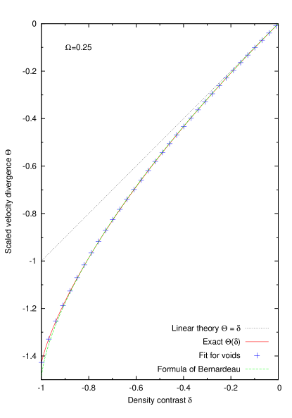
Figure 4: Relation between density contrast and scaled velocity divergence for spherical voids (underdensities): linear theory (dotted line), exact relation (solid line), B92 approximation (dashed line) and fit given by Equation (44) (crosses). The density parameter of the background is $\Omega=0.25$.

6 Overdensities

An overdensity is any perturbation for which $\delta>0$. As already mentioned, these can be of two types, depending on the initial density contrast: ‘open’ or ‘closed’. For a specific value of $\Omega$ (or, equally, $\eta$), the boundary value of the density contrast, maximal for the first type and minimal for the second, is given by (13). For the currently accepted value of $\Omega_{0}\simeq 0.25$ we have $\delta_{\mathrm{lim}}\simeq 1.6$: such overdense but open perturbations ($\delta<\delta_{\mathrm{lim}}$) fall within the weakly non-linear regime.

In order to find an approximation for $\Theta(\delta)$ for overdense spherical regions, we will use a similar procedure as we did for voids, examining the highly non-linear regime ($\delta\gg 1$). Owing to the considerations above, it is sufficient to focus on closed perturbations; the formula for $\Theta$ is then of the form (18), with the ‘+’ sign. Highly non-linear infall means that the overdensity collapses to a point: the conformal time of the perturbation $\phi\to 2\pi$. This is in general not physical, as in practice for $\phi\la 2\pi$ virialisation would occur and prevent further collapse. However, as in the case of voids, examination of this regime leads to interesting formulae.

First of all, we can directly put $\phi=2\pi$ into (18), getting the ‘1-st order approximation’:

$$\Theta_{1}=3f^{-1}(\Omega)\left[1+\sqrt{\Omega(1+\delta)}\right]\,.$$ (45)

We can see that the B92 formula (27), which was not intended to work in this regime, indeed will not work: already the slope of the curve is incorrect (2/3 instead of 1/2). For realistic values of $\Omega$, $f^{-1}(\Omega)\sqrt{\Omega}\simeq\Omega^{-0.1}$. Using this approximate equality and neglecting the constant term in Equation (45) yields the ‘0-th order approximation’, $\Theta_{0}=3\,\Omega^{-0.1}\sqrt{1+\delta}$. The same relation can be deduced from dynamical considerations (namely, from energy conservation in the highly non-linear infall). NuCo98 also found such a form of the weak $\Omega$-dependence $\left(\Omega^{-0.1}\right)$ of the peculiar velocity in virialised regions. This is not surprising, since both in our and their case, $\delta\gg 1$ and $\Theta\ll\delta$.

Expanding the relation (18) around $\phi=2\pi$ ($0\leq 2\pi-\phi\ll 1$) to higher order, we obtain the following series:

$$\Theta=3f^{-1}(\Omega)\big{[}1+\sqrt{\Omega}(1+\delta)^{1/2}+a_{1/6}\sqrt{\Omega}(1+\delta)^{1/6}+$$

$$+a_{-1/6}\sqrt{\Omega}(1+\delta)^{-1/6}+\cdots\big{]}\,,$$ (46)

where $a_{\mathrm{i}}$ are functions of $\Omega$ only. In order to obtain a fit that would both converge to (45) in the highly non-linear regime of $\delta\gg 1$ and have proper behaviour in the vicinity of $\delta=0$ (conditions B. and C. from Section 5), we proceed similarly as we did for $\delta<0$. First, already here we neglect the fourth (and all next) component of the series. Then we modify the expansion (6) by introducing two parameters $\mathcal{A}$, $\mathcal{B}$ and an integer $n$:

$$\Theta=3f^{-1}\left[\mathcal{A}+\sqrt{\Omega}\sqrt{1+\delta}-\mathcal{B}\sqrt{\Omega}(1+\delta)^{1/n}\right].$$ (47)

Imposing the conditions $\Theta(0)=0$ and $\left(\mathrm{d}\Theta/\mathrm{d}\delta\right)|_{\delta=0}=1$, we obtain:

$$\mathcal{A}=\left(\frac{n}{2}-1\right)\sqrt{\Omega}-\frac{n}{3}f(\Omega)\,,\qquad\mathcal{B}=\frac{n}{2}-\frac{n}{3\sqrt{\Omega}}f(\Omega)\,.$$ (48)

In particular, for $n=6$ [cf. (6)] we have

$$\mathcal{A}(\Omega,n=6)\simeq 2\Omega^{0.5}\!\left(1-\Omega^{0.1}\right),$$ (49)

and

$$\mathcal{B}(\Omega,n=6)\simeq 3-2\Omega^{0.1}$$ (50)

(remembering that $f\simeq\Omega^{0.6}$). Inserting the above expressions for $\mathcal{A}$ and $\mathcal{B}$ into Equation (47) with $n=6$ and neglecting the weak $\Omega$-dependence [since $f^{-1}(\Omega)\sqrt{\Omega}\simeq\Omega^{-0.1}$], we obtain the following result, which can be treated as a generalisation of the B92 formula:

$$\Theta=3\left[(1+\delta)^{1/2}-(1+\delta)^{1/6}\right]\,.$$ (51)

An interesting feature of this fit is that it has the same second-order Taylor expansion around $\delta=0$ as the approximation given by B92 :

$$\Theta=\delta-\frac{1}{6}\delta^{2}+\cdots\,.$$ (52)

This means that in the weakly non-linear regime these two approximations give similar results. However, for mildly non-linear values of $\delta$ (from $\delta_{\mathrm{lim}}$ up to the turn-around) our approximation works generally better than the formula of B92 . The maximal error of our fit for such an interval of density contrasts is about 1.5%. Figure 5 shows the discussed approximations for the weakly and mildly non-linear regime.

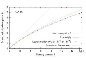
Figure 5: A comparison of proposed approximations for $\Theta(\delta)$ with the exact relation for spherical overdensities in the mildly non-linear regime (up to the turn-around). Solid line shows the exact relation, the B92 approximation (27) is illustrated by dashed line and crosses present the fit given by (51); dotted line is the linear theory relation. The density parameter of the background equals to $\Omega_{0}=0.25$; the density contrast of the turn-around is then $\delta_{\mathrm{ta}}\simeq 13.5$.

For higher values of $\delta$, neither the B92 approximation, nor the fit (51) are adequate. In case of the first one this is mainly due to a wrong slope of the curve; in case of the second – due to the negligence of the dependence on $\Omega$. For that reason in the regime of very big $\delta$ we prefer to use the fit (47), of a more general form. The approximation (51) suggests that the best choice of $n$ is $n=6$; however, it turns out that in practice, for highly non-linear density contrasts (greater than the value for the turn-around), approximation (47) with $n=4$ works slightly better than with $n=6$ (with the weak $\Omega$-dependence included in both cases). In Figure 6 we show the behaviour of the function $\Theta(\delta)$ in the highly non-linear regime. For comparison, we plot the formula of B92 , the simple approximation (51) and the approximation (47) with $n=4$.

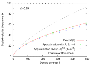
Figure 6: An illustration of the behaviour of the function $\Theta(\delta)$ for spherical overdensities in the highly non-linear regime, i.e. up to the virialisation. The solid curve is the exact relation, the dashed line shows the B92 approximation and crosses present two approximations described in the text: plus marks represent the formula (51) and multiplication marks show the fit (47) with $n=4$.

Our results for the highly non-linear regime are rather of academic value, since, as stated earlier, highly non-linear infall is considerably modified by the effects of virialisation. To account for them (and for deviations from spherical symmetry), Shaw & Mota (2008) constructed an improved (extended) semi-analytical spherical collapse model. For $\delta$ up to about $\delta_{\mathrm{ta}}$ (which equals to $\sim 4.6$, as the background assumed in the discussed paper is of the Einstein–de Sitter type) their model coincides with the standard spherical model (studied here), while for larger density contrasts it deviates from the latter and under some additional assumptions matches well the results of N-body simulations presented by Hamilton et al. (1991). Indeed, formula (20) of Shaw & Mota (2008), for $T=\tau$ (the limit of the standard model), reduces to our Equation (18) (their $h_{\mathrm{SC}}=\theta/3$). The authors argue that for background universes with dark energy their formula is valid only for $\delta\ga 100$. They claim that for smaller values of $\delta$, their results are not accurate. We disagree with these statements. As already stated, the weak $\Omega$ and $\Lambda$ dependence of the scaled velocity–density relation has been shown on the level of the equations of motion (NuCo98, ), so independently of the level of non-linearity. Since for small redshifts dark energy behaves similarly to the cosmological constant (e.g. Riess et al. 2007), and since only for such redshifts the weak dependence of equations of motion on cosmological parameters starts to play any role (because earlier we had $\Omega\la 1$; NuCo98 ), the velocity–density relations for cosmological models with and without dark energy must be similar.

7 Comparisons with fits to numerical simulations

KaCPeR00 studied the mildly non-linear velocity–density relation using the Cosmological Pressureless Parabolic Advection (CPPA) hydrodynamical code. They found that the mean relation between the scaled velocity divergence and the density contrast can be very well described by the so-called ‘$\gamma$-formula’,

$$\Theta=\gamma\left[(1+\delta)^{1/\gamma}-1\right]+{\epsilon}\,,$$ (53)

with $\gamma\simeq 1.9$. This formula is a modification of the B92 formula with $\gamma$ instead of $3/2$. The offset ${\epsilon}>0$ is introduced to account for an effect of a finite variance of the density field: the value of ${\epsilon}$ is such that the global mean of $\Theta$ is zero, as required. (Another effect of a finite variance is to modify the degree of non-linearity of the relation.) Without the offset, the above formula yields $\Theta(-1)=-\gamma=-1.9$ for $\gamma=1.9$, in significant difference with the value $-1.5$, obtained neglecting the weak $\Omega$-dependence of the exact limit, Eq. (35). However, for Gaussian smoothing scales of a few Mpc, employed in KaCPeR00 , the offset shifts the value of $\Theta(-1)$ much closer to $-1.5$.

B99 analysed the velocity–density relation using N-body simulations performed for various background cosmologies. They noticed a weak dependence of the relation on $\Omega$ and $\Lambda$. B99 invented a somewhat more elaborate fit to the extracted mean relation, presented in the form of density in terms of velocity divergence,

$$\delta=\beta\left(1+\Theta/\gamma\right)^{\gamma}-1\,.$$ (54)

Here, $\beta$, slightly smaller than unity, plays a role of the offset ${\epsilon}$ in Equation (53): it assures that the global mean of $\delta$ is zero, as required. In Equation (54) $\gamma$ is not a constant, but is approximated as a following function of $\Theta$:

$$\gamma=\frac{3}{2}+0.3\,\Omega^{0.6}\left(\Theta+\frac{3}{2}\right)\,.$$ (55)

The above equation quantifies the fact that for larger values of velocity divergence, the observed relation becomes more non-linear. Indeed, $\gamma$ grows with growing $\Theta$ (we recall that $\gamma=1$ corresponds to the linear theory). Moreover, for $\Theta=-3/2$, we have $\gamma=3/2$, so then $\delta=-1$, as it was intended. [Note a typo in eq. (20) of B99 : instead of $\tilde{\theta}$ (in our notation, $\Theta$), there should be $\theta$.]

How do these findings, based on fully non-linear simulations, relate to our results? In overdensities, our Formula (51) follows closer to the exact relation in the SCM than the formula of B92 . Moreover, our approximation is a formula with increasing effective index $\gamma_{\rm eff}$. Its second order expansion is the same as that of B92 , so for small $\delta$, $\gamma_{\rm eff}=3/2$. For large density contrasts, the second term in Equation (51) becomes negligible, so asymptotically $\gamma_{\rm eff}=2$ (for $\delta\gg 1$). Therefore, qualitatively our formula is consistent with the fit of B99 , in a sense that $\gamma$, as a function of $\Theta$ or $\delta$, is growing. It is also consistent with the fit of KaCPeR00 , in a sense that the average $\gamma$ is slightly larger than $3/2$. Clearly, our formula is a better fit to the results of numerical simulations than the formula of B92 .

Of course, quantitatively there are discrepancies. First of all, it is strictly impossible to satisfy simultaneously the features of both fits: $\gamma$ is either constant or increasing. This discrepancy between the results of the two groups is not necessarily a sign of a major flaw in any of their analyses. The two groups used different codes: N-body versus hydro. The first one follows accurately non-linear evolution, but provides naturally a mass-, not volume-, weighted velocity field, while the latter is needed. CPPA, as any hydrodynamical code, provides naturally a volume-weighted velocity field, but follows the non-linear evolution after shell crossings only approximately. Moreover, the density power spectra used in both simulations were different. Also, fit (54) of B99 was found for top-hat smoothed fields, while fit (53) of KaCPeR00 was elaborated for fields smoothed with a Gaussian filter (more appropriate for velocity–density comparisons). The effects of smoothing, though small, are different for these two filters (see e.g. Table 1 of KaCPeR00 ). Finally, an inverse of the forward relation (density in terms of velocity divergence) does not strictly describe the mean inverse relation, due to scatter.

Which results better reflect real non-linear dynamics of cosmic random density and velocity fields? Instead of betting, it would be probably best to repeat the analysis using an output from high-resolution N-body simulations with a $\Lambda$CDM power spectrum, employing – instead of a Voronoi tessellation (Bernardeau & van de Weygaert, 1996) – a much simpler algorithm of extracting volume-weighted velocity field of Colombi, Chodorowski & Teyssier (2007). Voronoi tessellations are complicated and very CPU-consuming, so they can be applied only to a limited number of points, while the method of Colombi et al. (2007) can be (and actually has been) applied to all simulation points ($512^{3}$ in their work). If the actual relation is not more non-linear than in the highly non-linear regime of the SCM ($\gamma=2$), then we can use Formula (47), with neglected weak $\Omega$-dependence and $n$ treated as a free parameter. Let us write it explicitly:

$$\Theta^{(2,n)}=3\left[(1+\delta)^{1/2}-\frac{n}{6}(1+\delta)^{1/n}\right]+{\epsilon}\,,$$ (56)

where ${\epsilon}=n/2-3$. [For $n=6$, it reduces to Formula (51).] For example, if the best-fit value of $\gamma$ is found to be close to $1.9$ and fairly constant, then $n=2.3$ would provide an excellent fit. Instead, significant ‘run’ of the index $\gamma$ would probably demand $n>6$.

If, on the other hand, the results of B99 are found to be accurate, then for $\Omega=0.25$ Equation (55) yields $\gamma=2$ already for $\Theta\simeq 2.3$, and even more for higher $\Theta$. In this case, in order to describe the relation up to the turn-around, one should modify also the exponent of the leading term in Formula (56) ($1/m$ instead of $1/2$, with $m\ga 2$). It is a matter of choice if to fit one ‘running’ exponent ($\gamma$) or two constant ($m$ and $n$). In any case, it is better to use an additive offset ${\epsilon}$ instead of the factor $\beta$, appearing in Equation (54): in applications to velocity–velocity comparisons the value of ${\epsilon}$ is not relevant at all. The mildly non-linear velocity field is vorticity-free to good accuracy, so the predicted velocity field (from the density field) is

$${\bf v}({\bf r})=\frac{Hf(\Omega)}{4\pi}\!\!\int\!{\rm d}^{3}{\bf r}^{\prime}\,\,\frac{\Theta[\delta({\bf r}^{\prime})]\,({\bf r}^{\prime}-{\bf r})}{|{\bf r}^{\prime}-{\bf r}|^{3}}\,,$$ (57)

and the contribution of the offset to velocity averages out to zero.

An advantage of the $\gamma$-formula over Formula (56) or its modification is that it works also for voids. For underdensities, the formula of B92 is a very good description of the exact relation in the SCM, except for the very tail $\delta\simeq-1$ (where the weak $\Omega$-dependence becomes important). Results of numerical simulations show very limited need to modify the formula of B92 for voids – the discrepancies appear at larger density contrasts. As stated earlier, B92 predicted this fact. Our formulae for voids give results very similar to that of B92 , but describe better the regime $\delta\simeq-1$. This regime is important for predicting expansion velocities of almost completely empty voids (e.g., see Tully et al. 2008). Therefore, using approximation (41) for underdensities, we propose the following combined formula:

$$\Theta=\left\{\begin{array}[]{lr}\Theta^{(m,n)}\,,&\delta>0,\\ \delta-0.5\,\Omega^{0.12-0.06\,\Omega}N(\delta)+{\epsilon}\,,&-1\leq\delta\leq 0\,.\end{array}\right.$$ (58)

Here, $\Theta^{(m,n)}$ is the ‘$m$-modification’ of Formula (56), $N(\delta)$ is given by Equation (33) and ${\epsilon}$, treated as a free parameter, is the same in both cases. Alternatively, as the relation for voids, one could use more complicated and extremely accurate Equation (44). To sum up, we admit that it is disputable if to fit results of numerical simulations using our formula (58), or $\gamma$-formula. What remains indisputable is that for overdensities, our standard formula (with $m=2$ and $n=6$) is a better starting fit than the standard formula of B92 (with $\gamma=3/2$).

8 Summary and conclusions

The main motivation of this paper was to rederive the formula of B92 in a simple way, using the spherical collapse model (SCM), and to extend it to larger density contrasts, where it is no longer valid. The undertaken project abounded in surprises:

1. Contrary to the claim of B99 , the formula of B92 is not exact in the limit of an empty universe. On the contrary, it completely fails in this regime: the exact relation in the SCM is then $f^{-1}\nabla\cdot\mathbf{v}=\delta$, for an arbitrary $\delta$. In fact, this is a general result of dynamics in a low-density universe.

2. Although the formula of B92 fails for $\Omega\to 0$, where it was expected to work best, for realistic values of $\Omega$ (say, $\Omega>0.1$), it describes very well the SCM velocity–density relation in voids. It also works for overdensities up to $\delta\sim 2$ – $3$.

The velocity–density relation in the SCM is given in a parametric form. Our goal here was to eliminate this parameter (at least approximately) and to provide the relation analytically. We aimed at describing the relation in the whole range $\rho\in(0,\infty)$ (realistically, up to $\rho_{\rm vir}$). Therefore, instead of expanding it around $\rho=\rho_{\rm b}$, we adopted an entirely different approach. Namely, we derived asymptotes of the relation in the highly non-linear regime: $\rho/\rho_{\rm b}\gg 1$ ($\delta\gg 1$) for overdensities and $\rho_{\rm b}/\rho\gg 1$ ($0\leq 1+\delta\ll 1$) for voids. (Although we also ‘expanded’ around them, in a sense that we also calculated next-to leading-order terms.) These two asymptotes turned out to be qualitatively different. Inspired by their functional forms, we invented semi-phenomenological fits to the exact relation (separately for overdensities and voids), fulfilling the linear theory condition $f^{-1}\nabla\cdot\mathbf{v}=\delta$.
For overdensities, our main result is Formula (51). It describes well the exact relation in the SCM up to the turn-around (for $\Omega=0.25$, $\delta_{\rm ta}=13.5$). As already stated, the formula of B92 starts to deviate from the exact relation for $\delta\sim 3$. We have also fitted the regime $\delta\in(\delta_{\rm ta},\delta_{\rm vir})$, though virialisation and departures from spherical symmetry make practical applicability of the SCM in this regime very limited.
In case of voids, the most important results of this paper are Formulae (41) and (44), with $\Theta_{\mathrm{min}}$ given by Equation (42). Compared with the SCM, simple Formula (41) has a maximal error of about $2$% and is probably sufficient for practical applications. The formula of B92 is an even better approximation, except for the limit $\delta\to-1$, where for $\Omega=0.25$ it has approximately $5$% relative error. Our more complicated formula (44) is extremely accurate in the whole range $\delta\leq 0$: its maximal error is about $0.2$%.
An ultimate goal of studies such as the present one is to find the relation valid for realistic random cosmic velocity and density fields. Unlike the work of B92 , our calculations were greatly simplified by the strong assumption of spherical symmetry. There is therefore no guarantee that better agreement with the SCM implies better agreement with the real relation. In order to check this issue we compared our formulae to fits to results of cosmological numerical simulations, that are present in the literature. We have found that in voids, our formulae, as well as the formula of B92 , describe well the real relation. This is partly a consequence of the fact that voids are more spherical than overdensities. In overdensities, both our formula and that of B92 require modification, but ours less. This discrepancy is not a failure of the latter of the two, since it has never been intended to work for $\delta\ga 2$. Our formula (51), having the same second-order expansion as the formula of B92 , can be regarded as its extension into the mildly non-linear regime (for $\delta$ up to the turn-around). We have also discussed how to (slightly) modify our formula to better fit numerical simulations.
In Section 1 we have enlisted arguments for weak dependence of the velocity–density relation on the cosmological parameters. Therefore, in the present analysis we set $\Lambda=0$. To study the limit $\Omega\to 0$ we have retained $\Omega$-dependence of the equations of the SCM. Analysing these equations we have confirmed that for realistic values of $\Omega$, the $\Omega$-dependence of the relation is indeed very weak. In final formulae it has been therefore neglected, except for Formula (42) for $\Theta_{\mathrm{min}}$. The difference between $\Theta_{\mathrm{min}}$ for $\Omega=1$ and $\Omega=0.25$ is about $5$%. In fact, if we want to have better accuracy, there is no guarantee that $\Lambda$ does not contribute at a comparable level. It is then worth to repeat the analysis with $\Lambda=1-\Omega$. We plan to undertake such a study in the future.

Appendix A The velocity–density relation in an empty universe

The general equation of motion for the cosmic pressureless fluid in comoving coordinates is

$$\frac{\partial{\bf v}}{\partial t}+\frac{1}{a}\left({\bf v}\cdot\nabla\right){\bf v}+\frac{\dot{a}}{a}{\bf v}={\bf g}\,,$$ (59)

where ${\bf g}$ is the peculiar gravitational acceleration,

$${\bf g}({\bf x},t)=G\rho_{\rm b}a\!\!\int\!{\rm d}^{3}{\bf x}^{\prime}\,\,\frac{\delta({\bf x}^{\prime},t)\,({\bf x}^{\prime}-{\bf x})}{|{\bf x}^{\prime}-{\bf x}|^{3}}$$ (60)

(e.g. Peebles 1980). For $|\delta|\ll 1$ we can neglect the non-linear term on the LHS of Equation (59). Let us choose some instant of time, $t_{i}$, of the evolution of an open universe when already $\Omega\ll 1$. For such $\Omega$ perturbations stop growing, so for $t>t_{i}$, ${\bf g}({\bf x},t)={\bf g}_{i}({\bf x})/a^{2}$. Our Equation (59) simplifies then to

$$\frac{\partial}{\partial t}[a\,{\bf v}({\bf x},t)]=\frac{{\bf g}_{i}({\bf x})}{a}.$$ (61)

The solution is

$${\bf v}({\bf x},t)=H_{0}^{-1}(\eta-\eta_{i})\frac{{\bf g}_{i}({\bf x})}{a(t)}+\frac{{\bf v}_{i}({\bf x})}{a(t)}+\frac{\mn@boldsymbol{F}({\bf x})}{a(t)},$$ (62)

where the conformal time $\eta$ is in general defined in Equation (3). The last term in Equation (62) is the homogeneous part. Here we do not assume a priori irrotationality of the velocity field, so we retain this term. (Though it does not contribute to the velocity divergence, because $\nabla\cdot\mn@boldsymbol{F}=0$.) The limit $\Omega\to 0$ corresponds to $\eta\to\infty$. Therefore, in the above equation we can neglect the terms ${\bf v}_{i}/a$ and $\mn@boldsymbol{F}/a$, as well as $\eta_{i}$. This yields

$${\bf v}=H_{0}^{-1}\eta\,a\,{\bf g}\,.$$ (63)

From Equation (60) we have

$$\nabla\cdot{\bf g}=-4\pi G\rho_{\rm b}a\delta=-\frac{3}{2}H^{2}\Omega a\delta\,.$$ (64)

This yields in (63)

$$\nabla\cdot{\bf v}=-\frac{3}{2}H_{0}^{-1}(Ha)^{2}\Omega\eta\,\delta\,.$$ (65)

In an (almost) empty universe $H(t)=t^{-1}$ and $a(t)=t/t_{0}$, hence $Ha=H_{0}$. Also, the general relation (5) between $\Omega$ and the conformal time simplifies then to $\Omega=4{\rm e}^{-\eta}$. Substituting this in Equation (65) we obtain $\nabla\cdot{\bf v}=-H_{0}6\eta{\rm e}^{-\eta}\delta$. Comparing this equation with Equation (25), we identify the factor $6\eta{\rm e}^{-\eta}$ as the low-$\Omega$ limit of the factor $f(\Omega)$. Hence,

$$\nabla\cdot{\bf v}=-H_{0}f(\Omega)\,\delta\,,$$ (66)

in agreement with the general linear theory prediction, Equation (1).

Now, we claim that in the limit $\Omega\to 0$, solution (63) is also a solution of the general equation of motion (59), for arbitrary $\delta$. To prove this statement we have to demonstrate that in this limit, the non-linear term in equation (59) is negligible. Substituting solution (63) in this term gives

$$\frac{\partial{\bf v}}{\partial t}+\frac{\dot{a}}{a}{\bf v}={\bf g}-\frac{1}{a}\left(H_{0}^{-1}\eta a{\bf g}\cdot\nabla\right)(H_{0}^{-1}\eta a{\bf g})\,.$$ (67)

The amplitude of the second term on the RHS is of order $H_{0}^{-2}\eta^{2}a\,g\,\nabla\cdot{\bf g}\sim H_{0}^{-2}\eta^{2}a\,g\,H^{2}\Omega a\,\delta$. The amplitude of the second term relative to the first is thus

$$\frac{2\mathrm{nd}}{1\mathrm{st}}\sim H_{0}^{-2}(Ha)^{2}\eta^{2}\Omega\,\delta\sim\eta^{2}\Omega\,\delta\sim\eta^{2}{\rm e}^{-\eta}\delta\,,$$ (68)

and in the limit $\Omega\to 0$ it tends to zero. (Formally speaking, for arbitrary ${\epsilon}>0$ and arbitrary $\delta$, there always exists $\eta_{\epsilon}$ such that for all $\eta>\eta_{\epsilon}$, $\eta^{2}{\rm e}^{-\eta}|\delta|<{\epsilon}$.) Thus, in the limit $\Omega\to 0$ the non-linear term in the equation of motion becomes negligible, for arbitrary value of $\delta$. This is why in every matter-only, open universe, the velocity–density relation evolves towards the linear one.

Appendix B Third-order expansion for $\mn@boldsymbol{\Theta}$ in voids

Our aim here is to extend calculations of Section 5 for voids up to third order in the perturbation parameter $\phi$ ($\phi$ is assumed to be large, but not infinitely large). We begin applying to Equation (11) the equality $\sinh\phi=\cosh\phi\,-\,\exp(-\phi)$ and expand this equation up to terms of the order $\cosh^{-2}\phi$. Solving perturbatively the resulting equation for $\phi_{3}$ we obtain

$$\cosh\phi_{3}=\cosh\phi_{2}-\frac{3\phi_{1}^{2}-10\phi_{1}+10}{\cosh\phi_{1}}\,,$$ (69)

where $\cosh\phi_{2}$ is given by Equation (37), $\phi_{1}$ by (39) and the second term on the RHS of the above equation is a small correction. This enables us to write

$$\sqrt{1+\cosh\phi_{3}}\simeq\sqrt{1+\cosh\phi_{2}}-\frac{3\phi_{1}^{2}-10\phi_{1}+10}{2\,\cosh^{3/2}\phi_{1}}\,.$$ (70)

Using the above equation in Equation (17) yields

$$\Theta_{3}=\Theta_{2}+\frac{3}{2}\sqrt{\frac{\Omega}{2}}\frac{(\sinh\eta-\eta)^{3}}{(\cosh\eta-1)^{9/2}}\left(3\phi_{1}^{2}-10\phi_{1}+10\right)\times$$

$$(1+\delta)^{2},~{}$$ (71)

or, finally,

$$\Theta_{3}=\Theta_{2}+\frac{3\,(\sinh\eta-\eta)^{3}}{2\,\sinh\eta\,(\cosh\eta-1)^{4}}\,F(\delta,\eta)\,(1+\delta)^{2}\,.$$ (72)

Here,

$$F(\delta,\eta)=3\ln^{2}(1+\delta)\!\!\!\!\! + \!\!\!\!\![10-6\ln(2g)]\,\ln(1+\delta)+3\ln^{2}(2g)$$ (73)

$$- \!\!\!\!\!10\ln(2g)+10\,,$$

and $g(\eta)$ is given by Equation (36). Inspecting terms in the above equation we see that Equation (72) can be indeed written in the form (43).

References

- (1) Bernardeau F., 1992, ApJ, 390, L61-L64 (B92)
- (2) Bernardeau F., Chodorowski M.J., Łokas E.L., Stompor R., Kudlicki A., 1999, MNRAS, 309, 543-555 (B99)
- Bernardeau & van de Weygaert (1996) Bernardeau F., van de Weygaert R., 1996, MNRAS, 279, 693-711
- Bouchet et al. (1995) Bouchet F.R., Colombi S., Hivon E., Juszkiewicz R., 1995, A&A, 296, 575-608
- Catelan et al. (1995) Catelan P., Lucchin F., Matarrese S., Moscardini L., 1995, MNRAS, 276, 39-56
- Chodorowski (1997) Chodorowski M.J., 1997, MNRAS, 292, 695-702
- Chodorowski et al. (1998) Chodorowski M.J., Łokas E.L., Pollo A., Nusser A., 1998, MNRAS, 300, 1027-1034
- Chodorowski & Łokas (1997) Chodorowski M.J., Łokas E.L., 1997, MNRAS, 287, 591-606
- Colombi et al. (2007) Colombi S., Chodorowski M.J., Teyssier R., 2007, MNRAS, 375, 348-370
- Fosalba & Gaztañaga (1998) Fosalba P., Gaztañaga E., 1998, MNRAS, 301, 535-546
- Gramann (1993) Gramann M., 1993, ApJ, 405, 449-458
- Gunn & Gott (1971) Gunn J.E., Gott J.R., 1971, ApJ, 176, 1-19
- Hamilton et al. (1991) Hamilton A.J.S., Kumar P., Lu E., Matthews A., 1991, ApJL, 374, L1-L4
- Huchra et al. (2005) Huchra J. et al., 2003, in Colless M., Staveley-Smith L., Stathakis R., eds., Proc. IAU Symp. 216, Maps of the Cosmos, Astron. Soc. Pac., San Francisco, p. 170
- (15) Kudlicki A., Chodorowski M.J., Plewa T., Różyczka M., 2000, MNRAS, 316, 464-472 (KaCPeR)
- Lahav et al. (1991) Lahav O., Lilje P.B., Primack J.R., Rees M.J., 1991, MNRAS, 251, 128-136
- Lemaître (1931) Lemaître G., 1931, MNRAS, 91, 490-501
- Lightman & Schechter (1990) Lightman A.P., Schechter P.L., 1990, ApJSS, 74, 831-832
- Mancinelli & Yahil (1995) Mancinelli P.J., Yahil A., 1995, ApJ, 452, 75-81
- Mancinelli et al. (1993) Mancinelli P.J., Yahil A., Canon G., Dekel A., 1993, in Bouchet F.R., M. Lachièze-Rey M., eds., Proceedings of the 9th IAP Astrophysics Meeting: Cosmic Velocity Fields, Editions Frontieres, Gif-sur-Yvette, p. 215
- Martel (1991) Martel H., 1991, ApJ, 377, 7-13
- (22) Nusser A., Colberg J.M., 1998, MNRAS, 294, 457-464 (NuCo98)
- Nusser et al. (1991) Nusser A., Dekel A., Bertschinger E., Blumenthal G.R., 1991, ApJ, 379, 6-18
- Peebles (1976) Peebles P.J.E., 1976, ApJ, 205, 318-328
- Peebles (1980) Peebles P.J.E., 1980, The Large-Scale Structure of the Universe, Princeton University Press, Princeton, New Jersey
- Regös & Geller (1989) Regös E., Geller M.J., 1989, AJ, 98, 755-765
- Riess et al. (2007) Riess A.G. et al., 2007, ApJ, 659, 98-121
- Saunders et al. (2000) Saunders W. et al., 2000, MNRAS, 317, 55-63
- Scoccimarro et al. (1999) Scoccimarro R., Couchman H.M.P., Frieman J.A., 1999, ApJ, 517, 531-540
- Shaw & Mota (2008) Shaw D.J., Mota D.F., 2008, ApJSS, 174, 277-281
- Strauss & Willick (1995) Strauss M.A., Willick J.A., 1995, PhR, 261, 271-431
- Tully et al. (2008) Tully R.B., Shaya E.J., Karachentsev I.D., Courtois H.M., Kocevski D.D., Rizzi L., Peel A., 2008, ApJ 676, 184-205
- Willick et al. (1997) Willick J.A., Strauss M.A., Dekel A., Kolatt T., 1997, ApJ, 486, 629-664
- Yahil (1985) Yahil A., 1985, in Richter O.G. , Binggeli B., eds., The Virgo Cluster of Galaxies, European Southern Observatory, Garching, p. 359