Symplectic Reconstruction of Data for Heat and Wave Equations

Abstract.

This report concerns the inverse problem of estimating a spacially dependent coefficient of a partial differential equation from observations of the solution at the boundary. Such a problem can be formulated as an optimal control problem with the coefficient as the control variable and the solution as state variable. The heat or the wave equation is here considered as state equation. It is well known that such inverse problems are ill-posed and need to be regularized. The powerful Hamilton-Jacobi theory is used to construct a simple and general method where the first step is to analytically regularize the Hamiltonian; next its Hamiltonian system, a system of nonlinear partial differential equations, is solved with the Newton method and a sparse Jacobian.

1. Introduction

In this paper we study the inverse problem to determine a spacially dependent coefficient $\sigma$ of a partial differential equation from partial knowledge of the forward solution $u$. In particular, we seek the diffusion coefficient in the heat equation and the wave speed coefficient in the wave equation. Inverse problems arise in many applications such as inverse scattering, impedance tomography and topology optimization, see e.g. [1, 3, 6, 14], and share the property that they are ill posed i.e. given data $u$ there may not exist a corresponding coefficient $\sigma$, and if it exists it may not be unique nor depend continuously on $u$. To be able to determine $\sigma$ the problem thus needs to be regularized such that it becomes well posed. The method used here to regularize and to solve the inverse problem is based on the work [7, 8, 15, 16] where the inverse problem is formulated as an optimal control problem and the corresponding Hamilton-Jacobi equation is used to construct a regularization, to obtain convergence results, and to finally solve the regularized problem by using the method of characteristics i.e. to solve the corresponding Hamiltonian system.

The paper is stuctured as follows: In Section 2 the general theory of optimal control of partial differential equations and Hamilton-Jacobi-Bellman is presented. In Section 3 the idea of how to optimally control the heat equation is discussed together with numerical examples, and in Section 4 the control of the wave equation is treated.

2. Optimal Control and Dynamic Programming

Consider a differential equation constrained minimization problem with solution $\varphi:\Omega\times[0,T]\to V$, $\varphi=\varphi(x,t)$ and control $\sigma:\Omega\times[0,T]\to B:=W$, $\sigma=\sigma(x,t)$ for an open domain $\Omega$, some Hilbert space $V$ on $\Omega$, and closed bounded set $B\subset\mathbb{R}$:

(1) $$\min_{\sigma:\Omega\times[0,T]\to B}\int_{0}^{T}h(\varphi,\sigma)\ \mathrm{d}t+g(\varphi^{T}),$$

$$\varphi_{t}=f(\varphi,\sigma),$$

with $\varphi^{T}:=\varphi(\cdot,T)$ and given initial value $\varphi^{0}=\varphi(\cdot,0)$. Here, $\varphi_{t}$ denotes the partial derivative with respect to time, $f:V\times W\to V$ is the flux, and $h:V\times W\to\mathbb{R}$, $g:V\to\mathbb{R}$ are given functions.

This optimal control problem can be solved either directly using constrained minimization or by dynamic programming. The Lagrangian becomes

$${L}(\varphi,\lambda,\sigma):=\int_{0}^{T}\langle\lambda,f(\varphi,\sigma)-\varphi_{t}\rangle+h(\varphi,\sigma)\ \mathrm{d}t,$$

with Lagrange multiplier $\lambda:\Omega\times[0,T]\to V$, and the constrained minimization method is based on the Pontryagin method

(2) $$\varphi_{t} =f(\varphi,\sigma),$$

$$\lambda_{t} =-\langle\lambda,f_{\varphi}(\varphi,\sigma)\rangle+h_{\varphi}(\varphi,\sigma),$$

$$\sigma(\cdot,t) \in\operatorname*{argmin}_{a:\Omega\to B}\{\langle\lambda,f(\varphi,a)\rangle+h(\varphi,a)\}.$$

with given initial value $\varphi^{0}$, final value $\lambda^{T}:=\lambda(\cdot,T)=g_{\varphi}(\varphi^{T})$, and where $f_{\varphi}$, $h_{\varphi}$ denotes the Gateaux derivatives with respect to $\varphi$ and $\langle v,w\rangle$ is the duality pairing on $V$, which reduces to the $L^{2}(\Omega)$ inner product if $v,w\in L^{2}(\Omega)$. For a differentiable Lagrangian that is convex in $\sigma$ the Pontryagin principle coincides with the Lagrangian formulation for a constrained interior minimum

(3) $$\varphi_{t} =f(\varphi,\sigma)$$

$$\lambda_{t} =-\langle\lambda,f_{\varphi}(\varphi,\sigma)\rangle+h_{\varphi}(\varphi,\sigma)$$

$$0 =\langle\lambda,f_{\sigma}(\varphi,\sigma)\rangle+h_{\sigma}(\varphi,\sigma),$$

$$\sigma \in B,$$

but in general (2) and (3) may have different solutions $\varphi,\lambda,\sigma$ although both describe necessary conditions for a minimizer to (1). If an explicit minimizer in (2) can be found the Pontryagin principle gives additional information about the control. Pontryagin’s minimum principle can also be written as a Hamiltonian system, see [2],

(4) $$\varphi_{t} ={H}_{\lambda}(\varphi,\lambda)$$

$$\lambda_{t} =-{H}_{\varphi}(\varphi,\lambda)$$

with $\varphi^{0}$ given, $\lambda^{T}=g_{\varphi}(\varphi^{T})$, and the Hamiltonian $H:V\times V\to\mathbb{R}$ defined as

(5) $$H(\lambda,\varphi) :=\min_{a:\Omega\to B}\{\langle\lambda,f(\varphi,a)\rangle+h(\varphi,a)\}.$$

The alternative dynamic programming method is based on the value function $U:V\times[0,T]\to\mathbb{R}$,

$$U(\phi,\tau):=\inf_{\sigma:\Omega\times[\tau,T]\to B}\bigg{\{}\int_{\tau}^{T}h(\varphi,\sigma)\ \mathrm{d}t+g(\varphi^{T})\ \bigg{|}\ \varphi_{t}=f(\varphi,\sigma),\ \varphi(\cdot,\tau)=\phi\in V\bigg{\}}$$

which solves the nonlinear Hamilton-Jacobi-Bellman equation

(6) $$\partial_{t}U(\phi,t)+{H}\big{(}U_{\phi}(\phi,t),\phi\big{)}=0,\quad U(\phi,T)=g(\phi),$$

with Hamiltonian defined as in (LABEL:eq:hamiltonian). Note that solving the Hamiltonian system (4) is the method of characteristics for the Hamilton-Jacobi equation (6), with $\lambda(x,t)=U_{\varphi}(\varphi(x,t),t)$. In general, the value function is however not everywhere differentiable and the multiplier $\lambda$ becomes ill defined in a classical sense.

The Hamilton-Jacobi formulation (6) has the advantages that there is a complete well-posedness theory for Hamilton-Jacobi equations, based on non-differential viscosity solutions, see [9], and it finds a global minimum. However, (6) is not computationally feasible for problems in high dimension, such as the case where $\varphi$ is an approximation of a solution to a partial differential equation. The Hamiltonian form (4) has the advantage that it is computationally feasible but the drawbacks are that it only focuses on local minima and that the Hamiltonian (LABEL:eq:hamiltonian) in general only is Lipschitz continuous, even if $f,g$ and $h$ are smooth, which means that the optimal control depends discontinuously on $(\lambda,\varphi)$ and (4) becomes undefined where the Hamiltonian is not differentiable.

In the following sections we will use a regularized version of (4) to iteratively solve the nonlinear constrained optimization problem (1).

3. Parameter Reconstruction for the Heat Equation

A distributed parameter reconstuction problem for the heat equation is to find a heat conductivity (the control) e.g. $\sigma:\bar{\Omega}\times[0,T]\to[\sigma_{-},\sigma_{+}]$, $\sigma=\sigma(x,t)$, $0<\sigma_{-}<\sigma_{+}$, and a temperature distribution (the state) $u:\bar{\Omega}\times[0,T]\to V$, $u=u(x,t)$ that satifies the heat equation

(7) $$u_{t} =\mathrm{div}(\sigma\nabla u), \text{ in }\Omega\times(0,T],$$

$$\sigma\nabla u\cdot\bf{n} =j, \text{ on }\partial\Omega\times(0,T],$$

$$u =0, \text{ on }\bar{\Omega}\times\{t=0\},$$

such that the error functional

(8) $$\int_{0}^{T}\int_{\partial\Omega}(u-u^{*})^{2}\ \mathrm{d}s\ \mathrm{d}t,$$

is minimized. The function $u^{*}=u^{*}(x,t)$ often represents physical measurements contaminated by some noise, e.g. $u^{*}(x,t)=u_{true}(x,t)1+w(x,t)$ where $w$ is a noise term and $u_{true}$ satisfies the above heat equation for some unknown parameter $\sigma_{true}$, and in practice the control is only spacially dependent, $\sigma_{true}=\sigma_{true}(x)$. The primary goal is thus to determine the unknown diffusion coefficient $\sigma_{true}$ and the method to do so is to minimize the objective functional (8).

Inverse problems like (7), (8) are in general ill-posed due to one or more of the following reasons:

1. There exists no minimizer $(u,\sigma)$, something that may occur with noisy data. Given unperturbed data $u^{*}$ corresponding to $\sigma_{true}$, it is evident that there exists a minimizer to (7), (8).

2. The minimizer is not unique, e.g. although it may be possible to find an optimal state that minimizes (8), $u$ and $\sigma$ may not be unique in $\Omega$.

3. The solution $(u,\sigma)$, and particularly the control $\sigma$, depends discontinuously on data $u^{*}$.

A simple and common way to impose well-posedness to many inverse problems is to add a Tikhonov regularization of the form $\epsilon\|\sigma\|_{L^{2}(\Omega\times(0,T))}^{2}$ for $\epsilon>0$, to the objective functional (8), see [10, 17, 1, 14]. Using the Pontryagin principle presented in the previous section we will in Section 3.2 regularize the inverse problem (7), (8) in a way that is comparable to a Tikhonov regularization.

Formulated as an optimal control problem the most natural assumption on the control $\sigma$ is that it is dependent on both time and space but as we will see in Section 3.3 it is also possible to let $\sigma=\sigma(x)$, $\sigma=\sigma(t)$, or even let $\sigma$ be constant in time and space.

3.1. The Hamiltonian System

Following Section 2 the Hamiltonian associated to the optimal control problem (7) and (8) is

(9) $${H}(u,q,t) :=\min_{\sigma:\Omega\to[\sigma_{-},\sigma_{+}]}\int_{\partial\Omega}(u-u^{*})^{2}\ \mathrm{d}s+\int_{\Omega}\mathrm{div}(\sigma\nabla u)q\ \mathrm{d}x$$

$$=\int_{\partial\Omega}(u-u^{*})^{2}+jq\ \mathrm{d}s+\min_{\sigma:\Omega\to[\sigma_{-},\sigma_{+}]}\int_{\Omega}-\sigma\nabla u\cdot\nabla q\ \mathrm{d}x$$

$$=\int_{\partial\Omega}(u-u^{*})^{2}+jq\ \mathrm{d}s-\int_{\Omega}\underbrace{\max_{\sigma\in[\sigma_{-},\sigma_{+}]}\{\sigma\nabla u\cdot\nabla q\}}_{\mathfrak{h}(\nabla u\cdot\nabla q)}\ \mathrm{d}x.$$

and the Hamiltonian system, in strong form, then becomes

(10) $$u_{t} =\mathrm{div}\big{(}\tilde{\sigma}\nabla u\big{)}, \text{ in }\Omega\times(0,T],$$

$$\tilde{\sigma}\nabla u\cdot\bf{n} =j, \text{ on }\partial\Omega\times(0,T],$$

$$u =0, \text{ on }\bar{\Omega}\times\{t=0\},$$

$$-q_{t} =\mathrm{div}\big{(}\tilde{\sigma}\nabla q\big{)}, \text{ in }\Omega\times(0,T],$$

$$\tilde{\sigma}\nabla q\cdot\bf{n} =2(u-u^{*}), \text{ on }\partial\Omega\times(0,T],$$

$$q =0, \text{ on }\Omega\times\{t=T\},$$

with

(11) $$\tilde{\sigma}:=\mathfrak{h}^{\prime}(\nabla u\cdot\nabla q).$$

It is here evident that the Hamiltonian only is Lipschitz continuous and the control $\tilde{\sigma}$ is a bang-bang type control and depends discontinuously on the solutions $(u,q)$, see Figure 1. From the optimality conditions (3) an optimal solution has to satisfy $\nabla u\cdot\nabla q=0$ and (10) is thus undefined since $\mathfrak{h}^{\prime}(0)$ is set valued, which calls for a regularization.

3.2. Regularization

A simple regularization of the Hamiltonian system (10), and consequently of the Hamiltonian (9), is to approximate $\mathfrak{h}^{\prime}$ with the parabolic function

(12) $$\mathfrak{h}^{\prime}_{\delta}(\nabla u\cdot\nabla q):=\underbrace{\frac{\sigma_{+}+\sigma_{-}}{2}}_{\bar{\sigma}}+\underbrace{\frac{\sigma_{+}-\sigma_{-}}{2}}_{\hat{\sigma}}\tanh(\frac{1}{\delta}\nabla u\cdot\nabla q),$$

for some small $\delta>0$, see Figure 1. This regularization can be compared with a classic Tikhonov regularization where a small $L^{2}$-penalty of the control is added to the objective function (8), i.e. to minimize

(13) $$\int_{0}^{T}\int_{\partial\Omega}(u-u^{*})^{2}\ \mathrm{d}s\ \mathrm{d}t+\delta\int_{0}^{T}\int_{\Omega}\sigma^{2}\ \mathrm{d}x\ \mathrm{d}t.$$

Minimizing (13) under the constraint (7) will lead to a $C^{2}$-Hamiltonian with

$$H(u,q,t)=\int_{\partial\Omega}(u-u^{*})^{2}+jq\ \mathrm{d}s-\int_{\Omega}\underbrace{\max_{\sigma\in[\sigma_{-},\sigma_{+}]}\{\sigma(\nabla u\cdot\nabla q-\delta\sigma)\}}_{\mathfrak{h}_{Tikhonov}(\nabla u\cdot\nabla q)}\ \mathrm{d}x,$$

which can be seen in Figure 1.

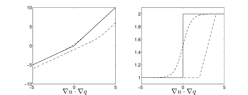
Figure 1. The functions $\mathfrak{h}$ (solid line), $\mathfrak{h}_{\delta}$ (dashed line), $\mathfrak{h}_{Tikhonov}$ (dash-dotted line) to the left and their derivatives to the right.

Another way to describe the simple regularization (12) is to see what kind of penalty on the objective function it corresponds to. We note that the regularized Hamiltionian system can be written as

$$\int_{0}^{T}\bigg{(}\int_{\Omega}-u_{t}v-\mathfrak{h}_{\delta}^{\prime}(\nabla u\cdot\nabla q)\nabla u\cdot\nabla v\ \mathrm{d}x+\int_{\partial\Omega}jv\ \mathrm{d}s\bigg{)}\ \mathrm{d}t =0, \forall v\in V,$$

$$\int_{0}^{T}\bigg{(}\int_{\Omega}q_{t}v-\mathfrak{h}_{\delta}^{\prime}(\nabla u\cdot\nabla q)\nabla q\cdot\nabla v\ \mathrm{d}x+\int_{\partial\Omega}2(u-u^{*})v\ \mathrm{d}s\bigg{)}\ \mathrm{d}t =0, \forall v\in V,$$

or by a redefinition of $\sigma$

(14) $$\int_{0}^{T}\bigg{(}\int_{\Omega}-u_{t}v-\sigma\nabla u\cdot\nabla v\ \mathrm{d}x+\int_{\partial\Omega}jv\ \mathrm{d}s\bigg{)}\ \mathrm{d}t =0, \forall v\in V,$$

$$\int_{0}^{T}\bigg{(}\int_{\Omega}q_{t}v-\sigma\nabla q\cdot\nabla v\ \mathrm{d}x+\int_{\partial\Omega}2(u-u^{*})v\ \mathrm{d}s\bigg{)}\ \mathrm{d}t =0, \forall v\in V,$$

$$\int_{0}^{T}\int_{\Omega}\Big{(}\sigma-\mathfrak{h}_{\delta}^{\prime}(\nabla u\cdot\nabla q)\Big{)}v\ \mathrm{d}x\ \mathrm{d}t =0, \forall v\in W,$$

where $\sigma:[0,T]\times\Omega\to W$ for some Hilbert space $W$. Let $\mathfrak{H}$ be the primitive function of the inverse function of $\mathfrak{h}_{\delta}^{\prime}$ i.e.

$$\mathfrak{H}(\sigma):=\frac{\delta}{2\hat{\sigma}}\bigg{(}(\sigma-\sigma_{-})\ln\Big{(}\frac{\sigma-\sigma_{-}}{\hat{\sigma}}\Big{)}+(\sigma_{+}-\sigma)\ln\Big{(}\frac{\sigma_{+}-\sigma}{\hat{\sigma}}\Big{)}\bigg{)},$$

then it is evident that (14) can be seen as the first order optimality conditions for the problem to minimize

$$\int_{0}^{T}\int_{\partial\Omega}(u-u^{*})^{2}\ \mathrm{d}s\ \mathrm{d}t+\int_{0}^{T}\int_{\Omega}\mathfrak{H}(\sigma)\ \mathrm{d}x\ \mathrm{d}t,$$

under the constraint (7). In Figure 2 the function $\mathfrak{H}(\sigma)$ is compared with a Tikhonov regularization of the form $\delta(\sigma-\bar{\sigma})^{2}$.

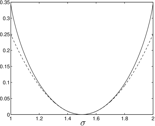
Figure 2. The function $\mathfrak{H}(\sigma)$ (solid line) compared to the $L^{2}$ penalty function $\delta(\sigma-\bar{\sigma})^{2}$ (dashed line) for $\delta=1$, $\sigma_{-}=1$ and $\sigma_{+}=2$.

It is often beneficial to prevent spacial oscillations of the coefficient by adding a penalty on the $L^{2}$-norm of the gradient of the coefficient, i.e. $\epsilon\|\nabla\sigma\|_{L^{2}(\Omega\times(0,T))}^{2}$, for $\epsilon>0$, to the objective function (8). For such a penalty the minimization in the corresponding Hamiltonian

(15) $$H(u,q,t):=\min_{\sigma:\Omega\to[\sigma_{-},\sigma_{+}]}\int_{\partial\Omega}(u-u^{*})^{2}\ \mathrm{d}s+\int_{\Omega}\mathrm{div}(\sigma\nabla u)q+\epsilon|\nabla\sigma|^{2}\ \mathrm{d}x,$$

can not be done explicitly, and instead taking the first variation in $\sigma$ would give the system

$$u_{t} =\mathrm{div}\big{(}\sigma\nabla u\big{)},$$

$$-q_{t} =\mathrm{div}\big{(}\sigma\nabla q\big{)},$$

$$2\epsilon\Delta\sigma =-\nabla u\cdot\nabla q,$$

$$\sigma \in[\sigma_{-},\sigma_{+}].$$

which corresponds to the usual first order optimality conditions for the Lagrangian. How to treat different penalties on the control in an optimal control setting is discussed in Section 3.4.

3.3. Time Independent Control

To study the case when the control $\sigma$ is independent of time we first assume that it not only is independent of time but also depends on an auxilliary variable $z$, i.e. $\sigma:\bar{\Omega}\times[0,\tilde{T}]\to[\sigma_{-},\sigma_{+}]$, $\sigma=\sigma(x,z)$. For a moment we also assume that $u:\bar{\Omega}\times[0,T]\times[0,\tilde{T}]\to V$, $u=u(x,t,z)$, but with the same measurements as in (8). If we treat $z$ as the time and $t$ as a spacial variable we can define the optimal control problem

(16) $$\min_{\sigma:\bar{\Omega}\times[0,\tilde{T}]\to[\sigma_{-},\sigma_{+}]}\frac{1}{\tilde{T}}\int_{0}^{\tilde{T}}\int_{0}^{T}\int_{\partial\Omega}(u-u^{*})^{2}\ \mathrm{d}s\ \mathrm{d}t\ \mathrm{d}z,$$

where the state $u$ satisfies the partial differential equation

(17) $$u_{z} =\frac{1}{\tilde{T}}\Big{(}\mathrm{div}(\sigma\nabla u)-u_{t}\Big{)}, \text{ in }\Omega\times(0,T)\times(0,\tilde{T}],$$

$$\sigma\nabla u\cdot\bf{n} =j, \text{ on }\partial\Omega\times(0,T)\times(0,\tilde{T}],$$

$$u =0, \text{ on }\bar{\Omega}\times\{t=0\}\times(0,\tilde{T}],$$

$$u =u_{0}, \text{ on }\bar{\Omega}\times(0,T)\times\{z=0\}.$$

for some arbitrary initial condition $u(x,t,0)=u_{0}$.

The Hamiltonian for (16), (17) is

(18) $${H}(u,q,z):= \min_{\sigma:\Omega\to[\sigma_{-},\sigma_{+}]}\frac{1}{\tilde{T}}\int_{0}^{T}\int_{\partial\Omega}(u-u^{*})^{2}\ \mathrm{d}s\ \mathrm{d}t$$

$$+\frac{1}{\tilde{T}}\int_{0}^{T}\int_{\Omega}\Big{(}\mathrm{div}(\sigma\nabla u)-u_{t}\Big{)}q\ \mathrm{d}x\ \mathrm{d}t$$

$$= \frac{1}{\tilde{T}}\int_{0}^{T}\int_{\partial\Omega}(u-u^{*})^{2}+jq\ \mathrm{d}s\ \mathrm{d}t-\frac{1}{\tilde{T}}\int_{0}^{T}\int_{\Omega}u_{t}q\ \mathrm{d}x\ \mathrm{d}t$$

$$-\frac{1}{\tilde{T}}\int_{\Omega}\underbrace{\max_{\sigma\in[\sigma_{-},\sigma_{+}]}\bigg{\{}\sigma\int_{0}^{T}\nabla u\cdot\nabla q\ \mathrm{d}t\bigg{\}}}_{\mathfrak{h}\big{(}\int_{0}^{T}\nabla u\cdot\nabla q\ \mathrm{d}t\big{)}}\ \mathrm{d}x,$$

and the Hamiltonian system is given by

(19) $$u_{z} =\frac{1}{\tilde{T}}\Big{(}\mathrm{div}(\mathfrak{h}^{\prime}\nabla u)-u_{t}\Big{)}, \text{ in }\Omega\times(0,T)\times(0,\tilde{T}],$$

$$\mathfrak{h}^{\prime}\nabla u\cdot\bf{n} =j, \text{ on }\partial\Omega\times(0,T)\times(0,\tilde{T}],$$

$$u =0, \text{ on }\bar{\Omega}\times\{t=0\}\times(0,\tilde{T}],$$

$$u =u_{0}, \text{ on }\bar{\Omega}\times(0,T)\times\{z=0\},$$

$$-q_{z} =\frac{1}{\tilde{T}}\Big{(}\mathrm{div}(\mathfrak{h}^{\prime}\nabla q)+q_{t}\Big{)}, \text{ in }\Omega\times(0,T)\times(0,\tilde{T}],$$

$$\mathfrak{h}^{\prime}\nabla q\cdot\bf{n} =2(u-u^{*}), \text{ on }\partial\Omega\times(0,T)\times(0,\tilde{T}],$$

$$q =0, \text{ on }\bar{\Omega}\times\{t=T\}\times(0,\tilde{T}],$$

$$q =0, \text{ on }\bar{\Omega}\times(0,T)\times\{z=\tilde{T}\}.$$

Under the assumption that the solutions $u$ and $q$ in (19) are asymptotically stationary as $\tilde{T}\to\infty$, the Hamiltonian system for the problem (7), (8), with a time-independent control, is given by (10) and

(20) $$\tilde{\sigma}:=\mathfrak{h}^{\prime}\bigg{(}\int_{0}^{T}\nabla u\cdot\nabla q\ \mathrm{d}t\bigg{)}.$$

Similarly, the case of a space independent coefficient $\sigma=\sigma(t)$ will lead to

$$\tilde{\sigma}:=\mathfrak{h}^{\prime}\bigg{(}\frac{1}{|\Omega|}\int_{\Omega}\nabla u\cdot\nabla q\ \mathrm{d}x\bigg{)},$$

and for the case where $\sigma$ is constant

$$\tilde{\sigma}:=\mathfrak{h}^{\prime}\bigg{(}\frac{1}{|\Omega|}\int_{0}^{T}\int_{\Omega}\nabla u\cdot\nabla q\ \mathrm{d}x\ \mathrm{d}t\bigg{)}.$$

3.4. Penalty on the Control

If we want to reconstruct a time independent control it can be beneficial to put a penalty on $\sigma_{t}$, i.e. we want to minimize the objective functional

(21) $$F(u,\sigma_{t}):=\int_{0}^{T}\int_{\partial\Omega}(u-u^{*})^{2}\ \mathrm{d}s\ \mathrm{d}t+\varepsilon\int_{0}^{T}\int_{\Omega}\sigma_{t}^{2}\ \mathrm{d}x\ \mathrm{d}t,$$

under the usual constraint (7). To do this the optimal control problem has to be reformulated such that $\sigma$ is a state variable and the control is defined as $z:=\sigma_{t}(x,t)$, $z:\bar{\Omega}\times[0,T]\to[z_{-},z_{+}]$. The optimal control problem is thus to find a control $z$ and state variables $u$ and $\sigma$ such that $F(u,z)$ is minimized and the system

$$u_{t} =\mathrm{div}(\sigma\nabla u), \text{ in }\Omega\times(0,T],$$

$$\sigma_{t} =z \text{ in }\Omega\times(0,T],$$

$$\sigma\nabla u\cdot\bf{n} =j, \text{ on }\partial\Omega\times(0,T],$$

$$u =0, \text{ on }\bar{\Omega}\times\{t=0\},$$

$$\sigma =\sigma_{0}>0, \text{ on }\bar{\Omega}\times\{t=0\}.$$

is satisfied. The Hamiltonian becomes

$${H}(u,q,\sigma,\lambda,t):= \min_{z:\Omega\to[z_{-},z_{+}]}\int_{\partial\Omega}(u-u^{*})^{2}\ \mathrm{d}s+\int_{\Omega}\mathrm{div}(\sigma\nabla u)q+z\lambda+\varepsilon z^{2}\ \mathrm{d}x$$

$$= \int_{\partial\Omega}(u-u^{*})^{2}+jq\ \mathrm{d}s-\int_{\Omega}\sigma\nabla u\cdot\nabla q\ \mathrm{d}x$$

$$+\int_{\Omega}\underbrace{\min_{z:\Omega\to[z_{-},z_{+}]}\{z(\varepsilon z+\lambda)\}}_{\mathfrak{h}(\lambda)}\ \mathrm{d}x,$$

and the corresponding Hamiltonian system is

$$u_{t} =\mathrm{div}\big{(}\sigma\nabla u\big{)}, \text{ in }\Omega\times(0,T],$$

$$\sigma_{t} =\mathfrak{h}^{\prime}(\lambda) \text{ in }\Omega\times(0,T],$$

$$\sigma\nabla u\cdot\bf{n} =j, \text{ on }\partial\Omega\times(0,T],$$

$$u =0, \text{ on }\bar{\Omega}\times\{t=0\},$$

$$\sigma =\sigma_{0}>0, \text{ on }\bar{\Omega}\times\{t=0\}.$$

$$-q_{t} =\mathrm{div}\big{(}\sigma\nabla q\big{)}, \text{ in }\Omega\times(0,T],$$

$$-\lambda_{t} =-\nabla u\cdot\nabla q \text{ in }\Omega\times(0,T],$$

$$\sigma\nabla q\cdot\bf{n} =2(u-u^{*}), \text{ on }\partial\Omega\times(0,T],$$

$$q =0, \text{ on }\Omega\times\{t=T\},$$

$$\lambda =0, \text{ on }\Omega\times\{t=T\},$$

which is equivalent to (10) with

$$\tilde{\sigma}:=\sigma_{0}+\int_{0}^{t}\mathfrak{h}^{\prime}\bigg{(}\int_{y}^{T}-(\nabla u\cdot\nabla q)(x,z)\ \mathrm{d}z\bigg{)}\ \mathrm{d}y.$$

Note, since we no longer have a constraint $\sigma>0$, the bound $z_{-}$ has to be carefully chosen to ensure well-posedness of the forward problem.

In a similar fashion as for penalizing temporal variations of the control it is also possible to penalize spacial variations, as was briefly mentioned in Section 3.2, where the objective was to minimize $F(u,|\nabla\sigma|)$ under the constraint (7), which leads to the Hamiltonian (15). To be able to explicitly find the minimum in the Hamiltonian we once again let $\sigma$ act as a state variable, introduce the control $z$ and the dynamics

(22) $$\sigma_{t} =\frac{z-|\nabla\sigma|^{2}}{\gamma}, \text{ in }\Omega\times(0,T],$$

$$\sigma =\sigma_{0}>0, \text{ in }\Omega\times\{t=0\},$$

for $\gamma>0$. The slightly perturbed control problem is now to minimize the objective function $F(u,z)$ such that (7) and (22) holds, which leads to the Hamiltonian

$${H}(u,q,\sigma,\lambda,t):= \min_{z:\Omega\to[z_{-},z_{+}]}\int_{\partial\Omega}(u-u^{*})^{2}\ \mathrm{d}s+\int_{\Omega}\mathrm{div}(\sigma\nabla u)q+\lambda\frac{z-|\nabla\sigma|^{2}}{\gamma}+\varepsilon z\ \mathrm{d}x$$

$$= \int_{\partial\Omega}(u-u^{*})^{2}+jq\ \mathrm{d}s-\int_{\Omega}\sigma\nabla u\cdot\nabla q+\lambda\frac{|\nabla\sigma|^{2}}{\gamma}\ \mathrm{d}x$$

$$+\int_{\Omega}\underbrace{\min_{z:\Omega\to[z_{-},z_{+}]}\{z(\varepsilon+\frac{\lambda}{\gamma})\}}_{\mathfrak{h}(\lambda)}\ \mathrm{d}x,$$

and the Hamiltonian system

$$u_{t} =\mathrm{div}\big{(}\sigma\nabla u\big{)},$$

$$\sigma_{t} =\mathfrak{h}^{\prime}(\lambda)-\frac{|\nabla\sigma|^{2}}{\gamma},$$

$$-q_{t} =\mathrm{div}\big{(}\sigma\nabla q\big{)},$$

$$-\lambda_{t} =\nabla u\cdot\nabla q-2\lambda\frac{\Delta\sigma}{\gamma}.$$

3.5. Numerical Approximation and Symplectic Methods

Let $\bar{V}\subset V:=H^{1}(\Omega)$ be the finite element subspace of piecewise linear functions defined on a triangulation of $\Omega$, which implies that our optimal control problems in the previous sections are approximated by optimal control problems for ordinary differential equations. We also let the functions $\mathfrak{h}_{\delta}$,$H^{\delta}$ and $h_{\delta}$ denote the regularized counterparts to $\mathfrak{h}$,$H$ and $h$. The regularized version of $\mathfrak{h}$ is given by (12) from which the definition of $H^{\delta}$ follows. The regularized function $h_{\delta}$ can be derived from $H^{\delta}$ by $h_{\delta}:=H^{\delta}-\langle\lambda,H_{\lambda}^{\delta}\rangle$ and a regularized version of $f$ can be defined as $f_{\delta}:=H_{\lambda}^{\delta}$.

Now, introduce the uniform partition $\{t_{i}=ki\}_{i=0}^{N}$, $k=T/N$ of the time interval $[0,T]$, and the corresponding finite element approximations at each time step $\varphi_{n}:=\varphi(t_{n}),\lambda_{n}:=\lambda(t_{n})$. Also define a discrete regularized version $\bar{U}:\bar{V}\times[0,T]\to\mathbb{R}$ of the value function (2),

$$\bar{U}(\phi,t_{m}):=\min_{\varphi_{m}=\phi}\bigg{\{}g(\varphi_{N})+k\sum_{n=m}^{N-1}h_{\delta}(\varphi_{n},\lambda_{n+1})\bigg{\}},$$

where $\varphi_{n}$ and $\lambda_{n}$ satisfy a symplectic scheme, e.g. the symplectic forward Euler method

(23) $$\varphi_{n+1}-\varphi_{n} =k{H}_{\lambda}^{\delta}(\varphi_{n},\lambda_{n+1}), \text{ for }n=m,\ldots,N-1\text{ given }\varphi_{m}=\phi,$$

$$\lambda_{n}-\lambda_{n+1} =k{H}_{\varphi}^{\delta}(\varphi_{n},\lambda_{n+1}), \text{ for }n=m,\ldots,N-1\text{ given }\lambda_{N}=g_{\varphi}(\varphi_{N}).$$

Symplecticity here means that $\bar{U}_{\varphi}(\varphi_{n},t_{n})=\lambda_{n}$, i.e. the gradient of the discrete value function coincides with the discrete dual $\lambda_{n}$, and given that $|H-H^{\delta}|=\mathcal{O}(\delta)$ it can be shown that for symplectic one-step schemes

$$\bigg{|}U(\varphi_{0},t_{0})-g(\varphi_{N})-k\sum_{n=m}^{N-1}h_{\delta}(\varphi_{n},\lambda_{n+1})\bigg{|}=\mathcal{O}(k),$$

for $\delta\sim k$, see [15]. It is thus essential to use a symplectic time discretization of the regularized Hamiltonian system

$$\varphi_{t} ={H}_{\lambda}^{\delta}(\varphi,\lambda),$$

$$\lambda_{t} =-{H}_{\varphi}^{\delta}(\varphi,\lambda),$$

in order to have convergence in the value function.

Some examples of other symplectic schemes are the the backward Euler method

(24) $$\varphi_{n+1}-\varphi_{n} =k{H}_{\lambda}^{\delta}(\varphi_{n+1},\lambda_{n}), \text{ for }n=0,\ldots,N-1\text{ given }\varphi_{0},$$

$$\lambda_{n}-\lambda_{n+1} =k{H}_{\varphi}^{\delta}(\varphi_{n+1},\lambda_{n}), \text{ for }n=0,\ldots,N-1\text{ given }\lambda_{N},$$

and the implicit midpoint method

(25) $$\varphi_{n+1}-\varphi_{n} =k{H}_{\lambda}^{\delta}\bigg{(}\frac{\varphi_{n}+\varphi_{n+1}}{2},\frac{\lambda_{n}+\lambda_{n+1}}{2}\bigg{)}, \text{ for }n=0,\ldots,N-1\text{ given }\varphi_{0},$$

$$\lambda_{n}-\lambda_{n+1} =k{H}_{\varphi}^{\delta}\bigg{(}\frac{\varphi_{n}+\varphi_{n+1}}{2},\frac{\lambda_{n}+\lambda_{n+1}}{2}\bigg{)}, \text{ for }n=0,\ldots,N-1\text{ given }\lambda_{N}.$$

See [12] for a thorough description of symplectic methods.

3.6. The Newton Method

To solve the coupled nonlinear symplectic schemes (23)-(25) above, it is tempting to propose fix-point schemes that partly removes the coupling between the forward and bacward equation, e.g. by iterating separately in $\varphi$ and $\lambda$. Such methods has the advantage that existing partial differential equation solvers can be used to efficiently solve the forward and backward problems in each iteration, but the disadvantage is that the convergence to an optimal solution tends to be slow, and also dependent on the discretisation. A more suitable strategy is to use information of the Hessian of $H^{\delta}$; e.g. Quasi-Newton methods, or since the Hessian in our case can be found explicitly and is sparse, the Newton method itself.

For the Hamiltonian system (10) with $\tilde{\sigma}:=\mathfrak{h}_{\delta}^{\prime}$ given by (12) the symplectic backward Euler can be written as

$$F_{n}(w)=0,\quad G_{n}(w)=0,\quad n=0,\ldots,N-1,\quad\forall w\in\bar{V}$$

where

(26) $$F_{n}(w):= \int_{\Omega}(u_{n+1}-u_{n})w+k\mathfrak{h}_{\delta}^{\prime}(\nabla u_{n+1}\cdot\nabla q_{n})\nabla u_{n+1}\cdot\nabla w\ \mathrm{d}x$$

$$-\int_{\partial\Omega}kj_{n+1}w\ \mathrm{d}s,$$

$$G_{n}(w):= \int_{\Omega}(q_{n}-q_{n+1})w+k\mathfrak{h}_{\delta}^{\prime}(\nabla u_{n+1}\cdot\nabla q_{n})\nabla q_{n}\cdot\nabla w\ \mathrm{d}x$$

$$-\int_{\partial\Omega}2k(u_{n+1}-u^{*}_{n+1})w\ \mathrm{d}s,$$

and $u_{0}=q_{N}=0$. Given an initial guess $u[0]$, $q[0]$ the (damped) Newton method yields that

$$u[i+1]=u[i]-\alpha\hat{u},$$

$$q[i+1]=q[i]-\alpha\hat{q},$$

where $\alpha\in(0,1]$ and, for each iteration, the updates $\hat{u}$ and $\hat{q}$ solve a linear system of the form

(27) $$\left(\begin{array}[]{cc}K_{11}&K_{12}\\ K_{21}&K_{11}^{T}\end{array}\right)\left(\begin{array}[]{c}\hat{u}\\ \hat{q}\end{array}\right)=\left(\begin{array}[]{c}f\\ g\end{array}\right),$$

where

$$\hat{u}= \left(\begin{array}[]{ccccc}\hat{u}_{1}&\ldots&\hat{u}_{N}\end{array}\right)^{T}, \hat{q}= \left(\begin{array}[]{ccccc}\hat{q}_{0}&\ldots&\hat{q}_{N-1}\end{array}\right)^{T},$$

$$f= \left(\begin{array}[]{ccccc}F_{0}&\ldots&F_{N-1}\end{array}\right)^{T}, g= \left(\begin{array}[]{ccccc}G_{0}&\ldots&G_{N-1}\end{array}\right)^{T}.$$

The matrix $K_{11}$ is a bi-diagonal block matrix with $M+S_{i}$ for $i=0,\ldots,N-1$ on the diagonal and $-M$ on the sub-diagonal, where $M$ denotes the mass matrix

$$\int_{\Omega}w\bar{w}\ \mathrm{d}x,$$

and

$$S_{n}:= \int_{\Omega}k\mathfrak{h}_{\delta}^{\prime\prime}(\nabla u_{n+1}\cdot\nabla q_{n})\nabla q_{n}\cdot\nabla w\ \nabla u_{n+1}\cdot\nabla\bar{w}\ \mathrm{d}x$$

$$+\int_{\Omega}k\mathfrak{h}_{\delta}^{\prime}(\nabla u_{n+1}\cdot\nabla q_{n})\nabla w\cdot\nabla\bar{w}\ \mathrm{d}x.$$

for $w,\bar{w}\in\bar{V}$. The matrices $K_{12}$, $K_{21}$ are symmetric block-diagonal matrices with

$$\int_{\Omega}k\mathfrak{h}_{\delta}^{\prime\prime}(\nabla u_{n+1}\cdot\nabla q_{n})\nabla u_{n+1}\cdot\nabla w\ \nabla u_{n+1}\cdot\nabla\bar{w}\ \mathrm{d}x,$$

and

$$\int_{\Omega}k\mathfrak{h}_{\delta}^{\prime\prime}(\nabla u_{n+1}\cdot\nabla q_{n})\nabla q_{n}\cdot\nabla w\ \nabla q_{n}\cdot\nabla\bar{w}\ \mathrm{d}x-\int_{\partial\Omega}2k\bar{w}w\ \mathrm{d}s,$$

for $n=0,\ldots,N-1$ on the the diagonals, respectively.

If we repartition the block $2\times 2$ linear system (27) to

(28) $$\left(\begin{array}[]{cc}K_{21}&K_{11}^{T}\\ K_{11}&K_{12}\end{array}\right)\left(\begin{array}[]{c}\hat{u}\\ \hat{q}\end{array}\right)=\left(\begin{array}[]{c}g\\ f\end{array}\right),$$

we see that it is a generalized saddle point system [4] with symmetric matrices $K_{21},K_{12}$, and $K_{11}^{T}\neq 0$, $K_{21}\neq 0$. However, unlike saddle point problems arising from e.g. the steady-state Navier-Stokes equations or from the Karush-Kuhn-Tucker optimality conditions for equality constrained minimization problems, both $K_{12}$ and $K_{21}$ may here be indefinite and singular.

Since (27) and (28) are increasingly ill-conditioned with respect to reduction in mesh size, step size and regularization, the success of iterative algorithms like Krylov sub-space methods will depend heavily on the choice of preconditioner. Standard algebraic preconditioners like incomplete LU-factorization are often unsuitable for saddle-point problems due to the indefiniteness and lack of diagonal dominance, so the preconditioner must be tailored for the specific problem at hand. One popular approach for PDE-constrained optimization problems is to base the preconditioner on the solution from a reduced approximated problem where the Schur complement is replaced by an approximation e.g. by quasi-newton methods, see [5].

In our case we use the GMRES method to solve the non-symmetric system (27) and base our preconditioner on the approximate solution of a simple blockwise Gauss-Seidel method i.e. to start with a guess $\hat{q}^{0}$ and iteratively solve

(29) $$K_{11}\hat{u}^{i+1} =f-K_{12}\hat{q}^{i},$$

$$K_{11}^{T}\hat{q}^{i+1} =g-K_{21}\hat{u}^{i+1},$$

which works well for large regularizations i.e. when $\mathfrak{h}_{\delta}^{\prime\prime}$ is small and the diagonal blocks of (27) are dominant. Also, each iteration with this method only requires one forward and one backward solve in time of a modified heat equation so the computational work for one iteration is concentrated to solving $N-1$ smaller systems with system matrices $(M+S_{i})$. In practice, the Gauss-Seidel method will break down for small regularizations but for our problems (and discretizations) only one iteration with (29) turns out to be a fairly good approximation to use as preconditioner. Note that for $\hat{q}^{0}=0$, one Gauss-Seidel iteration is the same as solving (27) with the approximation $K_{12}=0$.

Another more elaborate idea is to use a preconditioner based on the solution of an approximated Schur complement system

$$\left(\begin{array}[]{cc}K_{11}&K_{12}\\ 0&S\end{array}\right)\left(\begin{array}[]{c}\hat{u}\\ \hat{q}\end{array}\right)=\left(\begin{array}[]{c}g\\ f-K_{12}K_{11}^{-1}g\end{array}\right),$$

where $S$ is an approximation of the Schur complement

$$K_{11}^{T}-K_{21}K_{11}^{-1}K_{12}.$$

which essentially is to find a good approximation of the lower triangular block matrix $K_{11}^{-1}$.

Although solution algorithms for saddle point systems on the symmetric form (28) are extensively treated in the litterature, see [4] for an overview, we here favour the non-symmetric form (27), since a Schur complement reduction of (28) means to find an approximation to the Schur complement

$$K_{12}-K_{11}K_{21}^{-1}K_{11}^{T},$$

which since $K_{21}$ here can be singular, is unavailable. One way around this obstacle is to rewrite (28) by e.g. the augmented Lagrangian method which leads to a symmetric invertible Schur complement but where the physical meaning of the original system, on PDE level, is partially lost.

If a direct solver is used for the Newton system it is appropriate to reorder (27) such that the solution vector and right hand side contains time steps in increasing order, which leads to a banded Jacobian with band-width of the same order as the number of spacial degrees of freedom.

Our computations were implemented MATLAB (for the one dimensional examples), and in DOLFIN [13], the C++/Python interface of the finite element solver environment FEniCS [11] (for the two dimensional examples). Piecewise linear basis functions were used for the finite element subspace $\bar{V}$, and in all examples the solution $u,q$ was first calculated for a large regularization which was succesively reduced such that the solution from the previous regularization served as starting guess for a smaller regularization.

For the two dimensional examples the sadde-point system (27) was solved with the PETSc implementation of GMRES (used by DOLFIN) with preconditioning based on the solution from one iteration of blockwise Gauss-Seidel method. For the one dimensional examples a direct solver was used. The number of iterations for GMRES with the Gauss-Seidel preconditioner seems to be relatively insensitive with respect to temporal and spacial discretization but still highly sensitive to the regularization in our examples.

To give a time independent approximation $\sigma(x)$ of the time dependent control $\sigma(x,t)$, approximated by $\tilde{\sigma}:=\mathfrak{h}_{\delta}^{\prime}(\nabla u\cdot\nabla q)$ where $u,q$ are solutions to the Hamiltonian system (10), three different types of averaging were tested as post-processing:

1. Let the time independent control be defined by the Hamiltonian (18), i.e.

   (30) $$\sigma:=\mathfrak{h}_{\delta}^{\prime}\bigg{(}\int_{0}^{T}\nabla u\cdot\nabla q\ \mathrm{d}t\bigg{)}.$$

2. Let the time independent control be the average of the time dependent control, i.e.

   (31) $$\sigma:=\frac{1}{T}\int_{0}^{T}\mathfrak{h}_{\delta}^{\prime}(\nabla u\cdot\nabla q)\ \mathrm{d}t.$$

3. Let the time independent control be the weighted average

   (32) $$\sigma:=\frac{\int_{0}^{T}\mathfrak{h}_{\delta}^{\prime}(\nabla u\cdot\nabla q)|\nabla u\cdot\nabla q|\ \mathrm{d}t}{\int_{0}^{T}|\nabla u\cdot\nabla q|\ \mathrm{d}t},$$

   of the time dependent control $\mathfrak{h}_{\delta}^{\prime}(\nabla u\cdot\nabla q)$.

The weighted average turned out to be the most successful aproximation and can be explained by first extending the Hamiltonian (9) to also depend on the artifical variable $z$ as in Section 3.3

$$H(u,q,z):= \frac{1}{\tilde{T}}\int_{0}^{T}\int_{\partial\Omega}(u-u^{*})^{2}+jq\ \mathrm{d}s\ \mathrm{d}t-\frac{1}{\tilde{T}}\int_{0}^{T}\int_{\Omega}u_{t}q\ \mathrm{d}x\ \mathrm{d}t$$

$$-\frac{1}{\tilde{T}}\int_{\Omega}\int_{0}^{T}\mathfrak{h}^{\prime}(\nabla u\cdot\nabla q)\nabla u\cdot\nabla q\ \mathrm{d}t\ \mathrm{d}x,$$

where $\mathfrak{h}^{\prime}(\nabla u\cdot\nabla q)\nabla u\cdot\nabla q=\mathfrak{h}(\nabla u\cdot\nabla q)$ by definition. For the problem with a time independent control we now seek an approximation of the Hamiltonian (18) of the form

$$\bar{H}(u,q,z):= \frac{1}{\tilde{T}}\int_{0}^{T}\int_{\partial\Omega}(u-u^{*})^{2}+jq\ \mathrm{d}s\ \mathrm{d}t-\frac{1}{\tilde{T}}\int_{0}^{T}\int_{\Omega}u_{t}q\ \mathrm{d}x\ \mathrm{d}t$$

$$-\frac{1}{\tilde{T}}\int_{\Omega}f(\nabla u\cdot\nabla q)\int_{0}^{T}\nabla u\cdot\nabla q\ \mathrm{d}t\ \mathrm{d}x,$$

that best approximates $H$, i.e.

$$f(\nabla u\cdot\nabla q):=\frac{\int_{0}^{T}\mathfrak{h}^{\prime}(\nabla u\cdot\nabla q)\nabla u\cdot\nabla q\ \mathrm{d}t}{\int_{0}^{T}\nabla u\cdot\nabla q\ \mathrm{d}t}.$$

In Figure 3, one dimensional reconstructions from three sets of simulated data $u^{*}$, generated from a time independent conductivity $\sigma_{true}$, are compared:

1. Data calculated with the same discretization as $u$ and $q$.

2. Different discretisations used for data and solutions.

3. Different discretisations used for data and solutions and with noise in the data $u^{*}$.

The last set is the most realistic one since for true experimental data of $u^{*}$ it is inevitable to not only have measurement noise but also a systematic error from the numerical method. To simulate noise the discrete solution $u^{*}$ was multiplied componentwise by independent standard normal distributed stochastic variables $\varepsilon_{ij}$ according to $u^{*}(x_{i},t_{j})(1+\eta\epsilon_{ij})$, where $\eta$ denotes the percentage of noise. It is notable that the systematic error from using different meshes can have a much bigger effect on the solutions than additional noise, which can be observed from the dual solution $q$ in Figure 3.

In Figure 4 the time independent post-processing of the time dependent reconstruction can be found. It is here evident that the weighted average (32) performs better than (31), but since the reconstruction is highly dependent on the given boundary condition, see Figure 5 for comparison, there are situations where the different post-processing techniques perform equally well. It would of course be optimal to use the knowledge that $\sigma_{true}$ is independent of time in the calculations, i.e. to use the Newtion system for (10) with time independent-control (20). This would however lead to a dense Jacobian.

Note that in the examples the limits $\sigma_{-},\sigma_{+}$ were chosen to be the biggest and smallest values of $\sigma_{true}$. In our experience the Pontryagin method is not well suited for reconstruction of values between $\sigma_{-}$ and $\sigma_{+}$ if there is noise or other measurement errors present in data.

Figure 6 shows two-dimensional reconstructions of two different time independent conductivities. Unlike the one-dimensional example the quality of the reconstruction here deteriorates quickly as the distance to the measurement locations is increased.

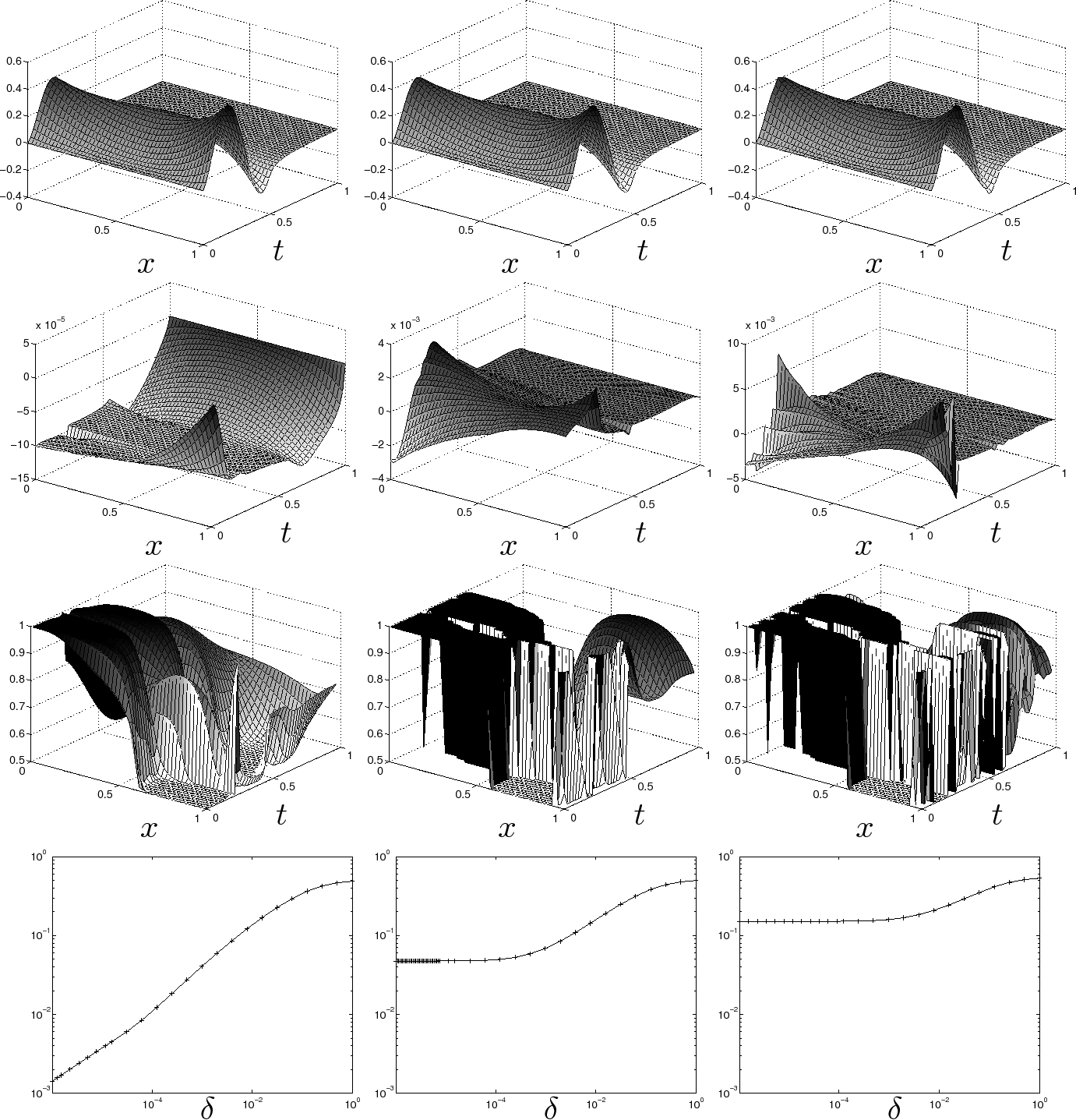
Figure 3. 1D reconstruction of $\sigma_{true}=0.75-0.5\tanh(20x-10)$ with $\delta=10^{-6}$, $\sigma_{-}=0.5$, $\sigma_{+}=1$, measurements on both boundaries and Neumann boundary condition $\sigma u_{x}(0,t)=-\sigma u_{x}(1,t)=\sin(4t)$ for $t<0.5$ and $0$ elsewhere. The plot shows, from top to bottom, $u$, $q$, $\mathfrak{h}_{\delta}^{\prime}$ and the objective function $\|u-u^{*}\|_{L^{2}(\partial\Omega\times[0,T])}$. In all cases $u,q$ was calculated with 50 steps in space and time. In the left column, the data $u^{*}$ was generated by solving the heat equation with 50 steps in time and space and conductivity $\sigma_{true}$, while 200 steps in time and space was used in the middle and right columns. In the right column 10% noise was also added to $u^{*}$.

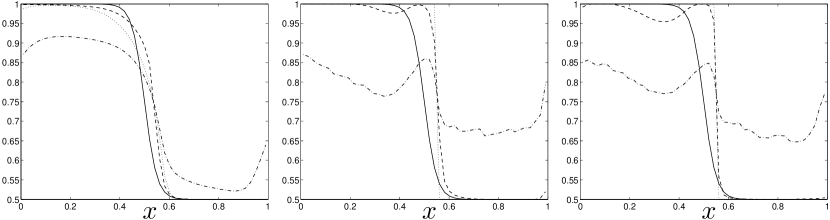
Figure 4. The time independent post-processed conductivity for the 1D reconstructions in Figure 3. The true control $\sigma_{true}$ is indicated by a solid line and the averaged controls (30), (31) and (32) are indicated by dotted, dash-dotted and dashed lines, respectively.

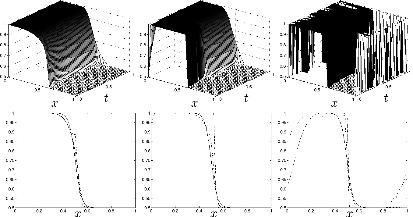
Figure 5. 1D reconstruction with data as in Figure 3 and 4 but with Neumann boundary condition $\sigma u_{x}(0,t)=-\sigma u_{x}(1,t)=1$.

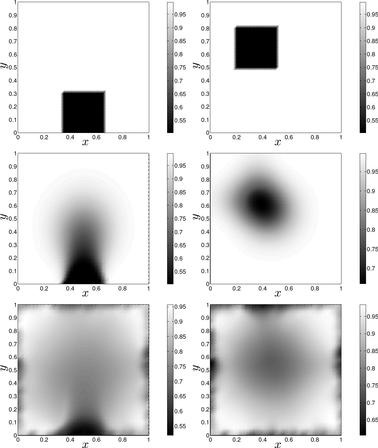
Figure 6. 2D reconstruction on the unit square with final time $T=1$ and Neumann boundary condition $\sigma\frac{\partial u}{\partial n}=1$ on $\partial\Omega\times[0,T]$. The data $u^{*}$ was simulated by solving the forward equation on a quasi-uniform mesh with 13000 triangles and 80 time steps while the inverse problem was solved on a uniform mesh with 3200 triangles and 40 time steps. Measurements from the whole boundary were used. Top: True conductivity $\sigma_{true}$. Middle: Reconstructed condictivity for $\delta\approx 0.002$ using the weighted average (32). Bottom: As in middle but for $\delta\approx 0.05$ and with 5% noise in the measurements.

4. Reconstruction from the Wave Equation

In this section the goal is to determine the wave speed for a scalar acoustic wave equation: Given measured data $u^{*}$, find the state $u:\bar{\Omega}\times[0,T]\to V$, $u=u(x,t)$ and a control e.g. $\sigma:\bar{\Omega}\times[0,T]\to[\sigma_{-},\sigma_{+}]$, $\sigma=\sigma(x,t)$ where $0<\sigma_{-}<\sigma_{+}$, that solves the partial differential equation

(33) $$u_{tt} =\mathrm{div}(\sigma\nabla u), \text{ in }\Omega\times(0,T],$$

$$\sigma\nabla u\cdot\bf{n} =j, \text{ on }\partial\Omega\times(0,T],$$

$$u =u_{t}=0, \text{ on }\bar{\Omega}\times\{t=0\},$$

such that the error functional

(34) $$\int_{0}^{T}\int_{\partial\Omega}(u-u^{*})^{2}\ \mathrm{d}s\ \mathrm{d}t,$$

is minimized. The control $\sigma$ is here the square of the wave speed of the medium and $u$ is the pressure deviation.

To use the framework of the previous section we note that (33) can be written as the first order system

(35) $$v_{t} =\mathrm{div}(\sigma\nabla u), \text{ in }\Omega\times(0,T],$$

$$u_{t} =v, \text{ in }\bar{\Omega}\times(0,T],$$

$$\sigma\nabla u\cdot\bf{n} =j, \text{ on }\partial\Omega\times(0,T],$$

$$u =v=0, \text{ on }\bar{\Omega}\times\{t=0\}.$$

4.1. The Hamiltonian System

As in Section 3.1 we have a Hamiltonian associated with the optimal control problem (34) and (35) which is defined by

(36) $${H} :=\min_{\sigma:\Omega\to[\sigma_{-},\sigma_{+}]}\int_{\partial\Omega}(u-u^{*})^{2}\ \mathrm{d}s+\int_{\Omega}\mathrm{div}(\sigma\nabla u)q+vp\ \mathrm{d}x$$

$$=\int_{\partial\Omega}(u-u^{*})^{2}+jq\ \mathrm{d}s+\min_{\sigma:\Omega\to[\sigma_{-},\sigma_{+}]}\int_{\Omega}-\sigma\nabla u\cdot\nabla q+vp\ \mathrm{d}x$$

$$=\int_{\partial\Omega}(u-u^{*})^{2}+jq\ \mathrm{d}s+\int_{\Omega}vp-\underbrace{\max_{\sigma\in[\sigma_{-},\sigma_{+}]}\{\sigma\nabla u\cdot\nabla q\}}_{\mathfrak{h}(\nabla u\cdot\nabla q)}\ \mathrm{d}x,$$

and the Hamiltonian system becomes

(37) $$v_{t} =\mathrm{div}\big{(}\tilde{\sigma}\nabla u\big{)}, \text{ in }\Omega\times(0,T],$$

$$u_{t} =v, \text{ in }\bar{\Omega}\times(0,T],$$

$$\tilde{\sigma}\nabla u\cdot\bf{n} =j, \text{ on }\partial\Omega\times(0,T],$$

$$u =v=0, \text{ on }\bar{\Omega}\times\{t=0\},$$

$$-p_{t} =\mathrm{div}\big{(}\tilde{\sigma}\nabla q\big{)}, \text{ in }\Omega\times(0,T],$$

$$-q_{t} =p, \text{ in }\bar{\Omega}\times(0,T],$$

$$\tilde{\sigma}\nabla q\cdot\bf{n} =2(u-u^{*}), \text{ on }\partial\Omega\times(0,T],$$

$$p =q=0, \text{ on }\Omega\times\{t=T\},$$

or equivalently

(38) $$u_{tt} =\mathrm{div}\big{(}\tilde{\sigma}\nabla u\big{)}, \text{ in }\Omega\times(0,T],$$

$$\tilde{\sigma}\nabla u\cdot\bf{n} =j, \text{ on }\partial\Omega\times(0,T],$$

$$u =u_{t}=0, \text{ on }\bar{\Omega}\times\{t=0\},$$

$$q_{tt} =\mathrm{div}\big{(}\tilde{\sigma}\nabla q\big{)}, \text{ in }\Omega\times(0,T],$$

$$\tilde{\sigma}\nabla q\cdot\bf{n} =2(u-u^{*}), \text{ on }\partial\Omega\times(0,T],$$

$$q =q_{t}=0, \text{ on }\bar{\Omega}\times\{t=T\}.$$

with

$$\tilde{\sigma}:=\mathfrak{h}^{\prime}(\nabla u\cdot\nabla q).$$

4.2. Symplecticity for the Wave Equation

As a natural case the symplectic methods discussed in 3.5, with $\varphi=(u,v)$, $\lambda=(p,q)$, can be used to solve the system (37). It is however also possible to use a time-discretization that is symmetric in time i.e.

(39) $$u_{n+1}-2u_{n}+u_{n-1} =k^{2}\mathrm{div}\big{(}\tilde{\sigma}_{n}\nabla u_{n}\big{)}, \text{ in }\Omega,$$

$$\tilde{\sigma}_{n}\nabla u_{n}\cdot\bf{n} =j_{n}, \text{ on }\partial\Omega,$$

$$u_{0} =u_{1}=0, \text{ in }\Omega,$$

$$q_{n+1}-2q_{n}+q_{n-1} =k\mathrm{div}\big{(}\tilde{\sigma}_{n}\nabla q_{n}\big{)}, \text{ in }\Omega,$$

$$\tilde{\sigma}_{n}\nabla q_{n}\cdot\bf{n} =2(u_{n}-u^{*}_{n}), \text{ on }\partial\Omega,$$

$$q_{N} =q_{N-1}=0, \text{ in }\Omega,$$

for $\tilde{\sigma}_{n}:=\mathfrak{h}^{\prime}(\nabla u_{n}\cdot\nabla q_{n})$ and $n=1,\ldots,N-1$. For a given $\tilde{\sigma}$, constant in time, this scheme is the symplectic backward Euler method for the forward wave equation for $u$, which can be written as the Hamiltonian system (35) with Hamiltonian

$${H}_{wave}(u,v):=\frac{1}{2}\int_{\Omega}|\tilde{\sigma}\nabla u|^{2}+v^{2}\ \mathrm{d}x,$$

and the symplectic forward Euler method for the backward wave equation for $q$.

To see that that the scheme (39) is symplectic for $\tilde{\sigma}_{n}:=\mathfrak{h}^{\prime}(\nabla u_{n}\cdot\nabla q_{n})$ we note that a one-step method $(\varphi_{n},\lambda_{n})\to(\varphi_{n+1},\lambda_{n+1})$ is symplectic if there exists a function ${H}(\varphi_{n},\lambda_{n+1})$ such that (23) holds, or equivalently ${H}(\varphi_{n+1},\lambda_{n})$ such that (24) holds, see Remark 4.8 in [15] or [12] for details. It thus follows that the one-step method

$$v_{n+1}-v_{n} =k\mathrm{div}\big{(}\mathfrak{h}^{\prime}(\nabla u_{n}\cdot\nabla q_{n})\nabla u_{n}\big{)},$$

$$u_{n+1}-u_{n} =kv_{n+1},$$

$$p_{n}-p_{n+1} =k\mathrm{div}\big{(}\mathfrak{h}^{\prime}(\nabla u_{n}\cdot\nabla q_{n})\nabla q_{n}\big{)},$$

$$q_{n}-q_{n+1} =kp_{n+1},$$

corresponds to the symplectic forward Euler method for the Hamiltonian

$$\tilde{H}(\underbrace{u_{n},q_{n}}_{\varphi_{n}},\underbrace{v_{n+1},p_{n+1}}_{\lambda_{n+1}}):=H(u_{n},v_{n+1},p_{n+1},q_{n})-2\int_{\Omega}v_{n+1}p_{n+1}\ \mathrm{d}x,$$

where $H$ is given by (36). Since (39) only is stable for sufficiently small time-steps and still requires to solve a complex saddle point system we will use the symplectic midpoint method in our experiments.

4.3. Numerical Examples

Let $\tilde{\sigma}:=\mathfrak{h}^{\prime}_{\delta}$ where $\mathfrak{h}^{\prime}_{\delta}$ is given by (12). The symplectic midpoint method for the regularized Hamiltonian system (37) can then be written as

$$F^{1}_{n}(w)=0,\quad F^{2}_{n}(w)=0,\quad G^{1}_{n}(w)=0,\quad G^{2}_{n}(w)=0,$$

for $n=0,\ldots,N-1$, and $\forall w\in\bar{V}$, where

$$F^{1}_{n}(w) :=\int_{\Omega}(v_{n+1}-v_{n})w+k\mathfrak{h}^{\prime}_{\delta}\big{(}\nabla u_{n+\frac{1}{2}}\cdot\nabla q_{n+\frac{1}{2}}\big{)}\nabla u_{n+\frac{1}{2}}\cdot\nabla w\ \mathrm{d}x$$

$$-\int_{\partial\Omega}kj_{n+\frac{1}{2}}w\ \mathrm{d}s,$$

$$F^{2}_{n}(w) :=\int_{\Omega}(u_{n+1}-u_{n}-kv_{n+\frac{1}{2}})w\ \mathrm{d}x,$$

$$G^{1}_{n}(w) :=\int_{\Omega}(q_{n}-q_{n+1}-kp_{n+\frac{1}{2}})w\ \mathrm{d}x.$$

$$G^{2}_{n}(w) :=\int_{\Omega}(p_{n}-p_{n+1})w+k\mathfrak{h}^{\prime}_{\delta}(\nabla u_{n+\frac{1}{2}}\cdot\nabla q_{n+\frac{1}{2}})\nabla q_{n+\frac{1}{2}}\cdot\nabla w\ \mathrm{d}x$$

$$-\int_{\partial\Omega}2k(u_{n+\frac{1}{2}}-u^{*}_{n+\frac{1}{2}})w\ \mathrm{d}s,$$

and $u_{0}=v_{0}=p_{N}=q_{N}=0$. The index $n+\frac{1}{2}$ implies the average of the values at $n$ and $n+1$, i.e. $u_{n+\frac{1}{2}}:=\frac{1}{2}(u_{n}+u_{n+1})$. Taking the variations with respect to $u,v,p,q$ gives the Newton system

(40) $$\left(\begin{array}[]{cccc}K_{11}&K_{12}&0&K_{14}\\ K_{21}&K_{22}&0&0\\ 0&0&K_{33}&K_{34}\\ K_{41}&0&K_{43}&K_{44}\\ \end{array}\right)\left(\begin{array}[]{c}\hat{u}\\ \hat{v}\\ \hat{p}\\ \hat{q}\end{array}\right)=\left(\begin{array}[]{c}f_{1}\\ f_{2}\\ g_{1}\\ g_{2}\\ \end{array}\right),$$

with increments

$$\hat{u}= \left(\begin{array}[]{ccccc}\hat{u}_{1}&\ldots&\hat{u}_{N}\end{array}\right)^{T}, \hat{v}= \left(\begin{array}[]{ccccc}\hat{v}_{1}&\ldots&\hat{v}_{N}\end{array}\right)^{T},$$

$$\hat{p}= \left(\begin{array}[]{ccccc}\hat{p}_{0}&\ldots&\hat{p}_{N-1}\end{array}\right)^{T}, \hat{q}= \left(\begin{array}[]{ccccc}\hat{q}_{0}&\ldots&\hat{q}_{N-1}\end{array}\right)^{T},$$

and right hand side

$$f_{1}= \left(\begin{array}[]{ccccc}F^{1}_{0}&\ldots&F^{1}_{N-1}\end{array}\right)^{T}, f_{2}= \left(\begin{array}[]{ccccc}F^{2}_{0}&\ldots&F^{2}_{N-1}\end{array}\right)^{T},$$

$$g_{1}= \left(\begin{array}[]{ccccc}G^{1}_{0}&\ldots&G^{1}_{N-1}\end{array}\right)^{T}, g_{2}= \left(\begin{array}[]{ccccc}G^{2}_{0}&\ldots&G^{2}_{N-1}\end{array}\right)^{T}.$$

with submatrices with the following structure:

• $K_{11}$ is lower block bi-diagonal with

  (41) $$\frac{1}{2}\int_{\Omega}k\mathfrak{h}^{\prime\prime}_{\delta}(\nabla u_{n+\frac{1}{2}}\cdot\nabla q_{n+\frac{1}{2}})\nabla q_{n+\frac{1}{2}}\cdot\nabla w\ \nabla u_{n+\frac{1}{2}}\cdot\nabla\bar{w}\ \mathrm{d}x$$

  $$+\frac{1}{2}\int_{\Omega}k\mathfrak{h}^{\prime}_{\delta}(\nabla u_{n+\frac{1}{2}}\cdot\nabla q_{n+\frac{1}{2}})\nabla w\cdot\nabla\bar{w}\ \mathrm{d}x,$$

  on its main diagonal for $n=0,\ldots,N-1$ and on its sub-diagonal for $n=1,\ldots,N-1$.

• $K_{44}$ is upper block bi-diagonal with (41) on its diagonal for $n=0,\ldots,N-1$ and on its super-diagonal for $n=0,\ldots,N-2$.

• $K_{12}=K_{21}=K_{34}^{T}=K_{43}^{T}$ is lower block bi-diagonal with mass matrices $M$ on the main diagonal and $-M$ on the subdiagonal.

• $K_{22}=K_{33}^{T}$ is lower block bi-diagonal with $-\frac{kM}{2}$ on the diagonal and the sub-diagonal.

• $K_{14}$ is upper block bi-diagonal with

  $$\frac{1}{2}\int_{\Omega}k\mathfrak{h}^{\prime\prime}_{\delta}(\nabla u_{n+\frac{1}{2}}\cdot\nabla q_{n+\frac{1}{2}})\nabla u_{n+\frac{1}{2}}\cdot\nabla w\ \nabla u_{n+\frac{1}{2}}\cdot\nabla\bar{w}\ \mathrm{d}x,$$

  on its diagonal for $n=0,\ldots,N-1$ and on its super-diagonal for $n=0,\ldots,N-2$.

• $K_{41}$ is lower block bi-diagonal with

  $$\frac{1}{2}\int_{\Omega}k\mathfrak{h}^{\prime\prime}_{\delta}(\nabla u_{n+\frac{1}{2}}\cdot\nabla q_{n+\frac{1}{2}})\nabla q_{n+\frac{1}{2}}\cdot\nabla w\ \nabla q_{n+\frac{1}{2}}\cdot\nabla\bar{w}\ \mathrm{d}x-\int_{\partial\Omega}k\bar{w}w\ \mathrm{d}s,$$

  on its diagonal for $n=0,\ldots,N-1$ and sub-diagonal for $n=1,\ldots,N-1$.

As in the previous section we will solve the Newton system using GMRES and an approximate solution as preconditioner, e.g. from the the $2\times 2$ blockwise Gauss-Seidel method

$$K_{11}\hat{u}^{i+1}+K_{12}\hat{v}^{i+1} =f_{1}-K_{14}\hat{q}^{i},$$

$$K_{21}\hat{u}^{i+1}+K_{22}\hat{v}^{i+1} =f_{2},$$

$$K_{33}\hat{p}^{i+1}+K_{34}\hat{q}^{i+1} =g_{1},$$

$$K_{43}\hat{p}^{i+1}+K_{44}\hat{q}^{i+1} =g_{2}-K_{41}\hat{u}^{i+1},$$

which can be written as

(42) $$(K_{11}-K_{12}K_{22}^{-1}K_{21})\hat{u}^{i+1} =f_{1}-K_{12}K_{22}^{-1}f_{2}-K_{14}\hat{q}^{i},$$

$$(K_{44}-K_{43}K_{33}^{-1}K_{34})\hat{q}^{i+1} =g_{2}-K_{43}K_{33}^{-1}g_{1}-K_{41}\hat{u}^{i+1}.$$

Note that (42) is easily solved since inverting $K_{22}$ and $K_{33}$ only involves the calculation of $M^{-1}$. In fact, the Schur complements $K_{11}-K_{12}K_{22}^{-1}K_{21}$ and $K_{44}-K_{43}K_{33}^{-1}K_{34}$ becomes lower and upper block trianglar matrices, respectively, and (42) can be solved by one forward substitution in time for $\hat{u}^{i+1}$ and one backward substitution in time for $\hat{q}^{i+1}$. Of course, to save memory the Schur complement system (42) should never be formed explicitly. For large regularizations the Schur complements can be seen as approximations of the operator $-\Delta+\partial_{tt}$. As for the case with the heat equation starting with $\hat{q}^{0}=0$, one iteration with (42) is the same as solving (40) with $K_{14}=0$.

In Figure 7, a two dimensional example of reconstruction two different speed coefficients is shown. The measured data was here simulated by solving the wave equation for $\sigma_{true}$ with the symplectic backward Euler method for (35), which can be written as the second order scheme

$$\int_{\Omega}(u_{n+1}-2u_{n}+u_{n-1})w\ \mathrm{d}x=\int_{\partial\Omega}jw\ \mathrm{d}s-\int_{\Omega}\sigma\nabla u_{n}\cdot\nabla w\ \mathrm{d}x,\quad\forall w\in\bar{V}.$$

Since the wave equation is a conservation law and is reversible in time it is tempting to believe that it would be easier to control than the heat equation but there are some computational drawbacks: numerical errors are propagated in time and there seems to be many local minima. From the approximation $\mathfrak{h}^{\prime}_{\delta}(\nabla u\cdot\nabla q)$ in Figure 8 it is evident that the time dependent reconstruction varies a lot over time and is not a good approximation of the time independent wave coefficient $\sigma_{true}$.

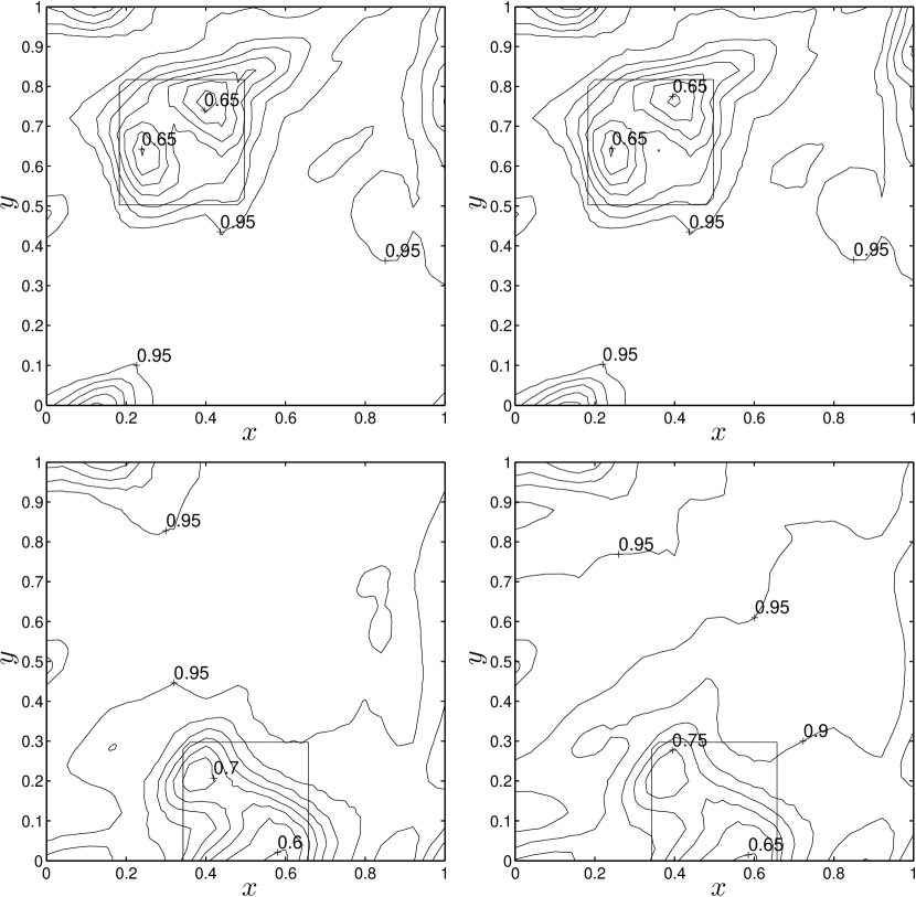
Figure 7. 2D reconstruction using the weighted average (32), final time $T=1.5$ and Neumann boundary condition $2\sin(4\pi t)$ for $x\in[0.4,0.6]$, $t<0.5$ and $0$ elsewhere. The data $u^{*}$ was simulated by solving the forward equation on a quasi-uniform mesh with 3232 triangles and 328 time steps while the inverse problem was solved on a uniform mesh with 1250 triangles and 30 time steps. Measurements from the whole boundary were used. Top: Reconstruction of $\sigma_{true}=0.5$ inside the square $[0.2,0.5]\times[0.5,0.8]$ and $\sigma_{true}=1$ elsewhere, with no noise in data (left) and 10% noise in data (right). Bottom: Reconstruction of $\sigma_{true}=0.5$ inside the square $[0.35,0.65]\times[0,0.3]$ and $\sigma_{true}=1$ elsewhere, with no noise in data (left) and 10% noise in data (right).

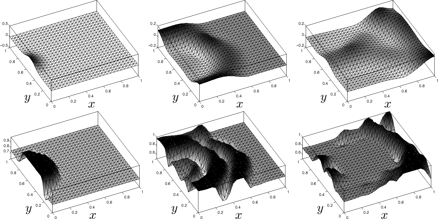
Figure 8. Measurements $u^{*}$ (top) and $\mathfrak{h}_{\delta}^{\prime}(\nabla u\cdot\nabla q)$ (bottom) for timesteps 5, 15 and 25. The data here corresponds to the top left plot in Figure 7, and $u^{*}$ is interpolated onto the mesh used for the calculation of $u$ and $q$.

References

• [1] H. T. Banks and K. Kunisch. Estimation techniques for distributed parameter systems, volume 1 of Systems & Control: Foundations & Applications. Birkhäuser Boston Inc., Boston, MA, 1989.
• [2] Emmanuel Nicholas Barron and Robert Jensen. The Pontryagin maximum principle from dynamic programming and viscosity solutions to first-order partial differential equations. Trans. Amer. Math. Soc., 298(2):635–641, 1986.
• [3] M. P. Bendsøe and O. Sigmund. Topology optimization. Springer-Verlag, Berlin, 2003. Theory, methods and applications.
• [4] Michele Benzi, Gene H. Golub, and Jörg Liesen. Numerical solution of saddle point problems. Acta Numer., 14:1–137, 2005.
• [5] George Biros and Omar Ghattas. Parallel Lagrange-Newton-Krylov-Schur methods for PDE-constrained optimization. I. The Krylov-Schur solver. SIAM J. Sci. Comput., 27(2):687–713 (electronic), 2005.
• [6] Liliana Borcea. Electrical impedance tomography. Inverse Problems, 18(6):R99–R136, 2002.
• [7] Jesper Carlsson. Pontryagin approximations for optimal design of elastic structures. preprint, 2006.
• [8] Jesper Carlsson, Mattias Sandberg, and Anders Szepessy. Symplectic pontryagin approximations for optimal design. Preprint.
• [9] M. G. Crandall, L. C. Evans, and P.-L. Lions. Some properties of viscosity solutions of Hamilton-Jacobi equations. Trans. Amer. Math. Soc., 282(2):487–502, 1984.
• [10] Heinz W. Engl, Martin Hanke, and Andreas Neubauer. Regularization of inverse problems, volume 375 of Mathematics and its Applications. Kluwer Academic Publishers Group, Dordrecht, 1996.
• [11] FEniCS. FEniCS project. URL: urlhttp//www.fenics.org/.
• [12] Ernst Hairer, Christian Lubich, and Gerhard Wanner. Geometric numerical integration, volume 31 of Springer Series in Computational Mathematics. Springer-Verlag, Berlin, second edition, 2006. Structure-preserving algorithms for ordinary differential equations.
• [13] J. Hoffman, J. Jansson, A. Logg, and G. N. Wells. DOLFIN. URL: urlhttp//www.fenics.org/dolfin/.
• [14] J.-L. Lions. Optimal control of systems governed by partial differential equations. Translated from the French by S. K. Mitter. Die Grundlehren der mathematischen Wissenschaften, Band 170. Springer-Verlag, New York, 1971.
• [15] M. Sandberg and A. Szepessy. Convergence rates of symplectic Pontryagin approximations in optimal control theory. M2AN, 40(1), 2006.
• [16] Mattias Sandberg. Convergence rates for numerical approximations of an optimally controlled Ginzburg-Landau equation. preprint, 2006.
• [17] Curtis R. Vogel. Computational methods for inverse problems, volume 23 of Frontiers in Applied Mathematics. Society for Industrial and Applied Mathematics (SIAM), Philadelphia, PA, 2002. With a foreword by H. T. Banks.