Ultra-High-Energy Cosmic Rays from the Radio Lobes of AGNs

Abstract

In the past year, the HiRes and Auger collaborations have reported the discovery of a high-energy cutoff in the ultra-high energy cosmic-ray (UHECR) spectrum, and an apparent clustering of the highest energy events towards nearby active galactic nuclei (AGNs). Consensus is building that such $\sim 10^{19}$–$10^{20}$ eV particles are accelerated within the radio-bright lobes of these sources, but it is not yet clear how this actually happens. In this paper, we report (to our knowledge) the first treatment of stochastic particle acceleration in such environments from first principles, showing that energies $\sim 10^{20}$ eV are reached in $\sim 10^{6}$ years for protons. However, our findings reopen the question regarding whether the high-energy cutoff is due solely to propagation effects, or whether it does in fact represent the maximum energy permitted by the acceleration process itself.

1 Introduction

Cosmic rays are energetic charged particles traveling throughout the Galaxy and the intergalactic medium under the influence of various physical processes, including deflection by magnetic fields, and collisions with other particles along their trajectory. Their energy spectrum measured at Earth is a steep (roughly power-law) distribution with logarithmic index $\alpha\sim 2.6$–3, extending up to a few times $10^{20}$ eV. Other than their spectrum, these particles are characterized by their angular distribution in the sky, and by their mass composition.

A highly significant steepening in the UHECR spectrum was reported by both the HiRes (Abbasi et al. 2008) and Auger (2008c) collaborations. (Distinguished from their lower-energy counterparts, UHECRs have energies in excess of 1 EeV $\equiv 10^{18}$ eV.) This result may be a strong confirmation of the predicted Greisen-Zatsepin-Kuzmin (GZK) cutoff due to photohadronic interactions between the UHECRs and low-energy photons in the cosmic microwave background (CMB) radiation (Greisen 1966; Zatsepin & Kuz’min 1966). Together with the measured low fraction of high-energy photons in the CR distribution, this measurement already rules out so-called top-down models, in which the UHECRs represent the decay products of high-mass dark matter particles created in the early Universe (Semikoz et al. 2007). The measured photon flux is also in conflict with scenarios in which UHECRs are produced by collisions between cosmic strings or topological defects (Bluemer et al. 2008, Auger 2008b). On the other hand, such energetic particles may still be produced via astrophysical acceleration mechanisms (see Torres & Anchordoqui 2004 and other references cited therein).

UHECRs are not detected directly, but through the showers they create in Earth’s atmosphere (see, e.g., Melia 2009). Depending on the energy and type of primary particle, the ensuing cascade has characteristics that allow the ground-based observatories to determine not only whether the incoming UHECR is a photon, but also its atomic number. It should be pointed out, however, that a determination of the primaries’ composition strongly relies on an extrapolation of current phenomenological hadronic interaction models, so it remains rather uncertain. The Auger (2007) data confirmed the dominance of protons in primary cosmic rays, though they also exhibit evidence for a mixed composition extending to energies as high as $\sim$ 50–60 EeV, with a higher atomic number $Z$, up to $Z\sim 26$ (Unger et al. 2007).

But the most telling indicator for the possible origin of these UHECRs is the discovery by Auger (Auger 2008a) of their clustering towards nearby ($\sim 75$ Mpc) AGNs along the supergalactic plane. The significance of this correlation has been further strenghtened by a more recent analysis which weights the AGN spatial distribution by their hard X-ray flux (George et al. 2008). This raises at least two questions: (1) How are the UHECRs accelerated to such high energies? and (2) given these nearby sources, is the sharp suppression of UHECRs in the last decade of their observed energies really due solely to the GZK effect, or does it signal a limitation to the acceleration efficiency?

Previous attempts at understanding how particles are accelerated to EeV energies and beyond have generally been based on first-order Fermi acceleration (see, e.g., Ostrowski 2008, and other references therein) within shocks created by blast waves like those in supernova remnants (Fatuzzo & Melia 2003, Crocker et al. 2005). But this process is subject to kinematic restrictions that inhibit the particles from actually reaching ultra-high energies (see, e.g., Nayakshin & Melia 1998, Gallant et al. 1999). Recent numerical simulations have shown that an increase in the Lorentz factor $\gamma$ of ultra-relativistic shock waves steepens the observed spectrum (Niemiec & Ostrowski 2006) and reduces its high-energy cutoff.

For these reasons, it is not plausible for UHECRs to emerge from astrophysical environments, such as supernova remnants, where first-order processes are dominant so long as the shock velocity is super-Alfvénic, because they cannot even contain such high-energy particles (Hillas 1984)—the gyration radius of particles with energy $\sim 10^{20}$ eV for a typical galactic magnetic field is much larger than the size ($<10$ pc) of these structures.

On the other hand, a second-order Fermi process (Fermi 1949) can explain observational features not addressed by the first-order process, as in the case of a supernova remnant itself (see Cowsik & Sarkar 1984). Moreover, stochastic particle acceleration through a gyroresonant interaction with MHD turbulence (a second-order Fermi process; see Fermi 1949) can be very efficient if the Alfvén velocity approaches $c$ (Dermer & Humi 2001). The stochastic acceleration of particles by turbulent plasma waves has already received some attention in the literature (see Liu et al. 2004, 2006, and references cited therein, and Wolfe & Melia 2006). Indeed, the feasibility of second-order Fermi acceleration in radio galaxies has been demonstrated through the steady re-acceleration of electrons in certain hot spots (Almudena Prieto et al. 2002).

Our treatment from first principles, however, avoids many of the previously encountered unknowns and limitations. In this paper, we report (to our knowledge) the first treatment of stochastic acceleration of charged particles in the lobes of radio-bright AGNs by directly computing the trajectory of individual particles. An earlier version of this treatment—for the propagation of charged particles assumed already accelerated at TeV energy through the turbulent magnetic field at the Galactic centre—may be found in Ballantyne et al. 2007, and Wommer, Melia & Fatuzzo 2008; by contrast, in the present paper both the propagation and acceleration are taken into account. We show that random scatterings (a second-order Fermi process) between the charges and fluctuations in a turbulent magnetic field can accelerate these particles up to ultra-high energies, provided a broad range of fluctuations is present in the system.

2 Description of the model

In our treatment, we follow the three-dimensional motion of individual particles within a time-varying turbulent magnetic field. By avoiding the use of equations describing statistical averages of the particle distribution, we mitigate our dependence on unknown factors, such as the diffusion coefficient. We also avoid such limitations as the Parker approximation (Padmanhaban 2001) in the transport equation. However, a remaining unknown is the partitioning between turbulent and background fields. For simplicity, we take the minimalist approach and assume that the magnetic energy is divided equally between the two components.

Another unknown is the turbulent distribution. For many real astrophysical plasmas, the magnetic turbulence seems to be in accordance with the Kolmogorov spectrum. This is seen, e.g., in the solar wind (Leamon et al. 1998) and through interstellar scintillation (Lee & Jokipii 1976); a more recent numerical analysis of MHD turbulence confirms the general validity of the Kolmogorov power spectrum (Cho et al. 2003). In addition, renormalization group techniques applied to the analysis of MHD turbulence also favour a Kolmogorov power spectrum (for more details, see Smith et al. 1998, and Verma 2004).

We model the radio lobe of an AGN as a sphere of radius ${\mathcal{R}}$, a second parameter in our simulations. A population of relativistic particles of mass $m$, protons or heavy ions, with an energy $E=\gamma mc^{2}$, where $\gamma$ is the Lorentz factor, is released in an inner sphere of radius ${\mathcal{R}^{\prime}}\sim\alpha{\mathcal{R}}$. The value of $\alpha$ must be much smaller than 1, otherwise very few particles reach an energy $E>10^{18}$eV. For a small value of $\alpha$, the gyration radius becomes comparable to the size of the acceleration region at $E>10^{18}$eV, and therefore changes in $\alpha$ do not significantly alter the result. For the sake of specificity, we use a value $\alpha\sim 10^{-3}$ in this paper. Once released, the particles propagate through the turbulent field until they escape the acceleration region and enter intergalactic space.

2.1 Time varying turbulent field

We use the Giacalone & Jokipii (1994) prescription for generating the turbulent magnetic field. Their principal aim of propagating individual particles through a magnetostatic field was to compute the Fokker-Planck coefficients for a direct comparison with analytic theory. For our purpose, we modify that prescription to include a time-dependent phase factor that allows for temporal variations.

The global magnetic field is written as a sum of a background term $\mathbf{B}_{0}$, constant and uniform, and a turbulent field varying in space and time (i.e., as a superposition of Alfvén waves).

The equation of motion of a relativistic test particle with charge $e$ and mass $m$ moving in an electromagnetic field $F^{\mu\nu}$ is the Lorentz equation (Landau & Lifchitz 1975, Melia 2001)

$$mc\frac{du^{\mu}}{ds}=\frac{e}{c}F^{\mu\nu}u_{\nu}$$ (1)

(with $\mu=0,1,2,3$), where $c$ is the speed of light in vacuum, $u^{\mu}=\left(\gamma,\gamma{\mathbf{v}}/{c}\right)$ is the four-velocity of the particle, $\gamma=1/\sqrt{1-(v/c)^{2}}$ is the Lorentz factor, and $s/c$ is the proper time. We calculate the trajectory of the particle in a magnetic field $\mathbf{B}(t,\mathbf{r})=(mc/e)\mathbf{\Omega}(t,\mathbf{r})$ as a solution of the space components ($\mu=1,2,3$) of Equation (1)

$$\frac{d\mathbf{u}(t)}{dt}=\delta\mathbf{\cal E}(t,\mathbf{r})+\frac{\mathbf{u}(t)\times\mathbf{\Omega}(t,\mathbf{r})}{\gamma(t)}\;,$$ (2)

where $t$ is the time in the rest frame of the acceleration region. The quantity $\mathbf{\Omega}(t,\mathbf{r})$ in Equation (2) is given by

$$\mathbf{\Omega}(t,\mathbf{r})=\mathbf{\Omega}_{0}+\delta\mathbf{\Omega}(t,\mathbf{r})\;,$$ (3)

where $\mathbf{\Omega}_{0}\equiv(e/mc)\mathbf{B}_{0}$, in terms of the background magnetic field $\mathbf{B}_{0}$, and $\delta\mathbf{\Omega}(t,\mathbf{r})$ is the time-dependent turbulent magnetic field. We ignore any large-scale background electric fields—a reasonable assumption given that currents would quench any such fields within the radio lobes of AGNs. The time variation of the magnetic field, however, induces an electric field $\delta\mathbf{\cal{E}}(t,\mathbf{r})\equiv(e/mc)\mathbf{E}(t,\mathbf{r})$ according to Faraday’s law.

The procedure of building the turbulence calls for the random generation of a given number $N$ of transverse waves $\mathbf{k}_{i}$, $i=1,..,N$ at every point of physical space where the particle is found, each with a random amplitude, phase and orientation defined by angles $\theta(k_{i})$ and $\phi(k_{i})$. This form of the fluctuation satisfies $\nabla\cdot\delta\mathbf{\Omega}(t,\mathbf{r})=0$. We write

$$\delta\mathbf{\Omega}(t,\mathbf{r})=\sum_{i=1}^{N}\Omega(k_{i})\hat{\xi}_{\pm}(k_{i})e^{\left[i(k_{i}x^{\prime}-\omega_{i}t+\beta(k_{i}))\right]}\;,$$ (4)

where the polarization vector is given by

$$\hat{\xi}_{\pm}(k_{i})=\cos\alpha(k_{i})\hat{\bf y}^{\prime}\pm i\sin\alpha(k_{i})\hat{\bf z}^{\prime}\;.$$ (5)

Given the form in Equation (4) for the turbulence, the electric field $\delta\mathbf{\cal{E}}(t,\mathbf{r})$ is given by

$$\delta\mathbf{\cal{E}}(t,\mathbf{r})=\sum_{i=1}^{N}\Omega(k_{i})\frac{\omega(k_{i})}{k_{i}c}\hat{\xi}_{\pm}^{E}(k_{i})e^{\left[i(k_{i}x^{\prime}-\omega_{i}t+\beta(k_{i}))\right]}\;,$$ (6)

with

$$\hat{\xi}_{\pm}^{E}(k_{i})=\pm i\sin\alpha(k_{i})\hat{\bf y}^{\prime}-\cos\alpha(k_{i})\hat{\bf z}^{\prime}\;.$$ (7)

The orthonormal primed coordinates ${\bf r^{\prime}}=(\hat{x}^{\prime},\hat{y}^{\prime},\hat{z}^{\prime})$ are related to the lab-frame coordinates ${\bf r}=(\hat{x},\hat{y},\hat{z})$ via the rotation matrix $R(\theta,\phi)$, in such a way that for every $k$ the propagation vector is parallel to the $\hat{x}^{\prime}$ axis. The matrix $R(\theta,\phi)$ is given by

$${\bf r^{\prime}}=\left(\begin{array}[]{ccc}\cos\theta\;\cos\phi&\cos\theta\;\sin\phi&\sin\theta\\ -\sin\phi&\cos\phi&0\\ -\sin\theta\;\cos\phi&-\sin\theta\;\sin\phi&\cos\theta\\ \end{array}\right){\bf r}\;.$$ (8)

For each value of $k_{i}$, there are 5 random numbers: $0<\theta(k_{i})<\pi$, $0<\phi(k_{i})<2\pi$, $0<\alpha(k_{i})<2\pi$, $0<\beta(k_{i})<2\pi$ and the sign plus or minus indicating the sense of polarization.

Further assumptions are necessary to specify the dispersion relation $\omega=\omega(k_{i})$. For every turbulent mode, we use the dispersion relation for transverse non-relativistic Alfvén waves (see Kaplan & Tsytovich 1973 for an extended discussion): $\omega(k_{i})=v_{A}k_{i}\cos\theta(k_{i})$, for $i=1,..,N$, where $v_{A}=B_{0}/\sqrt{4\pi m_{p}n}$ is the non-relativistic Alfvén velocity in a medium with background magnetic field $B_{0}$ and number density $n$, $m_{p}$ the proton mass, and $\theta(k_{i})$ is the angle between the wavevector $\mathbf{k}_{i}$ and $\mathbf{B}_{0}$. This is the condition thought to be valid for the propagation of turbulent modes in a magnetized astrophysical environment, such as the radio lobes of an AGN. The background plasma is assumed to have a background proton number density $n\sim 10^{-4}$ cm^-3, a reasonable value for these environments (Almudena Prieto et al. 2002).

The amplitudes of the magnetic fluctuations are assumed to be consistent with Kolmogorov turbulence, so

$$\Omega(k_{i})=\Omega(k_{min})\left(\frac{k_{i}}{k_{min}}\right)^{-\Gamma/2}\;,$$ (9)

for $i=1,..,N$, where $k_{min}$ corresponds to the longest wavelength of the fluctuations and the index $\Gamma$ of the power spectrum $\Omega^{2}(k)$ is $5/3$. Finally, the quantity $\Omega(k_{min})$ is computed by requiring that the energy density of the magnetic fluctuations equals that of the background magnetic field:

$$S=\sum_{i=1}^{N}\frac{B^{2}(k_{i})}{8\pi}=\frac{m^{2}c^{2}}{8\pi e^{2}}\Omega^{2}(k_{min})\sum_{i=1}^{N}\left(\frac{k_{i}}{k_{min}}\right)^{-\Gamma}=\frac{{B_{0}}^{2}}{8\pi}.$$

(10)

We choose N=2400 values of $k$ evenly spaced on a logarithmic scale; i.e., a wavenumber shell with bounds $k_{i}-k_{i+1}$ holds $k_{i+1}=k_{i}\times(k_{max}/k_{min})^{1/N}$ values. Considering that the turbulence wavenumber $k$ is related to the turbulent length scale $l$ by $k=2\pi/l$, we adopt a range of lengthscales from $l_{min}=10^{-1}\,v_{0}/\Omega_{0}$ to $l_{max}=10^{9}\,v_{0}/\Omega_{0}$, where $v_{0}$ is the initial velocity of the particle and $\Omega_{0}$ is the initial gyrofrequency in the background magnetic field. Thus the dynamic range covered by $k$ is $k_{max}/k_{min}=l_{max}/l_{min}=10^{10}$, and our description allows for $240$ transverse modes $k$ per decade. The values of $k_{max}$ and $k_{min}$ fix the magnetic energy equipartition through Equation (10). The value ${k_{min}}^{-1}$ is proportional through a factor of order $1$ to the correlation length of the turbulence (see Ruffert and Melia 1994, and Rockefeller et al. 2004, for examples of how this is generated in the interstellar medium); the value ${k_{max}}^{-1}$ is the wavelength at which the interaction between the turbulence and most of the particles is the most efficient, so that energy is drained out of $\delta\Omega$.

However, since the gyroradius $r_{g}(E)$ evolves over a large energy interval, the gyroresonant wavenumber $k_{res}(E)$ moves accordingly in such a way that in the global wavenumber interval $(k_{min}-k_{max})$ there is for every $E$ a certain $k_{res}(E)$ fulfilling the resonance condition $r_{g}(E)k_{res}(E)\sim 1$. Such a $k$ range involves a large computational time, especially if a statistically significant number of particles is to be considered.

Since our numerical simulation is not performed by specifying the magnetic turbulence on a computational grid with given cell size $\Delta x$, the choice of $k_{max}=2\pi/l_{min}$ is not dictated by a fixed spatial resolution (see section 3 for more details). In addition, the result is not affected by spurious effects to the discreteness or the periodicity. As a byproduct, the divergenceless condition $\nabla\cdot\delta\mathbf{\Omega}(t,\mathbf{r})=0$ is easily satisfied and does not require an extension of the Godunov solver of the MHD equations for the purpose of “divergence cleaning” (Ryu et al. 1998) or a reformulation of the MHD equations including, e.g., divergence-damping terms (Dedner et al. 2002).

With this prescription, we construct the turbulent magnetic field at every point of physical space where the particle is found, which we then propagate without taking any time-average along the trajectory. The particles passing through this region are released initially at a random position inside the acceleration zone, which for simplicity is taken to be a sphere of radius ${\mathcal{R}}$, with a fixed initial velocity $v_{0}$ pointed in a random direction. The initial value of the Lorentz factor $\gamma_{0}=1/\sqrt{1-(v_{0}/c)^{2}}\simeq 1.015$ is chosen to avoid having to deal with ionization losses for the protons or heavy ions. The particles closest to the edge of the acceleration zone have a higher probability of escaping than those starting farther in, and therefore reach relatively lower energies. In the usual (Fermi) way, this produces (in the highest energy portion of the spectrum) an inverted power-law distribution.

2.2 Energy losses

In principle, energy losses due to synchrotron and inverse Compton processes involving radio and Cosmic Microwave Background (CMB) photons, all of which increase as $\gamma^{2}$, can significantly limit the maximum energy attainable by a cosmic ray during the acceleration process, given that its Lorentz factor $\gamma$ evolves from $\sim 1$ up to $10^{10}-10^{11}$. For an UHE particle (either a proton or a heavy ion), both the radio and CMB photons will have an energy $\gamma h\nu$ in the centre-of-momentum frame well below the rest energy of the cosmic ray (i.e., $\gamma h\nu<<mc^{2}$, where $m$ is the mass of the accelerating particle). For the purpose of these estimates, we use a radio frequency $\nu_{radio}=0.1$ GHz ($h\nu_{radio}\sim 4.2\times 10^{-7}$ eV) and a CMB frequency corresponding to the peak of the blackbody spectrum, $\nu_{CMB}=2.821kT/h=158$ GHz ($h\nu_{CMB}\sim 6.6\times 10^{-4}$ eV), where $k$ is the Boltzmann constant, $h$ the Planck constant, and $T=2.7$ K is the CMB temperature. Consequently, the energy losses due to inverse Compton may be calculated in the Thomson limit. Compare this with the situation for high energy electrons, for which the Thomson condition would not be satisfied even at energies $\gamma m_{e}c^{2}\sim 10^{16}$ eV, requiring in that case the full Klein-Nishina treatment.

The propagation of high-energy particles is here modeled in a region of tens of kpc size. Therefore we neglect any effect of the relativistically-narrowed jet on the spatial distribution of the radio background, assumed for simplicity to be isotropic. Since the CMB intensity field is also isotropic, we take these energy losses into account using the following angle-integrated power-loss rate:

$$-\frac{dE}{dt}=\frac{4}{3}\sigma_{T}(m)c\gamma^{2}\left(\frac{B^{2}}{8\pi}+U_{R}+U_{CMB}\right)\;,$$ (11)

where $\sigma_{T}(m)=6.6524\times(m_{e}/m)^{2}\,10^{-25}$ cm² is the Thomson cross section for a generic particle of mass $m$, which can be a proton or heavy ion, and $B^{2}/(8\pi)=(2{B_{0}}^{2})/(8\pi)$ is the total energy density of the magnetic field. The photon energy density $U_{R}$ inside a typical radio lobe is computed as $U_{R}=L/(4\pi c{\mathcal{R}}^{2})$, where we assume $L$ to be a standard luminosity density corresponding to the Fanaroff-Riley class II of galaxies ($L=5\times 10^{25}$ W Hz^-1 sr^-1 at $178$ MHz), and ${\mathcal{R}}$ is the size of the spherical acceleration zone. For the CMB, we use $U_{CMB}=aT^{4}=4.2\times 10^{-13}$ erg cm^-3. In a region where magnetic turbulence is absent or static, a given test particle propagates by “bouncing” randomly off the inhomogeneities in $\mathbf{B}$, but its energy remains constant. The field we will model below, however, is comprised of time-varying gyroresonant turbulent waves (see Equation 4), and collisions between the test particle and these waves produces a net acceleration (in the lab frame).

Figure 1: Three-dimensional trajectory of single particle in the turbulent field of Giacalone & Jokipii (1994) reproduced with our code. The length scales are in units of the gyration radius, $v_{0}/{\Omega_{0}}$, which remains constant during the propagation. The energy is verified to be constant, as expected, over a time interval $\Delta t=1000{\Omega_{0}}^{-1}$, within a relative error of $10^{-5}$. The background magnetic field $B_{0}$ is parallel to the $z$ axis and, as found by Giacalone & Jokipii (1994), the diffusion along ${\bf B}_{0}$ dominates with respect to that across the field.

Figure 2: Three-dimensional trajectory of a single particle released at random within the acceleration zone, assumed to be a sphere of radius 50 kpc. The scale on the axes is in units of $10^{8}v_{0}/\Omega_{0}$, where $v_{0}/\Omega_{0}$ is the initial gyroradius. The particle is released with a fixed initial speed $v_{0}$, but pointed in a randomly chosen direction. The calculation stops when the particle leaves the radio lobe and is injected into the intergalactic medium.

3 Numerical code setup

In this section we describe the numerical code used to perform the simulations. The Lorentz Equation (2) is integrated using a Runge-Kutta $4^{th}$ order method (Press et al. 1997) for the system of 6 first-order differential equations

$$\frac{{\rm d}{\bf x_{i}}}{{\rm d}t} = \frac{c}{\gamma}{\bf u_{i}}$$ (12)

$$\frac{d\mathbf{u_{i}}}{dt} = \delta\mathbf{\cal{E}}_{i}+\frac{[\mathbf{u}\times\mathbf{\Omega}]_{i}}{\gamma}\;,$$ (13)

for $i=1,2,3$. The components $\delta\mathbf{\cal{E}}_{i}$ and $\mathbf{\Omega}_{i}$ are intended to be the real parts of the corresponding complex quantities.

The portable random number generator used to produce the turbulence is Knuth’s subtractive routine ran3 (Press et al. 1997), with a seed number $I=10^{9}$. This routine has a relatively short execution time and is suitable to avoid the introduction of unwanted correlations into the numerical computation.

There are two approaches to numerically implementing a turbulent magnetic field generated by this method. The first approach (used in Giacalone & Jokipii 1994) is to calculate the magnetic field at every time step for each particle position. The position is then found by solving the Lorentz Equation (2). In the second approach, the magnetic field is generated for a given volume at the beginning of the simulation and then it evolves according to Equation (4). In order to have an acceptable $k$-binning with a dynamical range of $k_{max}/k_{min}=10^{10}$, one would then need to specify the field at an excessively large number of lattice points. This is not only time-consuming, but also very memory-intensive. So, like Giacalone & Jokipii (1994), we adopt the former approach. In this way, the magnetic field is generated only where needed, and the overwhelming amount of computer memory required by the second approach is not necessary,. Since the confinement volume is a parameter of the model, the second approach would also require adapting the lattice spacing in order to maintain the same space resolution in physical space.

The Runge-Kutta integrator has previously been validated for the cases of uniform and constant electric and magnetic fields, where the outcome of the simulation can be compared with an analytical solution.

Secondly, as a validation test of the code, we reproduced the result of Giacalone & Jokipii (1994) for the case of a 3D magnetostatic turbulence, by using the same set of parameters. We discretize the turbulence in 50 transverse modes $k$, where the values of $k$ are chosen to be evenly spaced in logarithmic scale in the interval of the corresponding length scales from $l_{min}=(1/5)\,v_{0}/\Omega_{0}$ to $l_{max}=10\,v_{0}/\Omega_{0}$, where $v_{0}$ is the initial velocity of the particle and $\Omega_{0}$ is its gyrofrequency in the background magnetic field. The particles are released in a random initial position with initial velocity randomly oriented but with fixed value $v_{0}$. In Figure 1, we present the trajectory of a single particle, the position along the three axes expressed in units of the gyration radius. In this test, the energy of the particle is constant within a relative error of $10^{-5}$ over a time interval corresponding to $10^{3}\Omega_{0}^{-1}$.

In order to produce the time-dependent turbulent magnetic field considered in this paper, between two successive shufflings of all five random quantities in $\delta\mathbf{\Omega}$, which are performed every $\Delta t\sim 10^{8}-10^{9}$s, the particle propagates gyroresonantly with the oscillating turbulence. We verified that a change in the Runge-Kutta time-binning by over one order of magnitude does not produce any systematic numerical effects associated with $\gamma(t)$ and the spectrum. Changing the $k$-binning from $N=1200$ to $N=3000$ in Equation 4 similarly does not noticeably change the resultant $\gamma(t)$ and the spectrum. We chose $N=2400$ which results in a reasonably long computational time. However, a coarser $k$-binning, e.g., with $10$ modes/decade, could possibly result in a worse determination of the macroscopic indicator as instantaneous spatial diffusion coefficients; the time evolution of the diffusion coefficients is however beyond the scope of the present paper.

Figure 3: Simulated time evolution of the Lorentz factor $\gamma$ for a proton propagating through a time-varying turbulent magnetic field. The three curves correspond to three different values of $B_{0}$: $10^{-7}$, $10^{-8}$, and $10^{-9}$ gauss. The protons are released at an initial random position inside the acceleration zone—a sphere of radius ${\mathcal{R}}=50$ kpc—with the same initial speed $v_{0}$, though pointed in random directions. The proton is followed until it leaves the acceleration zone and enters the intergalactic medium. The acceleration timescale $\Delta t$ is inversely proportional to the background field $B_{0}$. Therefore, as expected, a larger $B_{0}$ produces a more efficient acceleration. In this example, a proton winding its way through a field $B_{0}=10^{-8}$ gauss attains an energy $E\sim 10^{20}$ eV in approximately $10^{6}$ years.

4 Results and discussion

Figure 2 (to be compared with Figure 1) shows the trajectory of a single particle released at random within the acceleration zone, with the initial speed $v_{0}$, pointed in random direction, with an ambient magnetic field $B_{0}=10^{-8}$ gauss. In Figure 3, we plot the time evolution of the particle Lorentz factor $\gamma$ for three representative values of the background field $B_{0}$: $10^{-7}$, $10^{-8}$, and $10^{-9}$ gauss. We see the particle undergoing various phases of acceleration and deceleration as it encounters fluctuations in $\mathbf{B}$.

The acceleration of the particle results from the 0-$th$ component of Equation 1, which reads

$$\frac{d\gamma}{dt}=\frac{\delta\mathbf{\cal E}^{i}u_{i}}{\gamma},$$ (14)

where $\delta\mathbf{\cal E}^{i}u_{i}$ is the scalar product of the electric field and the 3-velocity of the particle. Therefore the acceleration is given by $\gamma(t)=\sqrt{{\gamma_{0}}^{2}+2\int_{t_{0}}^{t}\delta\mathbf{\cal E}^{i}u_{i}dt^{\prime}}$. The integrand function can be strongly time-varying and therefore needs to be computed numerically.

As can be seen in Figure 3, the acceleration timescale $\Delta t_{acc}$ is inversely proportional to $B_{0}$ so, as expected, more energetic turbulence accelerates the particles more efficiently, in agreement with what was expected from the non-relativistic Alfvén wave theory. Previous studies (Casse et al. 2002) of particle transport through a turbulent magnetic field using the prescription in Giacalone & Jokipii (1994), compared with a Fast Fourier Transform method, showed that the time of confinement within the jets of FR II galaxies is too small for the particles to attain an energy of $10^{20}$ eV. In our case, the particle acceleration takes place over a much bigger volume (with dimension ${\mathcal{R}}=50$ kpc, compatible with the known size of FR-II radio galaxies) and the efficiency is enhanced by the strong temporal variation of the turbulence. We find, in particular, that particles can easily accelerate to UHE on timescales short compared to the age of the radio-lobe structure through a gyroresonant interaction with a magnetic turbulence.

In our simulation, the particle acceleration is efficient because it occurs over a wide range of turbulent fluctuations, such that the wave-particle interaction is resonant at all times. Such a distribution is expected if the magnetic energy cascade proceeds (without loss) from the largest spatial scales down to the region where energy dissipation and transfer to the particles becomes most efficient.

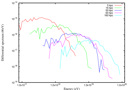
Figure 4: Calculated differential spectra for 500 protons with $B_{0}=10^{-8}$ gauss and for different values of the size of the acceleration region, assumed to be a sphere of radius spanning the interval ${\mathcal{R}}=[5-160]$ kpc. The dependence of the energy cutoff on ${\mathcal{R}}$ is evidenced. This result shows that the cutoff in the observed spectral distribution can be due to the competition between two distint effects: propagation through the CMB and intrinsic properties of the accelerator. Moreover, the slope in the region $E>4\times 10^{18}$ eV strongly depends on $R$. This diagram supports the view that the steeper CR spectrum below $\log(E/eV)\approx 18.6$ likely represents a population of galactic cosmic rays.

In Figures 4 and 5 we show the spectral distributions for distinct values of the turbulent energy and size of the acceleration region. In order to produce this result, we followed the trajectory of 500 protons, launched in the manner described above, with different values of the parameters $R$ and $B_{0}$.

We conclude that the observed spectral cutoff (Abbasi et al. 2008, Auger 2008b) can result from the competition of two distint effects: not only the GZK cutoff, namely degradation of primary UHECRs due to the propagation through the CMB, but also, and possibly dominant, intrinsic properties of the source which constrain the process of acceleration.

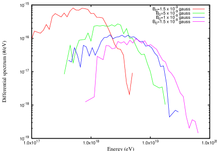
Figure 5: Calculated differential spectra for 500 protons with $R=50$ kpc and for different values of the turbulent magnetic energy. In this case $B_{0}$ spans the interval $B_{0}=1.5\times[10^{-9}-10^{-8}]$ gauss. See the comments in Figure 4.

Figure 6 depicts the calculated differential spectrum in the energy range $\log(E/{\rm eV})=[18.6-19.5]$. From our sampling of the various physical parameters, we infer that for a radius ${\mathcal{R}}=50$ kpc, $B_{0}$ should lie in the range $[0.5-5]\times 10^{-8}$ gauss in order to produce UHECRs with the observed distribution shown in this figure.

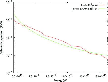
Figure 6: Calculated differential spectrum for 1,000 protons in the energy range $\log(E/eV)=[18.6-19.5]$ for the selected parameters $B_{0}=10^{-8}$ gauss and ${\mathcal{R}}=50$ kpc. A power-law behaviour with index $-2.6$ in the differential spectrum of protons injected into the intergalactic medium in this model is in agreement with a recent statistical analysis of HiRes observations (Gelmini et al. 2007). This good match supports the view that the steeper CR spectrum below $\log(E/eV)\approx 18.6$ represents a different population, possibly associated with the Galaxy itself.

It is worth emphasizing that this calculation was carried out without the use of several unknown factors often required in approaches solving the hybrid Boltzmann equation to obtain the phase-space distribution function for the particles. In addition, we remark that the acceleration mechanism we have invoked here is sustained over 10 orders of magnitude in particle energy, beginning at $\gamma\sim 1$; the UHECRs therefore emerge naturally from the physical conditions thought to be prevalent within the giant radio lobes of AGNs, without the introduction of any additional exotic physics (for a complete review of the bottom-up models, see Bhattacharjee & Sigl 2000 and other references cited therein).

To provide the possibility of observationally testing the model we have presented here, we show in Figure 7 the temporal evolution of the energy loss rate to first order in $\gamma h\nu/(m_{e}c^{2})$ (Blumenthal & Gould 1970) for a single electron propagating through the same magnetic turbulence we have used to accelerate the protons and heavier ions. By estimating the flux of UHE protons $\dot{N}_{p}$ escaping from one giant radio lobe, under the assumption of neutrality in the source, we can estimate the flux of accelerated electrons $\dot{N}_{e}$. In principle, it is therefore possible to estimate the expected radio luminosity from these regions due to this particular acceleration process.

Figure 7: Energy loss rate of a single electron in a turbulent time-varying magnetic field with $B_{0}=10^{-8}$ gauss. In this diagram both the energy losses due to synchrotron and inverse Compton on the Radio and CMB photons in the acceleration region are shown. Unlike the case of protons and heavy ions, the radiation rate for an electron exceeds the acceleration rate in such a way that, for the given $B_{0}$, in a time of order of $10$ years the electron will have lost all of its energy.

We should point, however, that though a comparison of our results with the observations supports the viability of this model, our calculations are subject to several factors we have not fully explored here. For example, the observed spectrum may be affected by the cosmological evolution in source density (Berezinsky et al. (2006)). However, this omission will not be overly constraining since a likelihood analysis (Gelmini et al. (2007)) of the dependence of the observed distribution on input parameters has already shown that, in the case of protons, for $m\sim 0$, where $m$ is the evolution index in the source density, the HiRes observations are compatible with a power-law injection spectrum with index $-2.6$. The analysis of the Auger data seems to confirm this (Auger (2008c)). Thus, although source-density evolution may alter our results somewhat, our conclusions will probably not be greatly affected. In a more conservative interpretation, the result presented here provides the injection spectrum from a single source.

Second, we have not included the GZK effect for particle energies above 50 EeV. This omission becomes progressively more important as the energy approaches $10^{20}$ eV. These refinements, in addition to a more detailed analysis of the composition of primary UHECRs, will be reported in a forthcoming paper. Any discussion concerning the evolution of the instantaneous spatial diffusion coefficients parallel to and perpendicular to the background magnetic field, and on the transition to a diffusive regime, will also be reserved to a future publication.

In our approach, we have also neglected the backreaction of the accelerated particles on the turbulent field which might increase the ratio $|\delta\mathbf{\Omega}|/|\mathbf{\Omega}|$, and bring about a possible local failure of the assumption of isotropy of the turbulence.

We remark that the mechanism of stochastic acceleration presented here may be functioning even for a population of particles, protons or heavy nuclei, pre-accelerated to an initial energy $E\sim 10^{12}-10^{15}$ eV, e.g., by multi-shock fronts propagating at super-Alfvénic velocity. The corresponding gyroresonant wavenumber range in this case will decrease down to $k_{max}/k_{min}\sim 10^{4}-10^{5}$.

5 Conclusion

We have shown that a region containing a Kolmogorov (turbulent) distribution of non-relativistic Alfvén waves can accelerate particles to ultra-high energies. The physical parameters in these regions are compatible with those believed to be operating in the radio lobes of AGNs. We have discussed the predicted differential spectrum within the parameter space of the model, characterized by the size ${\mathcal{R}}$ of the acceleration region and the turbulent magnetic energy. Possible tests of this model involve the synchrotron or IC emission by a population of similarly accelerated electrons.

As the Auger observatory continues to gather more data, improving on the statistics, our UHECR source identification will continue to get better. Eventually, we should be able to tell how significant the GZK effect really is, and whether the cutoff in the CR distribution is indeed due to propagation effects, or whether it is primarily the result of limitations in the acceleration itself. Given the fact that energies as high as $\sim 10^{20}$ eV may be reached within typical radio lobes, it is possible that both of these factors must be considered in future refinements of this work.

References

- Abbasi et al. (2008) Abbasi R.U. et al. (HiRes Collaboration), 2008, Phys. Rev. Lett. 100, 101101.
- Auger (2007) The Auger Collaboration, 2007, Science, 318, 939.
- Auger (2008a) The Auger Collaboration, 2008a, Astropart. Phys., 29, 188.
- Auger (2008b) The Auger Collaboration, 2008b, Astropart. Phys., 29, 243.
- Auger (2008c) The Auger Collaboration, 2008c, Phys. Rev. Lett., 101, 061101.
- Almudena Prieto et al. (2002) Almudena Prieto, M., Brunetti G., Mack K.-H., 2002, Science, 298, 193.
- Ballantyne et al. (2007) Ballantyne, D. R., Melia, F., Liu, S., and Crocker, R. M., 2007, ApJ Lett., 657, L13.
- Berezinsky et al. (2006) Berezinsky V., Gazizov A., Grigorieva S., 2006, Phys. Rev. D, 74, 043005, 1.
- Bhattacharjee & Sigl (2000) Bhattacharjee P., Sigl G., 2000, Phys. Rep., 327, 109.
- Bluemer et al. (2008) Bluemer J., for the Auger Collaboration, preprint (astro-ph/0807.4871).
- Blumenthal & Gould (1970) Blumenthal G. R., Gould R. J., Rev. Mod. Phys., 42, 237, 1970.
- Casse et al. (2000) Casse F., Lemoine M., Pelletier G., 2002, Phys. Rev D, 65, 023002, 1.
- Cho et al. (2003) Cho J., Lazarian A., Vishniac E. T., 2003, ApJ., 595, 812.
- Cowsik & Sarkar (1984) Cowsik R., Sarkar S., 1984, MNRAS, 207, 745.
- Crocker et al. (2005) Crocker R. et al., 2005, ApJ, 622, 892.
- Dedner et al. (2002) Dedner A. et al., 2002, J. Comp. Phys., 175, 645.
- Dermer & Humi (2001) Dermer C.D., Humi M., 2001, ApJ, 556, 479.
- Fatuzzo & Melia (2003) Fatuzzo, M., Melia, F., 2003, ApJ, 596, 1035.
- Fermi (1949) Fermi E., 1949, Phys. Rev., 75, 1169.
- Gallant et al. (1999) Gallant Y. A., Achterberg A., Kirk J. G., 1999, A&AS, 138, 549.
- Gelmini et al. (2007) Gelmini G., Kalashev O., Semikoz D. V., 2007, preprint (astro-ph/0702464).
- George et al. (2008) George M. R., Fabian A. C. , Baumgartner W. H., Mushotzky R. F., Tueller J., 2008, MNRAS, 388, L59.
- Giacalone & Jokipii (1994) Giacalone J., Jokipii J. R., 1994, ApJ, 430, L137.
- Giacalone & Jokipii (1999) Giacalone J., Jokipii J. R., 1999, ApJ, 520, 204.
- Greisen (1966) Greisen, K., 1966, Phys. Rev. Lett., 16, 748.
- Hillas (1984) Hillas A.M., 1984, Annual Review A&A, 22, 425.
- Kaplan & Tsytovich (1973) Kaplan S.A., Tsytovich V.N., 1973, Plasma Astrophysics, transl. by D. ter Haar, Pergamon Press.
- Landau & Lifchitz (1975) Landau L., Lifchitz E., 1975, Theoretical Physics. Vol. 2: Field Theory, Pergamon Press.
- Leamon et al. (1998) Leamon R. J., Smith C. W., Ness N. F., Matthaeus W. H., Wong H. K.,1998, J. Geophys. Res., 103, 4775.
- Lee & Jokipii (1976) Lee L. C., Jokipii J. R., 1976, ApJ, 206, 735L.
- Liu et al. (2006) Liu S., Melia, F., Petrosian, V., 2006, ApJ, 636, 798.
- Liu et al. (2004) Liu S., Petrosian, V., Melia, F., 2004, ApJ Lett., 611, L101.
- Melia (2001) Melia, F., 2001, Electrodynamics, University of Chicago Press.
- Melia (2009) Melia, F., 2009, High-Energy Astrophysics, Princeton University Press.
- Nayakshin & Melia (1998) Nayakshin, S., Melia, F., 1998, ApJS, 114, 269.
- Niemiec & Ostrowski (2006) Niemiec J., Ostrowski M., 2006, ApJ, 641, 984.
- Ostrowski (2008) Ostrowski M., 2008, New Astron. Rev. in press, preprint (astro-ph/0801.1339).
- Padmanhaban (2001) Padmanhaban, T. 2001, Theoretical Astrophysics Vol II: Stars and Stellar Systems, Cambridge University Press.
- Press et al. (1997) Press W. H., Teukolsky S. A., Vetterling W. T., Flannery B.P., 1997, Numerical Recipes in Fortran 77: The Art of Scientific Computing, Vol. 2, second ed., Cambridge University Press.
- Rockefeller et al. (2004) Rockefeller, G., Fryer, C. L., Melia, F., Warren, M. S., 2004, ApJ, 604, 662.
- Ruffert & Melia (1994) Ruffert M., Melia F., 1994, A&A, 288, L29.
- Ryu et al. (1998) Ryu D., Miniati F., Jones T.W., Frank A., 1998, ApJ, 509, 244.
- Semikoz et al. (2007) Semikoz, D. V., for the Auger Collaboration, preprint (astro-ph/0706.2960).
- Smith et al. (1998) Smith L.M., Woodruff S.L., 1998, Ann. Rev. Fluid Mech., 30, 275.
- Torres & Anchordoqui (2004) Torres, D.F. & Anchordoqui, L.A., 2004, Rep. Prog. Phys., 67, 1663.
- Unger et al. (2007) Unger M., for the Auger Collaboration, preprint (astro-ph/0706.1495).
- Verma (2004) Verma M.K., 2004, Phys. Rep., 401, 229.
- Wolfe & Melia (2006) Wolfe, B., Melia, F., 2006, ApJ, 638, 125.
- Wommer et al. (2008) Wommer, E., Melia, F., and Fatuzzo, M., 2008, MNRAS, 387, 987.
- Zatsepin & Kuz’min (1966) Zatsepin G. T., Kuz’min V. A. 1966, Soviet Journal of Experimental and Theoretical Physics Letters 4, 78.