Chirplet approximation of band-limited, real signals made easy

Abstract

In this paper we present algorithms for approximating real band-limited signals by multiple Gaussian Chirps. These algorithms do not rely on matching pursuit ideas. They are hierarchial and, at each stage, the number of terms in a given approximation depends only on the number of positive-valued maxima and negative-valued minima of a signed amplitude function characterizing part of the signal. Like the algorithms used in [6] and unlike previous methods, our chirplet approximations require neither a complete dictionary of chirps nor complicated multi-dimensional searches to obtain suitable choices of chirp parameters.

1 Introduction

A real-valued signal $f:{\mathbb{R}}\to{\mathbb{R}}$ is said to be band-limited if its Fourier transform, usually denoted by $\hat{f}$, has compact support. This constitutes a broad class of signals sometimes referred to as the Paley-Wiener space being of paramount importance in the applications as most of human and natural phenomena should exclude infinite frequencies. The classical Paley-Wiener theorem states that any band-limited signal with finite energy (i.e. such that $\int_{\mathbb{R}}|f(t)|^{2}\ dt$ is finite) is indeed the restriction of an entire function of exponential type defined in the whole complex plane [17]. Consequently, it would suffice to know a small part of such a signal in order to be able to extend it arbitrarily to any open set of the complex plane. However, this is unrealistic at the time being (even if some progress has been made recently, see for instance [18] and references therein) and in practice, one has still to focus on their analysis.

As the Fourier transform is supposed to be of compact support, it may seem a good idea to express numerically band-limited signals relying of optimized algorithms like the well-known Fast Fourier Transform (FFT). Especially, Shannon’s sampling theorem ensures that all the signal’s information can be recovered from the knowledge of a countable collection of samples. However, we shall explain in §2.2 that this idea doesn’t lead to economical (so–called sparse) representations (consult especially [8] in this direction). An alternative can come from the decomposition into chirps which read like $A(t)\exp(j\phi(t))$; the term chirplets has been coined by Steve Mann [13] in an attempt to derive an object more sophisticated than wavelets. Briefly, if Fourier transform gives a full resolution of frequencies but a null time-resolution, wavelets offer a good compromise according to the uncertainty principle but still decompose signals onto horizontal rectangles in the time-frequency plane [5]. As chirps are endowed with a time-varying phase function $t\mapsto\phi(t)$, decomposing a signal into a superposition of chirps means that time-frequency curves are now involved. The most usual chirps are the gaussian/quadratic ones, for which both $\ln(A)$ and $\phi$ are polynomials of degree 2: we shall work in this framework hereafter.

Clearly, since chirps are more complex objects, they need more parameters to be defined correctly. Indeed, one can roughly count that 6 parameters are needed for the definition of both functions, plus 2 other parameters dealing with the time and the mean frequency around which the chirp is localized. All in all, we found at the end of §2.3 that a signal being written as the sum of $p+1$ chirps requires at most $6p+3$ parameters to evaluate. In many cases, this constitutes a great improvement with respect to classical Fourier techniques.

The main drawback in the setup of chirp decomposition techniques is the weight of the computational effort required: according to the literature, most of the algorithms rely on matching pursuit techniques [12] where one first considers a rather complete dictionary of chirps in order to find iteratively the ones matching the signal as best as possible (see [1, 4, 7, 9, 10, 11, 14] and the recent paper [2] motivated by gravitational waves detection). However, in a very recent paper, Greenberg and co-authors [6] proposed a completely different approach where one gets rid of the dictionary and constructs the chirp approximation by means of a simple and easy-to-implement procedure. Loosely speaking, given a complex signal in polar form $\omega\mapsto a(\omega)\exp(j\varphi(\omega))$, it amounts to seek local maxima of $a$ (we call them for instance $\omega_{n}$) and approximate both $\ln(a)$ and $\varphi$ by polynomials of degree 2 admitting an extremum around $\omega_{n}$. The procedure is first applied to $\omega_{1}$, the first maximum point of $a$, in order to derive 2 polynomials $A_{1}$ and $\phi_{1}$, and then it applies to the remaining signal $a(\omega)\exp(j\varphi(\omega))-A_{1}(\omega)\exp(j\phi_{1}(\omega))$ until residues become low enough. In the present paper, we propose a more elaborate algorithm than the one contained inside [6]; it will be presented in detail within §3. First, §3.1 will deal with a pointwise selection procedure to compute chirps’ parameters. Then in §3.2, a mean squares $L^{2}$ procedure will be proposed. Both approaches will be tested on an academic example in §4 which presents a numerical validation of these algorithms. We insist on the fact that the approach is numerically efficient and computationally cheap. Finally, §5 will be devoted to more “real-life” experiments: trying to decompose a signal slightly corrupted by white noise and seeking a chirp inside a stock market index.

2 Preliminaries

2.1 Specificities of real, band-limited signals

Our interest lies in an efficient, approximate representation of real-valued, band-limited signals $t\mapsto f(t)$. If $f(\cdot)$ is such a time-dependent signal, it may be written in a very general way as

$$\forall t\in{\mathbb{R}},\qquad f(t)=\frac{1}{\pi}\int^{\Omega}_{-\Omega}e^{jwt}{\cal H}(\omega)d\omega,$$ (1)

where $j=\sqrt{-1}$ is the unit of the imaginary axis, $\omega$ stands from now on for the Fourier dual variable and the function ${\mathcal{H}}$ rewrites like:

$$\forall\omega\in(-\Omega,\Omega),\qquad{\cal H}(\omega)=H_{e}(\omega)-jH_{o}(\omega).$$

The corresponding even and odd components of ${\mathcal{H}}$, denoted by $H_{e}(\cdot)$ and $H_{o}(\cdot)$, are smooth real-valued functions satisfying

$$\forall\omega\in(-\Omega,\Omega),\qquad H_{e}(-\omega)=H_{e}(\omega)\ \ {\rm and}\ \ H_{o}(-\omega)=-H_{o}(\omega).$$

By definition of band-limited, both $H_{e}$ and $H_{o}$ vanish identically outside of the interval $(-\Omega,\Omega)$; moreover, they are assumed to satisfy

$$\lim_{\epsilon\rightarrow 0^{+}}H_{e}(\Omega-\epsilon)=\lim_{\epsilon\rightarrow 0^{+}}H_{o}(\Omega-\epsilon)=0.$$ (2)

The symmetries of $H_{e}(\cdot)$ and $H_{o}(\cdot)$ imply that

$$\forall\omega\in(-\Omega,\Omega),\qquad\overline{\cal H}(\omega)={\cal H}(-\omega),$$ (3)

which is a well-known property of the Fourier transform for real signals (the overbar stands hereafter for complex conjugate). The function ${\cal H}(\cdot)$ can be recovered from the signal via the classical Fourier transform:

$${\cal H}(\omega)=\int^{\infty}_{-\infty}e^{-j\omega t}f(t)dt.$$ (4)

This last identify further implies that for all $\omega$,

$$H_{e}(\omega)=2\int^{\infty}_{0}\cos(\omega t)f_{e}(t)dt;\qquad H_{o}(\omega)=2\int^{\infty}_{0}\sin(\omega t)f_{o}(t)dt$$ (5)

hold for $f_{e}$ and $f_{o}$, the even/odd parts of the signal $f$ defined for all $t\in{\mathbb{R}}$ as follows:

$$f_{e}(t)\stackrel{{\scriptstyle def}}{{=}}\frac{1}{2}\Big{(}f(t)+f(-t)\Big{)}=f_{e}(-t)\mbox{ and }f_{o}(t)\stackrel{{\scriptstyle def}}{{=}}\frac{1}{2}\Big{(}f(t)-f(-t)\Big{)}=-f_{o}(-t).$$

We regard (4)–(5) as a sanity check on how well we are doing in synthesizing $f(\cdot)$ from ${\cal H}(\cdot)$; that is if we employ some algorithm to compute (1), approximately, we then use that computed $f(\cdot)$ to approximately evaluate (3) and see how well the result agrees with the original function ${\cal H}(\cdot)$.

2.2 Standard representations of band-limited signals

Standard representations of band-limited signals may be obtained by discretizing the integral defined in (1). If we introduce a discrete (and finite) set of frequencies $\omega_{k}$

$$\omega_{k}=\frac{k\Omega}{N}\ \ \ ,\ \\ k\in\{-N,-N+1,...,N\},$$

and exploit (2), we find that the trapezoidal rule, applied to (1), yields the approximate band-limited function, $f_{N}(\cdot)$, whose value reads

$$\forall t\in{\mathbb{R}},\qquad f_{N}(t)=\frac{\Omega}{N\pi}\sum^{N-1}_{k=-N+1}e^{j\frac{k\Omega t}{N}}{\cal H}\left(\frac{k\Omega}{N}\right).$$

The function is real-valued and satisfies $|f(t)-f_{N}(t)|=0(1/N^{2})$ provided the functions $H_{e}(\cdot)$ and $H_{o}(\cdot)$ are $C^{2}$ on $[-\Omega,\Omega]$. More interestingly, $f_{N}(\cdot)$ is periodic with period, $T_{N}=\frac{2N\pi}{\Omega}$, and is completely determined by its values at times $t_{n}=\frac{n\pi}{\Omega},\ -N\leq n\leq N-1$ (this is the classical Shannon sampling theorem). To see this we note that

$$f_{N}\left(\frac{n\pi}{\Omega}\right)\stackrel{{\scriptstyle def}}{{=}}\frac{\Omega}{N\pi}\sum^{N-1}_{k=-N+1}e^{j\frac{kn\pi}{N}}{\cal H}\left(\frac{k\Omega}{N}\right),$$

which yields

$$\sum^{N-1}_{n=-N}e^{-j\frac{pn\pi}{N}}f_{N}\left(\frac{n\pi}{\Omega}\right)=\frac{\Omega}{N\pi}\sum^{N}_{k=-N+1}{\cal H}\left(\frac{k\Omega}{N}\right)\left(\sum^{N-1}_{n=-N}e^{j\frac{(k-p)n\pi}{N}}\right).$$

Now, one observes the following property of the exponentials:

$$\sum^{N-1}_{n=-N}e^{j\frac{(k-p)n\pi}{N}}=\left\{\begin{array}[]{llll}0&,&{\rm if}\ k\neq p\\ \\ 2N&,&{\rm if}\ k=p.\end{array}\right.$$

The identities (2.2)–(2.2) imply that for $-N+1\leq p\leq N-1$

$${\cal H}\left(\frac{p\Omega}{N}\right)=\frac{\pi}{2\Omega}\sum^{N-1}_{n=-N}e^{-j\frac{pn\pi}{N}}f_{N}\left(\frac{n\pi}{\Omega}\right)$$ (6)

while for $p=\pm N$, they yield:

$$0=\sum^{N-1}_{n=-N}e^{-jn\pi}f_{N}\left(\frac{n\pi}{\Omega}\right)=\sum^{N-1}_{n=-N}e^{jn\pi}f_{N}\left(\frac{n\pi}{\Omega}\right).$$ (7)

This identity (7) shows that if we extend (6) to the indices $p=\pm N$, then the extension is consistent with the constraint (2). This last set of identities give an alternative means of computing ${\cal H}(\cdot)$ at the lattice points $\frac{p\Omega}{N},\ -N\leq p\leq N$. For completeness, we record relevant identities for the coefficients $\left(H_{e}\left(\frac{p\Omega}{N}\right),\ H_{o}\left(\frac{p\Omega}{N}\right)\right)$, $0\leq p\leq N-1$. They are:

$$H_{e}\left(\frac{p\Omega}{N}\right)=\frac{\pi}{2\Omega}f_{N}(0)+\frac{\pi}{\Omega}\sum^{N}_{n=1}\cos\left(\frac{pn\pi}{N}\right)f_{N,e}\left(\frac{n\pi}{\Omega}\right),\ 0\leq p\leq N-1,$$ (8)

$$H_{o}\left(\frac{p\Omega}{N}\right)=\frac{\pi}{\Omega}\sum^{N}_{n=1}\sin\left(\frac{pn\pi}{N}\right)f_{N,o}\left(\frac{n\pi}{\Omega}\right),\ 1\leq p\leq N-1,$$ (9)

where

$$f_{N,e}\left(\frac{n\pi}{\Omega}\right)\stackrel{{\scriptstyle def}}{{=}}\frac{1}{2}\left(f_{N}\left(\frac{n\pi}{\Omega}\right)+f_{N}\left(\frac{-n\pi}{\Omega}\right)\right)=f_{N,e}\left(\frac{-n\pi}{\Omega}\right),\ 1\leq n\leq N,$$

and

$$f_{N,o}\left(\frac{n\pi}{\Omega}\right)\stackrel{{\scriptstyle def}}{{=}}\frac{1}{2}\left(f_{N}\left(\frac{n\pi}{\Omega}\right)-f_{N}\left(\frac{-n\pi}{\Omega}\right)\right)=-f_{N,o}\left(\frac{-n\pi}{\Omega}\right),\ 1\leq n\leq N.$$

The $\frac{2N\pi}{\Omega}$ periodicity of $f_{N}(\cdot)$ guarantees that $f_{N,e}\left(\frac{N\pi}{\Omega}\right)=f_{N}\left(\frac{-N\pi}{\Omega}\right)$ and that $f_{N,o}\left(\frac{N\pi}{\Omega}\right)=0$. Moreover, if we extend (8) to $p=N$, then (7) guarantees that the extension is consistent with (2)₁. Similarly, if we extend (9) to $p=N$, we find the extension is also consistent with (2). The standard approach outlined above will, in the limit as $N\rightarrow\infty$, yield the desired signal $f(\cdot)$ but is computationally intensive and requires a significant amount of data. Our goal here is a more economical approximate representation of $f(\cdot)$ which, in many circumstances, requires substantially less data.

2.3 Chirplet representation of band-limited signals

We first note that if $H_{e}$ and $H_{o}$ are defined as in §2.1 and satisfy (2), then ${\cal H}(\cdot)$ can be written in polar form (at least at points where it doesn’t vanish):

$$\forall\omega\in(-\Omega,\Omega),\qquad{\cal H}(\omega)=A(\omega)e^{-j\psi(\omega)}$$

where the “amplitude” is real, nonnegative and satisfies:

$$A(\omega)\stackrel{{\scriptstyle def}}{{=}}\left(H^{2}_{e}(\omega)+H^{2}_{o}(\omega)\right)^{1/2}=A(-\omega),$$

Furthermore, $A(\omega)$ is identically zero on $|\omega|>\Omega$ and satisfies ${\displaystyle\lim_{\epsilon\rightarrow 0^{+}}A(\Omega-\epsilon)=0}$. The “phase” $\omega\mapsto\psi(\omega)$ is a smooth, odd function satisfying

$$\cos\psi(\omega)=\frac{H_{e}(\omega)}{A(\omega)}\ \ {\rm and}\ \ \sin\psi(\omega)=\frac{H_{o}(\omega)}{A(\omega)}.$$

As our canonical model for $A(\cdot)$ we assume that it has exactly $p$ local maxima at the following distinct points,

$$0<\Omega_{1}<\Omega_{2}<\ldots<\Omega_{p}<\Omega,$$ (10)

and that each of these maxima is non-degenerate; i.e. $A^{(2)}(\Omega_{k})<0,\ 1\leq k\leq p$. The fact that $A(-\omega)=A(\omega)$ guarantees that $A(\cdot)$ also has non-degenerate local maxima located at the symmetric set of points:

$$-\Omega<-\Omega_{p}<\ldots<-\Omega_{2}<-\Omega_{1}<0.$$ (11)

The origin, $\omega=0$, will be either a local maximum or a local minimum of $A(\cdot)$. In the former case we shall assume that $A^{(2)}(0)<0$. Given the structural properties of the amplitude $A(\cdot)$ we attempt to approximate it by means of functions $A_{p}(\cdot)$ of the following gaussian form:

$$A_{p}(\omega)=\alpha_{0}e^{-\frac{\omega^{2}}{2\sigma_{0}}}+\sum^{p}_{k=1}\alpha_{k}\left(e^{-\frac{(\omega-\omega_{k})^{2}}{2\sigma_{k}}}+e^{-\frac{(\omega+\omega_{k})^{2}}{2\sigma_{k}}}\right)$$ (12)

where $\alpha_{k}>0,\sigma_{k}>0$, and

$$0<\omega_{1}<\omega_{2}<\ldots<\omega_{p}.$$

When $\omega=0$ corresponds to a minimum of $A(\cdot)$ we choose $\alpha_{0}=0$. Approximate $A(\cdot)$’s of the form (12) are not band limited but they have tails which decay rapidly as $|\omega|\rightarrow\infty$ and this is adequate for our purposes.

In §3 we present two algorithms for choosing the parameters $\alpha_{k}>0,\sigma_{k}>0$, and the numbers $\omega_{k}$’s and show how these selection procedures perform on various examples. For the time being, we assume the relevant parameters are known and instead of working with ${\cal H}(\omega)=A(\omega)e^{-j\psi(\omega)}$, we replace it with

$${\cal H}_{p,1}(\omega)\stackrel{{\scriptstyle def}}{{=}}A_{p}(\omega)e^{-j\psi(\omega)}.$$ (13)

Using this approximation to ${\cal H}(\cdot)$ we arrive at the following approximation for the signal defined by (1):

$$\begin{array}[]{rcl}f_{p,1}(t)&=&{\displaystyle\alpha_{0}\int^{\infty}_{-\infty}e^{-\frac{\omega^{2}}{2\sigma_{0}}+j(\omega t-\psi(\omega))}d\omega}\\ \\ &&+{\displaystyle\sum^{p}_{k=1}}\alpha_{k}\left(e^{j\omega_{k}t}{\displaystyle\int^{\infty}_{-\infty}}e^{-\frac{u^{2}}{2\sigma_{k}}+j(ut-\psi(\omega_{k}+u))}du\right.\\ \\ &&+\left.{\displaystyle e^{-j\omega_{k}t}{\displaystyle\int^{\infty}_{-\infty}}e^{-\frac{u^{2}}{2\sigma_{k}}+j(ut-\psi(-w_{k}+u))}du}\right)\end{array}$$ (14)

To carry this process further, we replace the terms $\psi(\pm w_{k}+u)$ in (14) by their local quadratic Taylor approximations around $\pm w_{k}$. The result is

$$\psi(\omega_{k}+u)=\gamma_{k}+t_{k}u+\frac{\kappa_{k}u^{2}}{2},\qquad\psi(-\omega_{k}+u)=-\gamma_{k}+t_{k}u-\frac{\kappa_{k}u^{2}}{2},$$

hence

$$\left\{\begin{array}[]{l}\displaystyle\displaystyle\gamma_{k}=\psi(\omega_{k})=-\psi(-\omega_{k}),\\ \displaystyle t_{k}=\psi^{\prime}(\omega_{k})=\psi^{\prime}(-\omega_{k}),\\ \displaystyle\kappa_{k}=\psi^{\prime\prime}(\omega_{k})=-\psi^{\prime\prime}(-\omega_{k}).\end{array}\right.$$ (15)

We note that this last step is equivalent to replacing ${\cal H}_{p,1}(\omega)$ with

$$\begin{array}[]{lllll}{\cal H}_{p,2}(\omega)&=&\alpha_{0}e^{-\frac{\omega^{2}}{2\sigma_{0}}-jt_{0}\omega}\\ \\ &&+{\displaystyle\sum^{p}_{k=1}}\alpha_{k}e^{-\frac{(\omega-\omega_{k})^{2}}{2\sigma_{k}}-j\left(\gamma_{k}+t_{k}(\omega-\omega_{k})+\frac{\kappa_{k}}{2}(\omega-\omega_{k})^{2}\right)}\\ \\ &&+{\displaystyle\sum^{p}_{k=1}}\alpha_{k}e^{-\frac{(\omega+\omega_{k})^{2}}{2\sigma_{k}}+j\left(\gamma_{k}-t_{k}(\omega+\omega_{k})+\frac{\kappa_{k}}{2}(\omega+\omega_{k})^{2}\right)}\end{array}$$ (16)

and computing (1) with ${\cal H}(\cdot)$ replaced by ${\cal H}_{p,2}(\cdot)$. The function ${\cal H}_{p,2}(\cdot)$ satisfies $\overline{\cal H}_{p,2}(\omega)={\cal H}_{p,2}(-\omega)$ as required by (3) of ${\cal H}(\cdot)$. The reader will note that ${\cal H}_{p,2}(\cdot)$ is merely the sum of $2p+1$ complex Gaussian (or quadratic) chirps. Exploiting the quadratic approximations defined in (15) when evaluating (14) yields, after a tedious calculation, the approximation $f_{p,2}(\cdot)$ to $f(\cdot)$:

$$\begin{array}[]{rcl}f_{p,2}(t)&=&(2\pi\sigma_{0})^{1/2}\alpha_{0}e^{-\frac{\sigma_{0}(t-t_{0})^{2}}{2}}\\ \\ &&+2^{3/2}\pi^{1/2}{\displaystyle\sum^{p}_{k=1}}\alpha_{k}{\displaystyle\frac{\sigma^{1/2}_{k}e^{\frac{-\sigma_{k}(t-t_{k})^{2}}{2(1+\kappa^{2}_{k}\sigma^{2}_{k})}}}{(1+\sigma^{2}_{k}\kappa^{2}_{k})^{1/4}}}\cos\left(\frac{\kappa_{k}\sigma^{2}_{k}(t-t_{k})^{2}}{2(1+\kappa^{2}_{k}\sigma^{2}_{k})}+\omega_{k}t-\gamma_{k}-\phi_{k}\right)\end{array}$$

where

$$(1+j\kappa_{k}\sigma_{k})=(1+\kappa^{2}_{k}\sigma^{2}_{k})^{1/2}e^{2j\phi_{k}}$$

or equivalently

$$\cos 2\phi_{k}=\frac{1}{(1+\kappa^{2}_{k}\sigma^{2}_{k})^{1/2}}\ \ {\rm and}\ \ \sin 2\phi_{k}=\frac{\kappa_{k}\sigma_{k}}{(1+\kappa^{2}_{k}\sigma^{2}_{k})^{1/2}}.$$ (17)

The aforementioned approximation $f_{p,2}(\cdot)$ is simply the sum of $p+1$ real Gaussian chirps which are characterized by $6p+3$ parameters

• $(\alpha_{0},\sigma_{0},t_{0})$,

• $(\alpha_{k},\omega_{k},\sigma_{k},\gamma_{k},t_{k},\kappa_{k})$, for $k=\{1,...,p\}$.

Finally, $\phi_{k}$ is computed using (17).

2.4 The objective of the paper

Approximations of band-limited signals by real-valued Gaussian chirps of the type described in (2.3) offers efficient representation of radar, seismic, and some biological signals. A sampling of the literature on this subject may be found in [1, 2, 7, 8, 9, 10, 11, 14, 15] and the references contained therein. The central problem in establishing such a formula is an efficient and natural method for obtaining the parameters characterizing the chirps. The “matching-pursuit” and “ridge-pursuit” algorithms have been used by a number of authors; for details see e.g. [1, 4, 7, 12, 19]. These typically require complicated multi-dimensional searches to obtain the chirp parameters and they also demand complete a-priori dictionary of chirps. The procedures we advance in §3 to capture the parameters $(\alpha_{k},\sigma_{k},\omega_{k})^{p}_{k=1}$ require no such complete dictionary and rely only on information about the signal amplitude $A(\cdot)$. The remaining chirp parameters $(\gamma_{k},t_{k},\kappa_{k})^{p}_{k=1}$ are obtained from local information about the phase, $\psi(\cdot)$, near the points $\omega_{k}$. The algorithms are also hierarchical and give our approximations a multi-resolution character. Less refined versions of these procedures were advanced in [6].

3 Parameter Selection for $A_{p}(\cdot)$

In this section we present two different algorithms for the selection of the parameters defining $A_{p}(\cdot)$, recall (12). For definiteness, we assume $\omega=0$ is a local minimum of $A(\cdot)$ and thus choose $\alpha_{0}=0$.

3.1 Pointwise Selection Procedure

We attempt to choose the parameters so that at the positive local maxima, $\Omega_{1}<\Omega_{2}<\ldots<\Omega_{p}$, one gets:

$$A_{p}(\Omega_{j})=A(\Omega_{j}),A^{(1)}_{p}(\Omega_{j})=A^{(1)}(\Omega_{j})=0,\ {\rm and}\ A^{(2)}_{p}(\Omega_{j})=A^{(2)}(\Omega_{j})<0,$$

for $1\leq j\leq p$. Hereafter, we denote by $g$ the Gaussian function centered in $\pm\omega_{k}$:

$$g(\omega;\omega_{k},\sigma_{k})=\left(e^{-\frac{(\omega-\omega_{k})^{2}}{2\sigma_{k}}}+e^{-\frac{(\omega+\omega_{k})^{2}}{2\sigma_{k}}}\right).$$ (18)

Then, its first derivative reads

$$g^{(1)}(\omega,\omega_{k},\sigma_{k})=-\left(\frac{(\omega-\omega_{k})}{\sigma_{k}}e^{-\frac{(\omega-\omega_{k})^{2}}{2\sigma_{k}}}+\frac{(\omega+\omega_{k})}{\sigma_{k}}e^{-\frac{(\omega-\omega_{k})^{2}}{2\sigma_{k}}}\right)$$

and its second derivative is

$$g^{(2)}(\omega;\omega_{k},\sigma_{k})=\left(\left(-\frac{1}{\sigma_{k}}+\frac{(\omega-\omega_{k})^{2}}{\sigma_{k}^{2}}\right)e^{-\frac{(\omega-\omega_{k})^{2}}{2\sigma_{k}}}+\left(-\frac{1}{\sigma_{k}}+\frac{(\omega+\omega_{k})^{2}}{\sigma_{k}^{2}}\right)e^{-\frac{(\omega+\omega_{k})^{2}}{2\sigma_{k}}}\right).$$

Hence, for $1\leq j\leq p$, the set of equations (3.1)_j rewrites as

$$\alpha_{j}g(\omega;\omega_{j},\sigma_{j})=A(\Omega_{j})-\sum^{p}_{\overset{k=1}{k\neq j}}\alpha_{k}g(\Omega_{j};\omega_{k},\sigma_{k}),$$ (19)

which boils down to:

$$\alpha_{j}e^{-\frac{(\Omega_{j}-\omega_{j})^{2}}{2\sigma_{j}}}=A(\Omega_{j})-\sum^{p}_{\overset{k=1}{k\neq j}}\alpha_{k}g(\Omega_{j};\omega_{k},\sigma_{k})-\alpha_{j}e^{-\frac{(\Omega_{j}+\omega_{j})^{2}}{2\sigma_{j}}}.$$

We differentiate this equality once,

$$\alpha_{j}\frac{(\Omega_{j}-\omega_{j})}{\sigma_{j}}e^{-\frac{(\Omega_{j}-\omega_{j})^{2}}{2\sigma_{j}}}=\sum^{p}_{\overset{k=1}{k\neq j}}\alpha_{k}g^{(1)}(\Omega_{j};\omega_{k},\sigma_{k})-\alpha_{j}\frac{(\Omega_{j}+\omega_{j})}{\sigma_{j}}e^{-\frac{(\Omega_{j}+\omega_{j})^{2}}{2\sigma_{j}}},$$

and twice:

$$\begin{array}[]{rcl}\alpha_{j}\left(-\frac{1}{\sigma_{j}}+\frac{(\Omega_{j}-\omega_{j})^{2}}{\sigma^{2}_{j}}\right)e^{-\frac{(\Omega_{j}-\omega_{j})^{2}}{2\sigma_{j}}}&=&A^{(2)}(\Omega_{j})-{\displaystyle\sum^{p}_{\overset{k=1}{k\neq j}}}\alpha_{k}g^{(2)}(\Omega_{j};\omega_{k},\sigma_{k})\\ &&+\alpha_{j}\left(\frac{1}{\sigma_{j}}-\frac{(\Omega_{j}+\omega_{j})^{2}}{\sigma_{j}^{2}}\right)e^{-\frac{(\Omega_{j}+\omega_{j})^{2}}{2\sigma_{j}}}\end{array}$$

We have in mind to propose an iterative algorithm to compute a solution to the above system of 3 equations in order to get the value of the 3 parameters; the index $n$ will refer to the successive approximations built out of this iterative process.

• For the first index $n=0$, we let

  $$\alpha^{0}_{j}=A(\Omega_{j}),\ \omega^{0}_{j}=\Omega_{j},\ {\rm and}\ \sigma^{0}_{j}=-\frac{A(\Omega_{j})}{A^{(2)}(\Omega_{j})},\mbox{ for }1\leq j\leq p.$$ (20)

• We now suppose the coefficients $\left(\sigma^{n}_{j},\omega^{n}_{j},\sigma^{n}_{j}\right)^{p}_{j=1}$ are known; we want to compute these parameters at step $n+1$. For the first index $j=1$, we let

  $$\left\{\begin{array}[]{lcl}{\cal A}^{n+1}_{1}&=&\displaystyle A(\Omega_{1})-\sum^{p}_{k=2}\alpha^{n}_{k}g\left(\Omega_{1};\omega^{n}_{k},\sigma^{n}_{k}\right)-\alpha^{n}_{1}e^{-\frac{(\Omega_{1}+\omega^{n}_{1})^{2}}{2\sigma_{1}^{n}}},\\ {\cal B}_{1}^{n+1}&=&\displaystyle\sum^{p}_{k=2}\alpha^{n}_{k}g^{(1)}\left(\Omega_{1};\omega^{n}_{k},\sigma^{n}_{k}\right)-\frac{\alpha^{n}_{1}(\Omega_{1}+\omega^{n}_{1})}{\sigma^{n}_{1}}e^{-\frac{(\Omega_{1}+\omega^{n}_{1})^{2}}{2\sigma_{1}^{n}}},\\ {\cal C}^{n+1}_{1}&=&\displaystyle A^{(2)}(\Omega_{1})-\sum^{p}_{k=2}\alpha^{n}_{k}g^{(2)}(\Omega_{1};\omega^{n}_{k},\sigma^{n}_{k})+\alpha^{n}_{1}\left(\frac{1}{\sigma^{n}_{1}}-\frac{(\Omega_{1}+\omega_{1}^{n})^{2}}{(\sigma_{1}^{n})^{2}}\right)e^{-\frac{(\Omega_{1}+\omega^{n}_{1})^{2}}{2\sigma_{1}^{n}}}\end{array}\right.$$

  If ${\cal A}^{n+1}_{1}>0$ and ${\cal C}^{n+1}_{1}<0$, then we can compute an auxiliary quantity:

  $${\cal D}^{n+1}_{1}={\cal B}^{n+1}_{1}/{\cal A}_{1}^{n+1},$$

  and $\sigma^{n+1}_{1},\omega^{n+1}_{1}$, and $\alpha^{n+1}_{1}$ are deduced as follows:

  $$\left\{\begin{array}[]{lcl}\vspace{0.3cm}\sigma^{n+1}_{1}&=&\displaystyle\frac{{\cal A}^{n+1}_{1}}{{\cal A}^{n+1}_{1}({\cal D}^{n+1}_{1})^{2}-{\cal C}^{n+1}_{1}}>0,\\ \vspace{0.3cm}\omega^{n+1}_{1}&=&\displaystyle\Omega_{1}-\sigma^{n+1}_{1}{\cal D}^{n+1}_{1},\\ \alpha^{n+1}_{1}&=&\displaystyle{\cal A}^{n+1}_{1}e^{\frac{\sigma^{n+1}_{1}({\cal D}^{n+1}_{1})^{2}}{2}}>0.\end{array}\right.$$ (21)

• We now assume we have determined $\left(\alpha^{n+1}_{j},\ \omega^{n+1}_{j},\sigma^{n+1}_{j}\right)$ for indices $1\leq j\leq j_{0}\leq p-1$. We then fix the index $j_{o}$ and compute at step $j_{o}+1$:

  $$\begin{array}[]{rcl}\displaystyle{\cal A}^{n+1}_{j_{0+1}}&=&\displaystyle A\left(\Omega_{j_{0}+1}\right)-\sum^{j_{0}}_{k=1}\alpha^{n+1}_{k}g\left(\Omega_{j_{0}+1};\omega^{n+1}_{k},\sigma^{n+1}_{k}\right)\\ \\ &&-\alpha^{n}_{j_{0}+1}e^{-\frac{(\Omega_{j_{0}+1}+\omega^{n}_{j_{0}+1})^{2}}{2\sigma^{n}_{j_{0}+1}}}-{\displaystyle\sum^{p}_{k=j_{0}+2}\alpha^{n}_{k}g\left(\Omega_{j_{0}+1};\omega^{n}_{k},\sigma^{n}_{k}\right)}\end{array}$$ (22)

  then,

  $$\begin{array}[]{rcl}{\cal B}^{n+1}_{j_{o}+1}&=&{\displaystyle\sum^{j_{o}}_{k=1}}\alpha^{n+1}_{k}g^{(1)}\left(\Omega_{j_{o}+1};\omega^{n+1}_{k},{\displaystyle\sigma^{n+1}_{k}}\right)\\ \\ &&-\alpha^{n}_{j_{0}+1}{\displaystyle\frac{\left(\Omega_{j_{o}+1}+\omega^{n}_{j_{o}+1}\right)}{\sigma^{n}_{j_{o}+1}}}e^{-\frac{(\Omega_{j_{o}+1}+\omega_{j_{0}+1})^{2}}{2\sigma_{j_{o}+1}}}\\ \\ &&+{\displaystyle\sum^{p}_{k=j_{0}+2}}\alpha^{n}_{k}g^{(1)}\left(\Omega_{j_{o}+1};\omega^{n}_{k},\sigma^{n}_{k}\right),\end{array}$$ (23)

  and:

  $$\begin{array}[]{rcl}{\cal C}^{n+1}_{j_{o}+1}&=&A^{(2)}(\Omega_{j_{o}+1})-{\displaystyle\sum^{j_{0}}_{k=1}}\alpha^{n+1}_{k}g^{(2)}(\Omega_{j_{o}+1};\omega^{n+1}_{k},\sigma^{n+1}_{k})\\ \\ &&+\alpha^{n}_{j_{0}+1}{\displaystyle\left(\frac{1}{\sigma^{n+1}_{j_{o}+1}}-\frac{(\Omega_{j_{o}+1}+\omega^{n}_{j_{0}+1})^{2}}{(\sigma^{n}_{j_{0}+1})^{2}}\right)}e^{-\frac{(\Omega_{j_{o}+1}+\omega^{n}_{j_{0}+1})^{2}}{2\sigma^{n}_{j_{o}+1}}}\\ \\ &&-{\displaystyle\sum^{p}_{k=j_{o}+2}}\alpha^{n}_{k}g^{(2)}\left(\Omega_{j_{o}+1};\omega^{n}_{k},\sigma^{n}_{2}\right).\end{array}$$ (24)

  If ${\cal A}^{n+1}_{j_{o}+1}>0$ and ${\cal C}^{n+1}_{j_{o}+1}<0$, then the auxiliary quantity reads

  $${\cal D}^{n+1}_{j_{o}+1}={\cal B}^{n+1}_{j_{o}+1}/{\cal A}^{n+1}_{j_{o}+1},$$

  and compute $\sigma^{n+1}_{j_{o}+1},\ \omega^{n+1}_{j_{o}+1}$ and $\alpha^{n+1}_{j_{o}+1}$ as follows:

  $$\left\{\begin{array}[]{lcl}\vspace{0.3cm}\displaystyle\sigma^{n+1}_{j_{o}+1}&=&\displaystyle\frac{{\cal A}^{n+1}_{j_{o}+1}}{{\cal A}^{n+1}_{j_{o}+1}({\cal D}^{n+1}_{j_{o}+1})^{2}-{\cal C}^{n+1}_{j_{o}+1}}>0,\\ \vspace{0.3cm}\displaystyle\omega^{n+1}_{j_{o}+1}&=&\displaystyle\Omega_{j_{o}+1}-\sigma^{n+1}_{j_{o}+1}{\cal D}^{n+1}_{j_{o}+1},\\ \displaystyle\alpha^{n+1}_{j_{o}+1}&=&\displaystyle{\cal A}^{n+1}_{j_{o}+1}e^{\frac{\sigma^{n+1}_{j_{o}+1}({\cal D}^{n+1}_{j_{o}+1})^{2}}{2}}>0.\end{array}\right.$$ (25)

  We thus iterate until satisfactory convergence is obtained.

The aforementioned algorithm realizes a compromise between simplicity and efficiency because it stems on inverting only half of the nonlinearities appearing in the equation (19) and its derivatives in order to keep computations easy as it suffices to define the auxiliary quantity ${\cal D}$ to derive (21) and (25). This way of proceeding is related to standard iterative methods in numerical linear algebra, like for instance Jacobi or Gauss-Seidel.

Remark 1

We note that with this method of parameter selection, the following estimate holds: $|A(\omega)-A_{p}(\omega)|=O(|\omega-\Omega_{j}|^{3})$ in a neighborhood of each of the local maxima, $\Omega_{j}$, of $A(\cdot)$. This pointwise selection procedure generalizes the procedure used in [6] and captures the behavior of $A(\cdot)$ near all maxima simultaneously.

3.2 $L^{2}$ Parameter Selection

Again, we seek to approximate the amplitude $A(\cdot)$ by a function of the form $A_{p}(\cdot)$, recall (12), and choose the parameters $(\alpha_{k},\omega_{k},\sigma_{k})$ so as to minimize the mean-squares error:

$$\begin{array}[]{rcl}||A(\cdot)-A_{p}(\cdot)||^{2}&\stackrel{{\scriptstyle def}}{{=}}&\displaystyle\int^{\infty}_{-\infty}|A(\omega)-A_{p}(\omega)|^{2}\ d\omega\\ \\ &=&{\displaystyle\int^{\Omega}_{-\Omega}}A^{2}(\omega)d\omega-2{\displaystyle\int^{\Omega}_{-\Omega}}A(\omega)A_{p}(\omega)d\omega+{\displaystyle\int^{\infty}_{-\infty}}A^{2}_{p}(\omega)d\omega.\end{array}$$

For definiteness, we again assume that $\omega=0$ is a local minimum of $A(\cdot)$ and choose $\alpha_{0}=0$. We also adopt the short-hand notation

$$G_{i}(\omega)=\left(e^{-{\frac{(\omega-\omega_{i})^{2}}{2\sigma_{i}}}}+e^{-\frac{(\omega+\omega_{i})^{2}}{2\sigma_{i}}}\right)=g(\omega;\omega_{i},\sigma_{i}),\qquad 1\leq i\leq p,$$ (26)

and note, for future reference, that for all $1\leq i$ and $j\leq p$:

$$\begin{array}[]{rcl}\left<G_{i},G_{j}\right>=\left<G_{j},G_{i}\right>&\stackrel{{\scriptstyle def}}{{=}}&{\displaystyle\int^{\infty}_{-\infty}}G_{i}(\omega)G_{j}(\omega)d\omega\\ \\ &=&2\left({\displaystyle\frac{2\sigma_{i}\sigma_{j}\pi}{\sigma_{i}+\sigma_{j}}}\right)^{1/2}\left(e^{-\frac{(\omega_{i}-\omega_{j})^{2}}{2(\sigma_{i}+\sigma_{j})}}+e^{-\frac{(\omega_{i}+\omega_{j})^{2}}{2(\sigma_{i}+\sigma_{j})}}\right).\end{array}$$ (27)

A quick calculation shows that $||A(\cdot)-A_{p}(\cdot)||^{2}$ is given by

$$||A(\cdot)-A_{p}(\cdot)||^{2}=\int^{\Omega}_{-\Omega}A^{2}(\omega)d\omega-2\sum^{p}_{k=1}f_{k}\alpha_{k}+\sum^{p}_{i,j=1}\alpha_{i}\left<G_{i},G_{j}\right>\alpha_{j}\geq 0,$$ (28)

where the value of $\left<G_{i},G_{j}\right>$ has been given above and

$$f_{k}\stackrel{{\scriptstyle def}}{{=}}\left<A,G_{k}\right>=\int^{\Omega}_{-\Omega}A(\omega)G_{k}(\omega)d\omega,\qquad 1\leq k\leq p.$$ (29)

For a given choice of parameters $(\omega_{i},\sigma_{i})^{p}_{i=1}$ the $\alpha$’s which minimize (28) satisfy

$${\cal G}\mbox{\boldmath$\alpha$}=\mbox{\boldmath$f$},$$ (30)

where ${\cal G}$ is the symmetric, positive-definite, $p\times p$ matrix whose $(i,j)^{\rm th}$ entry reads:

$${\cal G}_{i,j}=\left<G_{i},G_{j}\right>={\cal G}_{j,i},$$ (31)

$\alpha$ is the $p\times 1$ column vector whose $i^{\rm th}$ entry is $\alpha_{i}$ and $f$ is the $p\times 1$ column vector whose $i^{\rm th}$ entry is $f_{i}$. The solution to (30) is given by $\mbox{\boldmath$\alpha$}={\cal G}^{-1}\mbox{\boldmath$f$}$, and this implies:

$$||A(\cdot)-A_{p}(\cdot)||^{2}=\int^{\Omega}_{-\Omega}A^{2}(\omega)d\omega-\mbox{\boldmath$f$}^{T}{\cal G}^{-1}\mbox{\boldmath$f$}\geq 0.$$

Thus, the task before us is to choose $(\omega_{i},\sigma_{i})^{p}_{i=1}$ to maximize $\mbox{\boldmath$f$}^{T}{\cal G}^{-1}\mbox{\boldmath$f$}$ where again ${\cal G}^{-1}$ is the symmetric, positive-definite inverse of ${\cal G}$ defined in (31) above. At first blush, the problem of maximizing $Q=\mbox{\boldmath$f$}^{T}{\cal G}^{-1}\mbox{\boldmath$f$}$ looks rather daunting but, in fact, this problem has a rather simple structure.

• For any integer $k$ between 1 and $p$ we let $\beta_{k}$ be one of the two parameters $\omega_{k}$ or $\sigma_{k}$ and we observe that:

  $$\frac{\partial Q}{\partial\beta_{k}}=\mbox{\boldmath$f$}^{T}{\cal G}^{-1},_{\beta_{k}}\mbox{\boldmath$f$}+2\mbox{\boldmath$f$}^{T}{\cal G}^{-1}\mbox{\boldmath$f$},_{\beta_{k}}.$$ (32)

  Noting that $\mbox{\boldmath$f$}^{T}{\cal G}^{-1}=\mbox{\boldmath$\alpha$}^{T}$ and that $\mbox{\boldmath$f$},_{\beta_{k}}$ is the $p\times 1$ column vector whose $k^{\rm th}$ component is $f_{k,\beta_{k}}=\left<A,G_{k,\beta_{k}}\right>$ and other components zero, we see that the second term on the right-hand side of (32) is $2\alpha_{k}f_{k,\beta_{k}}$. Moreover, if we exploit the identity,

  $${\cal G}^{-1},_{\beta_{k}}=-{\cal G}^{-1}{\cal G},_{\beta_{k}}{\cal G}^{-1},$$ (33)

  we find that the first term on the right-hand side of (32) is

  $$-2\alpha_{k}{\displaystyle\sum^{p}_{\overset{j=1}{j\neq k}}}\left<G_{k},G_{j}\right>\!_{\underset{,\beta_{k}}{\ \ }}\alpha_{j}-\alpha^{2}_{k}\left<{G}_{k},{G}_{k}\right>\!\!_{\underset{,\beta_{k}}{\ \ }}$$

  and again the $\alpha$’s are the solution of (30). These observations imply that

  $$\frac{\partial Q}{\partial\beta_{k}}=2\alpha_{k}\left(\frac{\partial f_{k}}{\partial\beta_{k}}-\sum^{p}_{\overset{j=1}{j\neq k}}\frac{\partial\left<G_{k},G_{j}\right>}{\partial\beta_{k}}\alpha_{j}\right)-\alpha^{2}_{k}\left<G_{k},G_{k}\right>\!\!_{\underset{,\beta_{k}}{\ \ }}$$

  where again ${\cal G}\mbox{\boldmath$\alpha$}=\mbox{\boldmath$f$}$. Given the particularly simple structure of $\frac{\partial Q}{\partial\beta_{i}}$ we solve the problem of maximizing $Q$ by a “steepest ascent” type algorithm as we explain now.

• So we assume now $(\omega^{n}_{i},\sigma^{n}_{i})^{p}_{i=1}$ being known. With these data, and the explicit formula (26) for $G_{i}(\omega)$, we explicitly compute the $\left<G_{i},G_{j}\right>$’s and $\frac{\partial}{\partial\beta_{i}}\left<G_{i},G_{j}\right>$’s at the $n^{\rm th}$ data set. Once again $\beta_{i}=\omega_{i}$ or $\sigma_{i}$. We denote the results by $\left<G_{i},G_{j}\right>^{n}$ and $\frac{\partial}{\partial\beta_{i}}\left<G_{i},G_{j}\right>^{n}$ respectively. We sample the amplitude $A(\cdot)$ at points

  $$\omega_{p}=\frac{p\Omega}{N}\ \ \ ,\ \ \ -N+1\leq p\leq N-1,$$

  and do the same for the functions $G_{i}(\cdot)$ and $\frac{\partial G_{i}}{\partial\beta_{i}}(\cdot)$. These are of course also evaluated with the $n^{\rm th}$ data set and the results are superscripted with the index $n$. We then derive approximate values for $f_{i}$ and $\frac{\partial f_{i}}{\partial\beta_{i}}$ using the discrete inner products defined below to replace the integrals (see (29))

  $$f^{n}_{i}\approx\frac{\Omega}{N}\sum^{N+1}_{p=-N+1}G^{n}_{i}\left(\frac{p\Omega}{N}\right)A\left(\frac{p\Omega}{N}\right)$$

  and

  $$\frac{\partial f^{n}_{i}}{\partial\beta_{i}}\approx\frac{\Omega}{N}\sum^{N-1}_{p=-N+1}\frac{\partial G^{n}_{i}}{\partial\beta_{i}}\left(\frac{p\Omega}{N}\right)A\left(\frac{p\Omega}{N}\right).$$

  Next we obtain $\mbox{\boldmath$\alpha$}^{n}$ by solving ${\cal G}^{n}\mbox{\boldmath$\alpha$}^{n}=\mbox{\boldmath$f$}^{n}$ in order to compute,

  $$\frac{\partial Q^{n}}{\partial\beta_{i}}=2\alpha^{n}_{i}\left(\frac{\partial f^{n}_{i}}{\partial\beta_{i}}-\sum^{p}_{\overset{j=1}{j\neq 1}}\frac{\partial\left<G_{i},G_{j}\right>^{n}}{\partial\beta_{i}}\alpha^{n}_{j}\right)-(\alpha^{n}_{i})^{2}\left<G_{i},G_{i}\right>^{n}\!\!_{\underset{,\beta_{i}}{\ \ }},$$ (34)

  and use (34) to update the parameters as follows:

  $$\omega^{n+1}_{i}=\omega^{n}_{i}+\Delta\frac{\partial Q^{n}}{\partial\omega_{i}},\qquad\sigma^{n+1}_{i}=\sigma^{n}_{i}+\Delta\frac{\partial Q^{n}}{\partial\sigma_{i}}.$$

  Unless $\frac{\partial Q^{n}}{\partial\omega_{i}}=\frac{\partial Q^{n}}{\partial\sigma_{i}}=0,\ 1\leq i\leq p,\ \ Q$ will increase for $\Delta$ small enough. We iterate the aforementioned process till convergence.

4 A first “academic” numerical example

4.1 First test

To see how these selection processes perform we consider the following example. We let

$$A(\omega)=\left\{\begin{array}[]{ll}0,&-\infty<\omega\leq-2\\ (4-\omega^{2})^{2}\left({\displaystyle\frac{1}{2}}+\omega^{2}\right),&\ -2\leq\omega\leq 2\\ 0,&2\leq\omega<\infty.\end{array}\right.$$ (35)

The origin $\omega=0$ is a local minimum of $A$ and the points $\omega=\pm 1$ are the maxima of $A(\cdot)$ with $A(\pm 1)=13.5$. The second derivative at these points is $A^{(2)}{(\pm 1)}=-36$. Our approximations are of the form:

$$A_{1}(\omega)=\alpha_{1}\left(e^{-\frac{(\omega-\omega_{1})^{2}}{2\sigma_{1}}}+e^{-\frac{(\omega+\omega_{1})^{2}}{2\sigma_{1}}}\right),\qquad\omega\in{\mathbb{R}}.$$ (36)

The pointwise selection procedure yielded the following results: $\alpha_{1}=13.4515$, $\omega_{1}=1.0074$ and $\sigma_{1}=0.3595$, which in turn yields $\underset{\omega}{\rm max}A_{1}(\omega)=A_{1}(\pm 1)=13.5$. The $L^{2}$ procedure furnished $\alpha_{1}=13.8189$, $\omega_{1}=.8974$ and $\sigma_{1}=0.2942$; in this case $\underset{\omega}{\rm max}A_{1}(\omega)=A_{1}(\pm.9)=13.8782$. The maximal value of $Q$ is 390.9413 and the $L^{2}$ norm of $A(\cdot)$ is 395.0055. Figure 1, below, shows a graph of $A(\cdot)$ along with graphs of $A_{1}(\cdot)$ for each selection procedure.

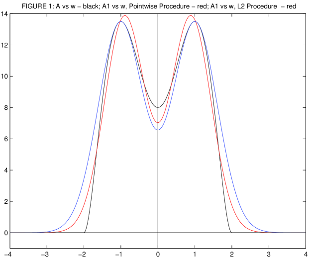
Figure 1: Comparison between pointwise and $L^{2}$ selection procedures with example (35)–(36): original signal $A$ is in black, pointwise algorithm in blue and $L^{2}$ in red.

The results for this simple example are not atypical of the general case; namely, one application of either selection process typically yields an approximation, $A_{p}(\cdot)$, which is qualitatively similar to the given amplitude, $A(\cdot)$, but may differ quantitatively from $A(\cdot)$. This defect may be overcome by repeated applications of the procedure.

4.2 Hierarchical Refinements of Selection Procedures

We assume we have already applied either the pointwise or $L^{2}$ selection procedures $n-1$ times and constructed the functions $A_{N_{k},k}(\cdot),\ 1\leq k\leq n-1$, each which are sums of $N_{k}$ Gaussians. We let

$$\forall\omega\in(-\Omega,\Omega),\qquad A_{n}(\omega)=A_{0}(\omega)-\sum^{n-1}_{k=1}A_{p_{k},k}(\omega),$$

where $\omega\mapsto A_{o}(\omega)$ is the original amplitude, previously denoted by $A(\cdot)$. As defined $A_{n}(\cdot)$ is even and rapidly decreasing as $|\omega|\rightarrow\infty$. The principal qualitative difference between $A_{n}(\cdot)$ and $A_{o}(\cdot)$ is that $A_{n}(\cdot)$ takes on both positive and negative values. For definiteness, we assume now that $\omega=0$ is a maximum of $A_{n}(\cdot)$ and that the typical structure of $A_{n}(\cdot)$ is as follows:

• there are exactly $q_{n}$ negative-valued, local minima of $A_{n}(\cdot)$ at points

  $$0<\underline{\Omega}^{n}_{1}<\underline{\Omega}^{n}_{2}<\ldots<\underline{\Omega}^{n}_{q_{n}}$$

  and each minima is non-degenerate;

• there are exactly $p_{n}$ positive-valued, local maxima of $A_{n}(\cdot)$ at points

  $$0<\overline{\Omega}^{n}_{1}<\overline{\Omega}^{n}_{2}<\ldots<\overline{\Omega}^{n}_{p_{n}}$$

  and each maxima is non-degenerate;

• the minima and maxima are not necessarily interlaced since $A_{n}(\cdot)$ may have positive valued local minima and negative valued local maxima.

Graphs of $A_{1}(\cdot)=A_{0}(\cdot)-A_{1,0}(\cdot)$ for the two selection procedures used in our previous example are shown in Figure 2.

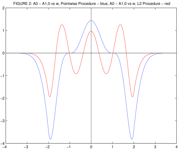
Figure 2: Difference $A_{0}(\omega)-A_{1,0}(\omega)$: pointwise selection in blue, $L^{2}$ selection in red.

Our induction step is to replace $A_{n}(\cdot)$ by a sum of $N_{n}=q_{n}+p_{n}+1$ even Gaussians:

$$\begin{array}[]{rcl}A_{N_{n},n}(\omega)&=&\alpha^{n}_{0}e^{-\frac{\omega^{2}}{2\overline{\sigma}_{0}^{n}}}+{\displaystyle\sum^{p_{n}}_{k=1}}\alpha^{n}_{k}\left(e^{-\frac{(\omega-\overline{\omega}^{n}_{k})^{2}}{2\overline{\sigma}^{n}_{k}}}+e^{-\frac{(\omega+\overline{\omega}^{n}_{k})^{2}}{2\overline{\sigma}^{n}_{k}}}\right)\\ &&-{\displaystyle\sum^{q_{n}}_{k=1}}\beta^{n}_{k}\left(e^{-\frac{(\omega-\underline{\omega}^{n}_{k})^{2}}{2\underline{\sigma}^{n}_{k}}}+e^{-\frac{(\omega+\underline{\omega}^{n}_{k})^{2}}{2\underline{\sigma}^{n}_{k}}}\right)\end{array}$$ (37)

where the $\alpha$’s, $\beta$’s, $\sigma$’s, and $\overline{\sigma}$’s are positive and the $\omega$’s and $\overline{\omega}$’s satisfy

$$0\leq\underline{\omega}^{n}_{1}<\underline{\omega}^{n}_{2}<\ldots<\underline{\omega}^{n}_{q_{n}},\qquad 0<\overline{\omega}^{n}_{1}<\overline{\omega}^{n}_{2}<\ldots<\overline{\omega}^{n}_{p_{n}}.$$

The pointwise selection procedure generates the unknown parameters by insisting that $A_{N_{n},n}(\cdot),\ A^{(1)}_{N_{n},n}(\cdot)$, and $A^{(2)}_{N_{n},n}(\cdot)$ match $A_{n}(\cdot),\ A^{(1)}_{n}(\cdot)$, and $A^{(2)}_{n}(\cdot)$ at the local maxima $\{0,\{\overline{\Omega}^{n}_{k}\}^{p_{n}}_{k=1}\}$ and local minima $\{\underline{\Omega}^{n}_{k}\}^{q_{n}}_{k=1}$. The $L^{2}$ selection procedure chooses the coefficients to minimize $||A_{n}(\cdot)-A_{N_{n},n}(\cdot)||^{2}$. This problem has the same structure as the optimization problem discussed in detail earlier, and may be solved by the “steepest-ascent” algorithm. The optimal solution satisfies

$$0\leq||A_{n+1}(\cdot)||^{2}=||A_{n}(\cdot)-A_{N_{n},n}(\cdot)||^{2}=||A_{n}(\cdot)||^{2}-Q_{n,{\rm max}},$$ (38)

where $(\underline{\omega}^{n},\underline{\sigma}^{n};\overline{\omega}^{n},\overline{\sigma}^{n})\rightarrow Q_{n}=||A_{N_{n,n}}(\cdot)||^{2}$ when the $\alpha$’s and $\beta$’s are the least squares parameters corresponding to the given choice $\underline{\omega}^{n},\underline{\sigma}^{n},\overline{\omega}^{n}$, $\overline{\sigma}^{n}$ and $Q_{n,{\rm max}}=\underset{(\underline{\omega}^{n},\underline{\sigma}^{n},\overline{\omega}^{n},\overline{\sigma}^{n})}{\rm max}Q_{n}$. The equality (38) implies that

$$0\leq||A_{n+1}(\cdot)||^{2}=||A_{0}(\cdot)-\sum^{n}_{j=0}A_{N_{j},j}(\cdot)||^{2}=||A_{0}(\cdot)||^{2}-\sum^{n}_{j=0}Q_{j,{\rm max}},$$

and provides us with a stopping criteria for the number of applications of the $L^{2}$ selection procedure. Specifically, we stop when $||A_{n+1}(\cdot)||^{2}\leq\epsilon_{\rm stop}$, a preassigned tolerance. The stopping criteria for the pointwise selection procedure is equally easy; we stop when

$$\underset{\omega}{\rm max}(A_{n+1}(\omega))\leq\epsilon_{\rm stop}\ \ {\rm and}\ \ \underset{\omega}{\rm min}(A_{n+1}(\omega))\geq-\epsilon_{\rm stop}.$$ (39)

Figures 3 and 4 shows the results of applying the hierarchical $L_{2}$ procedure 2,3, and 4 times, respectively. The “black” curves on each figure are the original amplitude, $A(\cdot)$, and the “red”curves are the composite hierarchial gaussian approximations. In applying the $L^{2}$ procedure twice we went from 1 to 5 even gaussians; in the third application we went from 5 to 16 even gaussians, and in the fourth application from 16 to 47 even gaussians. After four applications of the algorithm, the curves become indistinguishable.

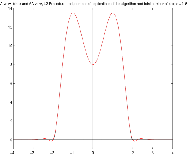
Figure 3: $L^{2}$ hierarchical refinement procedure (to be continued in Fig. 4): Original signal $A$ is in black and $L^{2}$ in red.

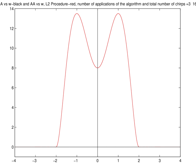
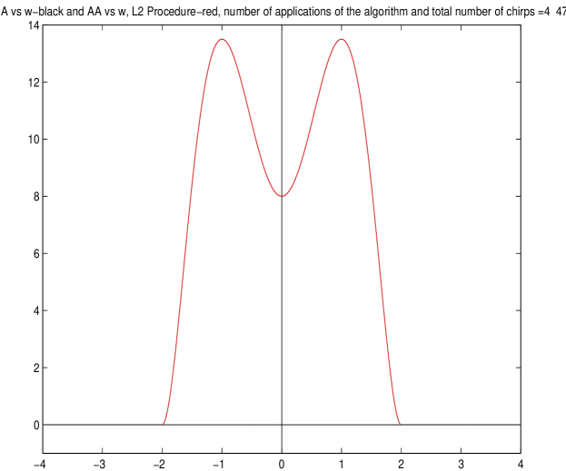
Figure 4: $L^{2}$ hierarchical refinement procedure, continued from Fig. 3.

5 Two “real-life” applications

5.1 Chirp decomposition of a noisy signal

A band-limited signal slightly corrupted by white noise isn’t band limited anymore; however, if we set up the preceding algorithms with a value of $\Omega$ being large enough, it may be possible to recover a correct approximation. First of all, we set up the following data: consider the even amplitude function displaying only two bumps,

$$A(\omega)=\frac{\exp(-a|\omega|^{3})-\exp(-b|\omega|^{3})}{b-a};\qquad a=0.8,\ b=1.3.$$ (40)

We couple it with different phase functions of increasing complexity: first, we chosed a cubic one, $\phi(\omega)=\frac{\omega^{3}}{50}$ and then $\phi(\omega)=\pi(1-\exp(-\omega^{2}))\sin(2\omega)$. The discretization grid is 512 points from $t=-5.1$ to $t=5.12$. We don’t insist on the fact that in case the original phase function $\phi$ is a polynomial of degree 2, its recovery is exact.

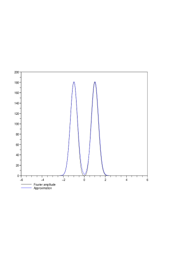
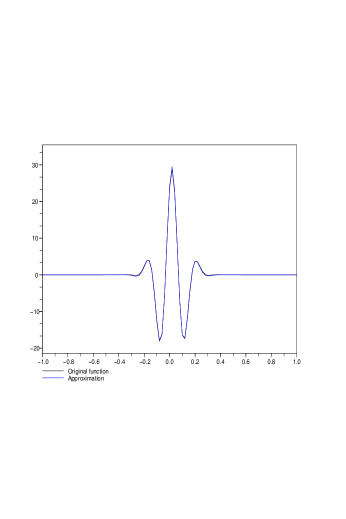
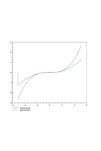
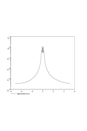
Figure 5: Pointwise procedure selection on example (40) for cubic phase.

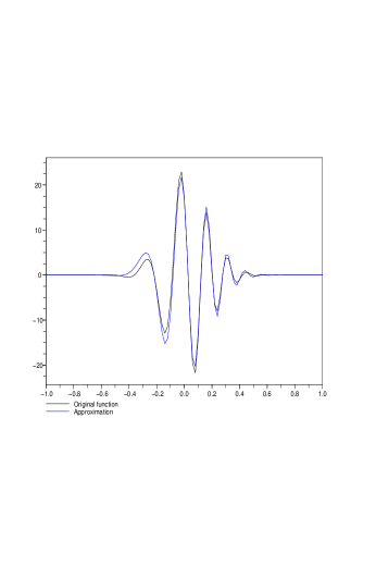
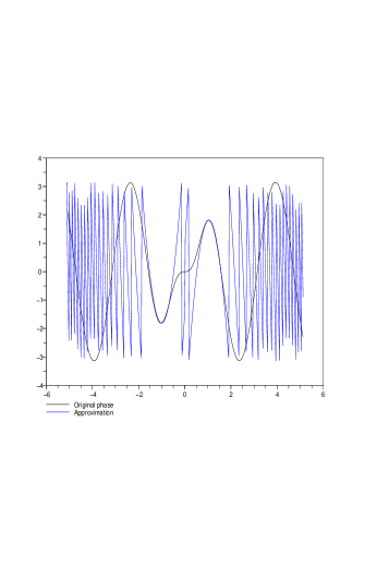
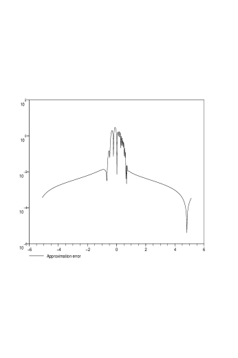
Figure 6: Pointwise procedure selection on example (40) for sinusoidal phase.

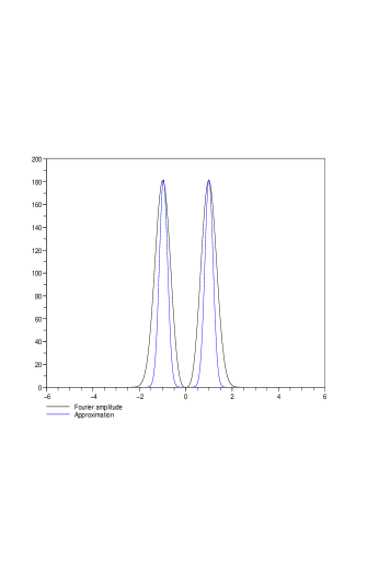
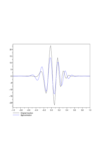
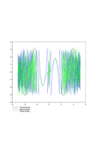
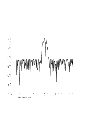
Figure 7: Pointwise procedure selection on example (40) slightly corrupted by white noise with sinusoidal phase.

The specificity of these runs is that now, we test the algorithm “blind”, which means that we just furnish the collection of sample data for both amplitude and phase, and we look after the maximum numerically. Similarly, the derivatives involved in the parameters calculation are computed with finite differences. Corresponding results are displayed in the Figures 5–7. On the left column, one sees the original amplitudes and phases (in black) and their approximations (in blue); on the right one, there are the signal as a function of $t$ (in black), its chirplet approximation (in blue) and finally the absolute error in log-scale. The recovery of the amplitude (40) by means of two Gaussians looks very satisfying and errors are noticeable only in the last example where the original signal is corrupted by white noise; the cubic phase (Fig. 5) is approximated in a correct way by second degree polynomials around the maxima of $A$ which are well identified. Of course, in case $A$ would display several local extrema, a more involved process would have to be set up in order to localize them properly inside the vector of samples. Concerning the sinusoidal phase model (Fig. 6), its recovery by means of polynomials of degree two is of course rather poor; however, what really matters is that it is correct in the vicinity of maximum points of $A$, and this is just what happens (see [16]). The behavior of these approximations in the $t$ variable is good, and the absolute error remains reasonable.

Fig. 7 deals with a more difficult test-case, namely we set up the amplitude (40) with the sinusoidal phase, we perform the inverse Fourier transform to get it as a function of $t$, we corrupt the resulting signal with white noise (which makes it not band-limited anymore). This is the data we furnish to the algorithm of §3.1. Obviously, the white noise has to remain small in order not to perturb the maxima of $A$. What we found is that even this requirement isn’t enough as the phase function should not be corrupted too much in order to let the algorithm approximate it locally by a parabola correctly. In this case, the absolute recovery error is bigger compared to the noise-free case (see again Fig. 6).

5.2 Finding chirp patterns in stock market indices

The Hang-Seng Composite Enterprise Index is one of the main index for the Chinese stock market and the CAC 40 is the leading index for the Parisian place. We used the corresponding daily price fluctuations on an interval of 1024 days (ending on august 29th 2008) in order to check on a real-life case whether or not the level of tolerance to noise was acceptable. Clearly, in order to avoid as much as possible spurious local extrema in the Fourier spectrum of the data, we detrended the prices by a global least-squares interpolation; polynomials of degree 5 and 6 have been used. Moreover, for the CAC 40 only, the detrended fluctuation was displaying quite a sharp peak corresponding to a periodic cycle. We also used a Basis Pursuit algorithm to remove as much as possible the white noise components of these fluctuations, see [3].

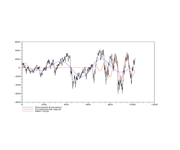
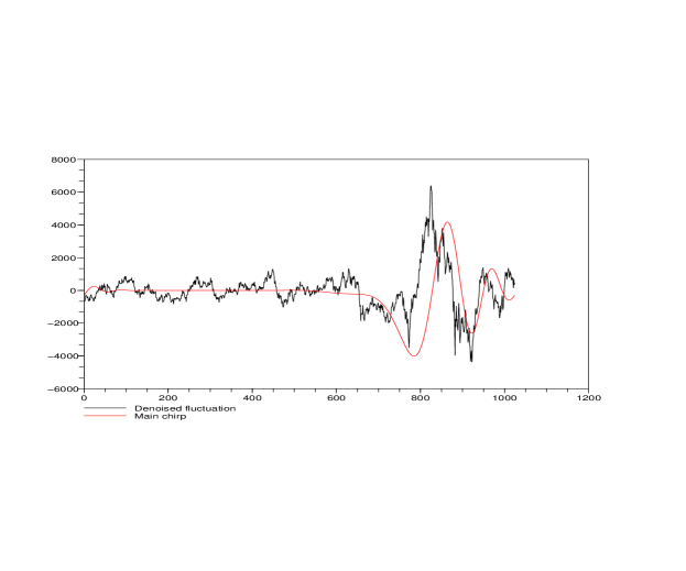
Figure 8: Chirp patterns in the daily price fluctuations of CAC 40 (top) and HSCEI (bottom).

On Fig. 8, we display the detrended data (in black), the long-lasting periodic cycle of the CAC 40 (in blue) and the chirps we got out of the algorithm of §3.1. The case of the Chinese index seem to be quite interesting as the recovery seems to be quite sharp. Results on both CAC 40 and HSCEI suggest that a qualitative change in the behavior of blue chips quotations occurred after the ignition of the so-called subprime crisis/credit crunch (corresponding to abscissa $t\simeq 700$).

References

- [1] A. Bultan, “A four-parameter atomic decomposition of chirplets,” IEEE Transactions on Signal Processing, vol. 47, pp. 731-745, March 1999.
- [2] E. Candès, P.R. Charlton, H. Helgason, “Detecting highly oscillatory signals by chirplet path pursuit”, Applied and Computational Harmonic Anal. vol. 24, pp. 14–40 (2008).
- [3] S. Shaobing Chen, D.L. Donoho, M.A. Saunders, “Atomic decomposition by basis pursuit”, SIAM J. Sci. Comput., vol. 20, pp. 33-61 (1998).
- [4] B. Dugnol, G. Fernandez, G. Galiano, J. Velasco, “On a chirplet transform-based method applied to separating and counting wolf howls”’, Signal Processing vol. 88 (July 2008) pp. 1817-1826.
- [5] G.B. Folland and A. Sitaram, “The uncertainty principle: a mathematical survey”, J. Fourier Anal. & Applic., vol. 3 (1997), 207-238.
- [6] J.M. Greenberg, Z. Wang, and J. Li, “New Approaches for Chirplet Approximations”, IEEE Transactions on Signal Transactions, to appear.
- [7] R. Gribonval, “Fast ridge pursuit with multiscale dictionary of gaussian chirps,” IEEE Transactions on Signal Processing, vol. 49, pp. 994-1001, May 2001.
- [8] C.J. Kicey and C.J. Lennard, “Unique reconstruction of band-limited signals by a Mallat-Zhong wavelet transform algorithm”, J. Fourier Anal. & Applic., Vol. 3, pp. 63-82, janvier 1997
- [9] H. Kwok and D. Jones, “Improved FM demodulation in a fading environment,” Proc. IEEE Conf. Time-Freq. and Time-Scale Anal., pp. 9-12, February 1996.
- [10] J. Li and P. Stoica, “Efficient mixed-spectrum estimation with applications to target feature extraction,” IEEE Transactions on Signal Processing, vol. 44, pp. 281-295, February 1996.
- [11] J. Li, D. Zheng, and P. Stoica, “Angle and waveform estimation via RELAX,” IEEE Transactions on Aerospace and Electronic Systems, vol. 33, pp. 1077-1087. July 1977.
- [12] S. Mallat and Z. Zhong, “Matching pursuit with time-frequency dictionaries,” IEEE Transactions on Signal Processing, vol. 41, pp. 3397-3415, December 1993.
- [13] S. Mann and S. Haykin, “The chirplet transform: physical considerations,” IEEE Transactions on Signal Processing, vol. 43, pp. 2745-2761, November 1995.
- [14] J.C. O’Neill and P. Flandrin, “Chirp hunting,” Proc. IEEE Int. Symp. on Time-Frequency and Time-Scale Analysis, pp. 425-428, October 1998.
- [15] A. Olevskii, A. Ulanovskii, “Universal Sampling and Interpolation of Band-limited Signals”, Geometric And Functional Analysis, to appear
- [16] A. V. Openheim and J. S. Lim. “The importance of phase in signals”. Proceedings of the IEEE, vol. 69 pp. 529-541, 1981
- [17] W. Rudin “Analyse réelle et complexe” (chapter 19). Masson éditeur, 1975
- [18] Th. Strohmer, “On Discrete Band-limited Signal Extrapolation”, Contemp. Math. 190:323-337 (1995).
- [19] Q. Yin, H. Qian, A. Feng, “A fast refinement for adaptive Gaussian chirplet decomposition”, IEEE Trans. on Signal Processing vol. 50, 2002, pp. 1298-1306