An Inexpensive Field-Widened Monolithic Michelson Interferometer for Precision Radial Velocity Measurements

Abstract

We have constructed a thermally compensated field-widened monolithic Michelson interferometer that can be used with a medium-resolution spectrograph to measure precise Doppler radial velocities of stars. Our prototype monolithic fixed-delay interferometer is constructed with off-the-shelf components and assembled using a hydrolysis bonding technique. We installed and tested this interferometer in the Exoplanet Tracker (ET) instrument at the Kitt Peak 2.1m telescope, an instrument built to demonstrate the principles of dispersed fixed delay interferometry. An iodine cell allows the interferometer drift to be accurately calibrated, relaxing the stability requirements on the interferometer itself. When using our monolithic interferometer, the ET instrument has no moving parts (except the iodine cell), greatly simplifying its operation. We demonstrate differential radial velocity precision of a few m s^-1 on well known radial velocity standards and planet bearing stars when using this interferometer. Such monolithic interferometers will make it possible to build relatively inexpensive instruments that are easy to operate and capable of precision radial velocity measurements. A larger multi-object version of the Exoplanet Tracker will be used to conduct a large scale survey for planetary systems as part of the Sloan Digital Sky Survey III (SDSS III). Variants of the techniques and principles discussed in this paper can be directly applied to build large monolithic interferometers for such applications, enabling the construction of instruments capable of efficiently observing many stars simultaneously at high velocity-precision.

1. INTRODUCTION

Since the discoveries of the first extrasolar planets (Wolszczan & Frail, 1992; Mayor & Queloz, 1995) more than 290 planets have been discovered using radial velocity techniques, transit searches, and microlensing. The majority of the known extrasolar planets have been discovered using precision radial velocity measurements that detect the gravitational influence of the planet on the parent star. The presence of the planet induces a periodic change in the line of sight velocity of the star and this velocity is measured using the small Doppler shift in the spectral lines of the star. Ongoing radial velocity surveys with high resolution echelle spectrographs have achieved velocity precisions of $1-3$ m s^-1 (Butler et al., 1996; Rupprecht et al., 2004), allowing the detection of $m\sin{i}=7-20$ Earth mass planets close to their host star (Santos et al., 2004; Rivera et al., 2005). These echelle spectrographs are generally large and expensive instruments which are not easily duplicated, leading to the availability of such instruments becoming a limiting factor in intensifying high-precision radial velocity surveys. High precision radial velocity observations of more stars are necessary in order to discover lower mass planets, explore different regimes of stellar mass and evolution (Johnson et al. 2007), planet formation around young stars (Setiawan et al. 2007), and to discover more planets around low-mass M stars (e.g. Endl et al. 2007).

Over the past few years we have developed the dispersed fixed-delay interferometer (DFDI) technique (Erskine & Ge, 2000; Ge, 2002; Ge, Erskine, & Rushford, 2002) into viable instruments capable of achieving high precision radial velocity measurements on stars and detecting extrasolar planets. Such instruments are substantially less expensive than echelle spectrographs since they do not require high spectral resolutions or large-format gratings. At the heart of these instruments is a stable, field-widened, fixed-delay Michelson interferometer. One such instrument, the Exoplanet Tracker (ET) instrument at the Kitt Peak 2.1m has been used to confirm known exoplanets (van Eyken et al. 2004) and detect a hot Jupiter around HD102195 (Ge et al. 2006). The ability to reliably construct monolithic Michelson interferometers has the potential to make such instruments stable, easy to use, and relatively easy to duplicate. This will enable multiple versions of these instruments to easily be built to complement existing echelle spectrographs in order to meet the need for high precision radial velocity measurements to support upcoming space missions like KEPLER (Borucki et al. 2003) and SIM (Shao et al. 2007). An additional advantage of the DFDI technique is the ability to observe a large number of stars simultaneously using a wide field-of-view telescope. This technique will be utilized to conduct MARVELS (Multi-object Apache point observatory Radial Velocity Exoplanet Large-area Survey), a multi-object survey for exoplanets, as part of SDSS III (Ge et al. 2007). MARVELS will be able to simultaneously monitor 120 F,G, and K stars in the 3 degree field of view of the Sloan 2.5m telescope, efficiently searching for Jupiter-mass planets (Ge et al., 2007).

The Michelson interferometer is a crucial component of the ET and MARVELS instruments and needs to be stable in order to reliably recover relative velocity drifts of a few m s^-1. Phase drifts of the interferometer during an exposure will tend to wash out the fringes, reducing the measured fringe visibility and the velocity precision. Large drifts between observing runs make it difficult to achieve coherent velocity links over large timespans. The current Michelson interferometer setup for the ET instrument at Kitt Peak uses a piezoelectric transducer (PZT) to control the path difference. This stabilizes the interferometer fringe and reduces the interferometer fringe phase drifts. The need to run a closed-loop system on the most critical component also makes observations difficult, since the observer has to continually monitor the phase, and restart the PZT after a software or computer failure. In terms of a long duration survey for exoplanets, failure of the PZT can lead to the inability to coherently link radial velocities. The PZT control also becomes increasingly more difficult for multi-object instruments based on ET that use much larger beamsplitters due to the need to accommodate more fibers.

To address some of these problems and to make ET-like instruments more stable and substantially easier to use, we have been pursuing a program to design and build an inexpensive monolithic interferometer that satisfies our criteria of field widening and stability (see Mahadevan et al. 2004). Monolithic interferometers have also been discussed by Mosser et al. (2007) for use in asteroseismology from DOME C in Antarctica. Polarizing Michelson interferometers similar to our prototype have been in use for solar oscillation measurements for a number of years in the Global Oscillation Network Group (GONG, Harvey et al. 1995) and Solar and Heliospheric Observatory Michelson Doppler Imager (SOHO MDI) instruments and are the design chosen for the Helioseismic and Magnetic Imager (HMI) instrument (Graham et al. 2003) on the planned Solar Dynamics Observatory. Monolithic interferometer assemblies have also been used to measure the solar resonance fluorescence of OH (Englert et al. 2007). Polarizing interferometers are usually designed to observe a single absorption line, while interferometers built for spatial heterodyne spectroscopy are only effective over a small wavelength region. The monolithic interferometer for the ET instrument needs to be able to function in the wavelength range 5000-6000 Å, be non-polarizing, and have a slight tilt in one mirror to created the fringes observed with ET.

In this paper we describe the construction of an inexpensive prototype monolithic interferometer and present results demonstrating the ability to acquire precise stellar radial velocities using the monolithic interferometer with the Exoplanet Tracker (ET) instrument.

2. Fixed Delay Interferometers: History and Background

By the term fixed-delay interferometer we refer to interferometers that operate in a narrow range of delays (usually a few $\mu$m change in path length) unlike the interferometers used in Fourier transform spectrographs which need to be scanned over large path lengths. Fixed-delay interferometers and interferometers coupled to spectrographs have often been used to aid calibration and enable precise wavelength and velocity measurements. Fabry-Perot interferometers have been used with spectrographs to measure precise radial velocities of stars (McMillan et al. 1994; Connes et al. 1996) by using them to track and calibrate out instrument drifts. Fixed-delay interferometers are also routinely used for high precision velocity measurements of solar oscillations (Gorskii & Lebedev 1977; Beckers & Brown 1978; Kozhevatov 1983; Harvey et al 1995 and Graham et al. 2003). Their use has also been proposed to detect stellar oscillations and oscillations of Jupiter (Forrest et al. 1978; Mosser et al. 1998; Mosser et al. 2003).

For an interferometer with an optical path difference $d$:

$$m\lambda=d$$ (1)

where $m$ is the fringe order and $\lambda$ the monochromatic wavelength of interest. A small change in the wavelength due to a Doppler shift will also change the fringe order since the interferometer delay ($d$) remains the same if the interferometer is stable.

$$\Delta m=\frac{d}{\lambda^{2}}\Delta\lambda$$ (2)

Using the Doppler shift formula for non-relativistic velocities

$$\frac{\Delta\lambda}{\lambda}=\frac{\Delta v}{c}$$ (3)

we can write Equation 2 as

$$\Delta m=\frac{d}{\lambda}\frac{\Delta v}{c}$$ (4)

$$\Delta v=\frac{c\lambda}{2\pi d}\Delta\phi$$ (5)

where $\phi=2\pi m$ is the phase of the interference order. A change in velocity causes a Doppler shift in the wavelength of the light. This Doppler shift can be measured from the phase shift ($\Delta\phi$) if the interferometer delay ($d$) is known. The phase and phase shift can be measured either by stepping the interferometer through small changes in the optical delay, or by putting a small tilt on one interferometer mirror so that the phase can be measured in a single exposure using a two dimensional image.

Figure 1 illustrates the phase pattern for a monochromatic emission line. The phase pattern shown is for a collimated beam passing through a field-widened Michelson interferometer that has a slight tilt on one mirror. A change in the wavelength of the incident light leads to a shift in phase of the output fringe pattern from the interferometer. The velocity shift can then be estimated using Equation 5 since the shift in phase of the sinusoidal pattern can be easily measured. This ability to measure phase shifts is also applicable for a narrow wavelength band containing a single absorption line (Harvey et al. 1995). Real stellar spectra, however, have thousands of stellar lines and using the largest possible number of lines will yield the best velocity precision. A large wavelength range of light passing through the interferometer will lead to a dramatic reduction of the recorded fringe visibility since different wavelengths will have different phase shifts in the output pattern. Almost no interference fringes will be visible in the output phase pattern, making the estimation of phase shifts and velocity very difficult. Using an interferometer alone one can achieve good velocity precision on bright sources, but the use of only a single absorption line, or a small wavelength region, makes it difficult to obtain the velocity accuracy required to detect planets around stars due to the limited number of photons collected.

In 1997 David Erskine (then at Lawrence Livermore National Labs) proposed using a field-widened Michelson interferometer in series with a medium resolution spectrograph for the measurement of precise radial velocities. The spectrograph is used to disperse the light, allowing the measurement of fringe visibilities over a significantly wider wavelength range. The first results from such an instrument are found in Erskine & Ge (2000) and Ge et al. (2002), and the theoretical basis for the use of such an instrument is outlined in Ge (2002), Erskine et al. (2003) and Mosser et al. (2003). Figure 2 shows a simulation of the spectral format expected from a dispersed fixed-delay interferometer instrument. The interferometer fringes are clearly visible due to dispersion by the medium-resolution spectrograph. The normalized fringe pattern ($I$) in the slit direction for each wavelength channel can be expressed in terms of velocity using Equation 5

$$I=1+\gamma\sin{(2\pi d\frac{\Delta v}{c\lambda}+\phi_{0}})$$ (6)

where $\phi_{0}$ is the phase of the first pixel and $\gamma$ is the fringe visibility defined using the maximum ($I_{max}$) and minimum ($I_{min}$) intensities of the sinusoidal fringe pattern

$$\gamma=\frac{I_{max}-I_{min}}{I_{max}+I_{min}}$$ (7)

A Doppler velocity shift of the absorption line manifests itself as a phase shift of this sinusoidal pattern. The accuracy with which the radial velocity can be measured from one fringe is related to the photon noise error and the fringe visibility ($\gamma$) and is discussed in §4.2.

3. The Current Exoplanet Tracker Instrument

The current Exoplanet Tracker (ET) instrument at Kitt Peak is the end product of many years of experimentation with various design ideas for high throughput DFDI instruments. ET has been built to enable precision radial velocity measurements on slowly rotating main sequence stars, and the exoplanet HD102195b was discovered using radial velocities obtained with this instrument (Ge et al. 2006). Aspects of the instrument design have been mentioned in van Eyken et al (2003, 2004), Ge et al. (2003, 2004, 2006), and Mahadevan et al. (2004, 2008). In this section we briefly review the design aspects of the instrument that are relevant from the point of view of installing and testing a prototype monolithic interferometer. Figure 3 shows the optical layout of the KPNO ET instrument. Relevant components are described below.

3.1. Optical Fibers and Fiber Feed

The optical fibers and fiber feed used in ET are inherited from the Fiber Optic Echelle instrument (Ramsey & Huenemoerder 1986). The efficiency and properties of these optical fibers are described in Barden (1998). Each fiber cable is enclosed in a flexible metal covering and is 22 meters in length. The optical fiber used in the ET instrument is a $200$ $\mu$m high $OH$ fiber. In the f/8 beam of the telescope this fiber subtends an angle of $\sim 2.5$ arc seconds on the sky. The use of the optical fiber enables the ET instrument to be mechanically de-linked from the telescope and in an isolated enclosure with very few moving parts. This allows the instrument environment to be well controlled and eliminates mechanical flexure due to movement, minimizing velocity drifts that need to be calibrated out. The ET instrument can be used with either the 2.1m telescope or the 0.9m Coudé telescope simply by switching the 200$\mu$m optical fiber from one telescope to another. The scrambling properties of the optical fiber (Heacox 1986, Hunter  Ramsey 1991) make the illumination of the Michelson interferometer and spectrograph slit much more uniform.

3.2. Instrument Location and Enclosure

The ET instrument is currently installed in a small insulated room within the coudé spectrograph room at the base of the 2.1m telescope dome. The spectrograph room is very stable and its temperature only responds slowly to the outside temperature. The instrument itself is built on a vibration isolated optical table. A baseboard heater is installed at one end of the room and a thermostat at the other end senses the ambient temperature of the air and controls the heater. A secondary enclosure made of insulating panels is built on the optical table to further reduce the effect of temperature variations and to minimize the turbulence. Figure 4 shows the temperature of the ET instrument measured at four locations. The temperature of the instrument within the inner instrument enclosure is more stable than the temperature of the room itself.

3.3. Iodine Cell

An iodine cell manufactured by Triad Technologies is used in the ET instrument to provide a simultaneous calibration of the instrument drift. A motor allows the iodine cell to be inserted or removed from the collimated stellar beam path. The cell is operated at a temperature of $60\pm 0.1^{\circ}$C. The dense absorption spectra of $I_{2}$ are superimposed on the stellar absorption lines. Since the starlight passes through the iodine cell, the two intermingled spectra experience exactly the same illumination in the interferometer and spectrograph, and therefore track the same instrument drifts.

3.4. Input Optics and Michelson Interferometer

The ET input optics are designed to account for the focal ratio degradation of the 200$\mu$m optical fiber and able to collect most of the photons exiting the fiber. The output beam from the fiber is collimated to a diameter of $\sim 6.6$ mm and passes through the iodine cell if the cell is inserted into the beam path. A cylindrical lens then collapses the beam in one direction (dispersion, or horizontal direction) and the beam is focused onto the mirrors of the Michelson interferometer. The Michelson interferometer used in ET has a 4 mm BK7 glass etalon in one arm, an air-gap in the other and is designed to have an optical delay of $\sim 7$ mm. The lengths of the two arms are also chosen so that the interferometer optical delay is relatively insensitive to the angle of the converging beam from the cylindrical lens. This ‘field widening’ of the interferometer is described in more detail in §4.3. A small tilt in one beam of the interferometer allows the creation of $3-4$ horizontal fringes over the 6.6 mm stellar beam. A slight tilt of the interferometer beam cube allows both the transmitted and reflected beams to be imaged onto the spectrograph slit using relay mirrors.

3.5. Piezoelectric Transducer for Interferometer Stabilization

We use a piezoelectric transducer (PZT) to keep the interferometer from drifting during an exposure (drifts lead to decreased fringe visbility) and keep the delay stable. Piezoelectric materials can generate mechanical stress in response to applied electric voltage, enabling the interferometer delay to be maintained even in the presence of vibration and temperature drifts. The PZT is attached to one of the interferometer mirrors and is controlled using a LabView program. A single-mode fiber fed with a stabilized He-Ne laser (632.8 nm) is used to illuminate a small portion of the beam splitter. The horizontal fringes formed are recorded by a video camera and are used as the input to the LabView program. The position of these fringes is then locked by applying the appropriate voltages to the PZT. This method can effectively stabilize the interferometer fringe pattern over the period of an observing run ($7-12$ days). To obtain flats and calibration lamp spectra the PZT voltage is ramped very quickly, leading to the PZT mirror vibrating and washing out the interference fringes. The PZT is turned off after every observing run, re-initialized and dialed back to its previous position at the start of a new observing run.

3.6. Spectrograph

The ET spectrograph is a transmissive design with an f/5 collimator, a volume phase holographic transmission grating and a $\sim f/2$ camera. The spectrograph optics were designed by Dequing Ren. The stellar beam from the interferometer is imaged on the spectrograph slit and collimated. Unlike normal spectrographs, where the starlight is brought to a focus at the slit, the ET slit is not at the point where the beam is smallest but where its fringe visibility is maximal. The pre-slit optics form an image of one of the interferometer mirrors onto the slit, and change the slow beam to an f/5 beam. The spectrograph then disperses the light, forming an image of the slit (and the interference fringes) on the detector.

3.7. Spectral Format & Efficiency

The ET instrument operates in the grating first order, but its spectral format is two dimensional to allow the measurement of the fringe phase at each wavelength. The $250$ $\mu$m slit is sampled by 6.7 pixels on the detector, yielding a spectral resolution of $\sim 6000$. The fringes in the slit direction are sampled by $\sim 58$ pixels. Figure 5 shows the spectral format of the instrument. The top and middle spectra are the two outputs from the interferometer. The measured instrument efficiency from the fiber output to the detector plane is $\sim 49\%$. This efficiency includes losses from the lenses, mirrors, interferometer, slit and the grating, but not the iodine cell or the CCD. The CCD is expected to have a quantum efficiency of $\sim 90\%$ in our wavelength range. Using the measured fiber and telescope transmission in average seeing, and assuming their efficiency to be 35-40$\%$ in average seeing the total instrument efficiency is calculated to be $\sim$ 15.5 – 17.5 %. The instrument efficiency in good seeing condition, measured using a flux calibration star, is $\sim 18\%$ and in good agreement with the expected values.

4. A Monolithic Michelson Interferometer for ET

A monolithic interferometer for an instrument like ET has a number of requirements in terms of delay, field widening and stability. In this section we explore these parameters and the materials that can be used in the construction of a monolithic interferometer.

4.1. The Choice of Optical Delay

The spectral format of ET allows one to measure the phase shift of the interference pattern and convert that to velocity. As outlined in Butler et al. (1996) and Ge (2002), the velocity uncertainty from one pixel of the normalized fringe is:

$$\sigma_{RMS}=<\frac{\epsilon_{I}}{dI/dv}>$$ (8)

The uncertainty in the measured intensity, $\epsilon_{I}$, is just the inverse of the signal to noise ratio (S/N^-1) if the S/N is large enough to ignore the dark current and read noise from the detector, a condition that always needs to be satisfied to achieve high-precision radial velocities with ET. For the sinusoidal interferometer fringes observed with ET:

$$<\frac{dI}{dv}>=\frac{\sqrt{2}\pi d\gamma}{c\lambda}$$ (9)

The radial velocity error from measurements of one fringe is then given by

$$\sigma_{RMS}=\frac{c\lambda}{\sqrt{2}\pi d\gamma\sqrt{N_{photons}}}$$ (10)

where $N_{photons}$ is the total number of photons recorded for all the pixels in the interferometer fringe. The functional form of this equation means that the highest velocity precision for a given number of photons is obtained when the value of $d\gamma$ is maximized. The value of the interferometer delay that yields the largest $d\times\gamma$ for a given wavelength region is, however, a function of the spectral type and the rotational velocity of the star. Since the interferometer effectively heterodynes information to lower spatial frequencies (Erskine et al. 2003), a fast rotator has less high frequency information and requires a smaller delay.

Figure 6 shows the $d\gamma$ at different optical delays ($d$) for a K5V star at various rotational velocities. These results are derived from simulations of the ET instrument spectral format using stellar models as an input. The chosen delay for the ET instrument is $\sim 7$ mm since this value provides adequate fringe visibility ($\gamma$) for late F, G and K stars that have $0<v\sin{i}<12$ km s^-1. Fast rotators (e.g. the planet bearing star Tau Boo) have very low fringe visibility at our chosen interferometer delay, making precise radial velocities difficult to extract. The optical delay of the interferometer does not need to be exact for our application, It merely needs to be stable. More detailed discussions regarding the calculation of optimal delay for different spectral parameters can be found in Mosser et al. (2003).

4.2. The Field Compensation Principle

The optical delay of a Michelson interferometer is strongly dependant on the incident angle of the light. Deliberately designing an interferometer to decrease this dependence of the optical delay on the incident angle is known as field widening, or field compensation, and is described in more detail in Hillard & Sheperd (1966), Shepherd et al. (1985), and Thullier & Sheperd (1985). A Michelson interferometer for ET must have arms of different lengths to create a total optical delay of $\sim 7$ mm, i.e., $\sim 14000$ waves of delay at a wavelength of 5000 Å. This delay is appropriate for observations of stars with $v\sin{i}<12$ km s^-1. For an interferometer with arm lengths $L_{1}$ and $L_{2}$, with refractive indices $n_{1}$ and $n_{2}$ respectively, the interferometer optical delay for an on-axis ray ($d_{0}$) is given by

$$d_{0}=2(n_{1}L_{1}-n_{2}L_{2})$$ (11)

For a ray entering the Michelson interferometer at an angle $i$ the interferometer delay can be written as (Shepherd et al. 1985)

$$d=2[n_{1}L_{1}(1-\frac{\sin^{2}i}{n_{1}^{2}})^{-\frac{1}{2}}-n_{2}L_{2}(1-\frac{\sin^{2}i}{n_{2}^{2}})^{-\frac{1}{2}}]$$ (12)

Expanding all terms of $\sin{i}$ upto fourth order and ignoring higher order terms we get

$$d=2[(n_{1}L_{1}-n_{2}L_{2})-\frac{\sin^{2}i}{2}(\frac{L_{1}}{n_{1}}-\frac{L_{2}}{n_{2}})-\frac{\sin^{4}i}{8}(\frac{L_{1}}{{n_{1}}^{3}}-\frac{L_{2}}{{n_{2}}^{3}})]$$ (13)

If the same material is used in both arms of the interferometer ($n_{1}=n_{2}$) the interferometer delay can be quite sensitive to the angle of the incident light. Such an interferometer is often referred to as an uncompensated interferometer. For example, an interferometer with air gaps in both arms and a 7 mm delay (at 5000 Å) has 19.1 waves of phase change over a 3 degree half-angle and 4.5 waves over a 1.5 degree half angle. Such large phase changes are unacceptable with the ET instrument since the fringe visibilities will be substantially reduced when the fringes are imaged on the slit.

The $\sin^{2}{i}$ term in Equation 13 for the delay disappears when

$$\frac{L_{1}}{n_{1}}=\frac{L_{2}}{n_{2}}$$ (14)

The delay for a compensated Michelson interferometer (ie. one that satisfies Equation 14) is then given by:

$$d=d_{0}[1+\frac{\sin^{4}i}{8{n_{1}}^{2}{n_{2}}^{2}}]$$ (15)

where $d_{0}$ is the interferometer delay when $i=0$, ie. when the ray is along the axis of the interferometer. For small values of $i$ the delay is almost independent of the incident angle. Further increase in field widening (so called super field widening) can be achieved by using two or more glasses with an air space to also reduce the effect of the $\sin^{4}{i}$ term (eg. Gault, Johnston & Kendall 1985), but we have not attempted this for our prototype monolithic interferometer.

Any field compensated Michelson interferometer at a specific delay must therefore simultaneously satisfy Equations 11 and 14. The complete disappearance of the $\sin^{2}{i}$ term in Equation 13 can only be achieved for a specific design wavelength (5000 Å in this case). The simplest choice for the ET interferometer was to use the same material as the beamspliiter (BK7) in one arm and an air-gap in the other. To find the values of $L_{1}$ and $L_{2}$ that satisfy our constraints we calculate the refractive index of BK7 at the design wavelength using the Sellmeier dispersion formula. The dispersion constants used in this equation may vary slightly depending on the glass melt and the values we use are for typical melts of N-BK7. The values of the arm lengths that satisfy the field widening condition are $L_{1}$(BK7) = 4.04 mm and $L_{2}$(air) = 2.66 mm. The wavelength dependence of the refractive index and errors in the dimensions of the arms will, in reality, lead to a situation where the compensation condition is not met exactly. To evaluate the performance in such a case we define a term $\epsilon$ which is a wavelength dependant measure of the departure from the field widening condition.

$$\epsilon=\frac{L_{1}}{n_{1}}-\frac{L_{2}}{n_{2}}$$ (16)

Even when $\epsilon=0$ at 5000 Å the variation of refractive index with wavelength results in a non-zero value of $\epsilon$ creating a small dependence of the delay on the $\sin^{2}{i}$ term for wavelengths other than 5000 Å. The phase difference caused by this effect at the calculated values of $L_{1}$ and $L_{2}$ is illustrated in Figure 7 for a beam with a half-angle of 1.5 degrees. Although the ET instrument only works in the 5000-5600 Å region, such an interferometer can, in principle, be used over wider wavelength regions, and we have calculated the phase difference for 4000-6000 Å which is the spectral range containing most of the radial velocity information for F, G, K stars (Bouchy et al., 2001). For a hypothetical case in which the compensation condition is off by $\epsilon=100$ $\mu m$ even at 5000 Å , a phase shift of 0.137 waves occurs for a beam with a half angle of 1.5 degrees. This will lead to a slight decrease in the observed visibility, but is otherwise acceptable as long as the focal ratio or the illumination pattern of the beam does not change significantly. If an iodine cell is used in the beam path, then small changes in the illumination do not matter since the iodine and starlight are both affected in the same way. The scrambling properties of the optical fibers used in ET also ensure that the illumination of the interferometer is stable even in bad seeing conditions.

4.3. Reducing Sensitivity to Temperature Drifts

The need for a particular value of the optical delay and field compensation fixes the values of the arm lengths $L_{1}$ and $L_{2}$ since we have decided to use BK7 glass in one arm and an air-space in the other. However, since our goal is to build a stand alone monolithic interferometer, whose arms are isolated from any external mechanical mounts, the choice of spacer material for the air arm still needs to be made. The delay for a beam going through a compensated Michelson interferometer with a very small angle of inclination is shown in Equation 11. Following Title & Ramsey (1980), variation of the interferometer phase with temperature can then be written as

$$\frac{d(d_{0})}{dT}=2(n_{1}\frac{dL_{1}}{dT}+L_{1}\frac{dn_{1}}{dT}-n_{2}\frac{dL_{2}}{dT}-L_{2}\frac{dn_{2}}{dT})$$ (17)

Using the field widening condition (Equation 14) the right hand side of this equation can be recast in the form

$$2\frac{L_{1}}{n_{1}}({n_{1}}^{2}(\frac{1}{n_{1}}\frac{dn_{1}}{dT}+\frac{1}{L_{1}}\frac{dL_{1}}{dT})-{n_{2}}^{2}(\frac{1}{n_{2}}\frac{dn_{2}}{dT}+\frac{1}{L_{2}}\frac{dL_{2}}{dT}))$$ (18)

which disappears when

$${n_{1}}^{2}(\frac{1}{n_{1}}\frac{dn_{1}}{dT}+\frac{1}{L_{1}}\frac{dL_{1}}{dT})={n_{2}}^{2}(\frac{1}{n_{2}}\frac{dn_{2}}{dT}+\frac{1}{L_{2}}\frac{dL_{2}}{dT})$$ (19)

This thermal compensation condition depends only on the refractive indices, their variation with temperature, and the linear thermal expansion coefficients of the materials used, and is independent of the actual arm lengths or path differences. In our case the left-hand-side of the equation is already predetermined by the choice of BK7 as the material in that arm. A wise choice of spacer material for the other arm can then be used to athermalize the interferometer. To evaluate the variation of refractive index with temperature of BK7 we use the equation

$$\frac{dn_{abs}}{dT}=\frac{n^{2}(\lambda,T_{0})-1}{2n(\lambda,T_{0})}(D_{0}+2D_{1}\Delta T+3D_{2}{\Delta T}^{2}+\frac{E_{0}+2E_{1}\Delta T}{\lambda^{2}-\lambda_{TK^{2}}})$$ (20)

where $\lambda$ is the wavelength of interest, $\Delta T$ is the temperature difference from the reference temperature $T_{0}$ ($20^{\circ}$ C) and $n$ is the refractive index for that wavelength calculated at the reference temperature using the Sellmeier dispersion formula. Using this equation, the variation of refractive index of BK7 with temperature can be calculated with constants ($D_{0}-D_{2},E_{0},E_{1}$) provided in the Schott optical glass catalog. Using Equation 18 and assuming vacuum operation, the change in delay and the velocity drift can be estimated for various materials. Using Equation 5, the shift of one fringe ($2\pi$ in phase) corresponds to a velocity shift of

$$\Delta v=\frac{c\lambda}{d_{0}}$$ (21)

For our value of $d_{0}\sim 7$ mm, one fringe shift corresponds to a velocity shift of $\sim 21.5$ km s^-1. Table 1 shows the velocity shift for a one degree change in temperature using BK7, copper, CaF₂, or aluminium as a spacer material for an interferometer operating in vacuum. CaF₂ proves to be the best spacer but is difficult to work with since it is fragile. For assembling our prototype interferometer we chose copper as a spacer material since it provides a significant improvement from a BK7 spacer, and is easy to work with. We have chosen to design the interferometer for vacuum operation since this significantly increases the stability by removing the effect of the refractive index of air changing due to pressure and humidity variations (J. Sudol, private communication). While designed for operation in vacuum, this interferometer can also be operated in air, although the effect of a one degree temperature increase will rise from $\sim 250-500$ m s^-1 to $\sim 1000$ m s^-1. This still provides a significant improvement from using a BK7 spacer in air or vacuum. The ET instrument is temperature stabilized and the temperature of the room at the location of the interferometer rarely changes beyond $0.3^{\circ}$ C and is often stable to less than $0.2^{\circ}$ C over the course of an observing run (see Figure 4). An interferometer built with a copper spacer would therefore be expected to be stable at a level of $\sim$200 m s^-1 in air over an observing run if the observed velocity drift is purely due to the interferometer delay changing as a function of temperature.

5. Assembling a Monolithic Fixed-Delay Interferometer

5.1. Components

We used commercially available optical components to assemble the monolithic interferometer prototype since the goal was to determine if a relatively inexpensive interferometer can be used in a DFDI instrument to derive precise radial velocities. The components used in the assembly were a Newport 1 inch broad-band non-polarizing beam splitter, an uncoated BK7 window of diameter 1 inch and thickness 4 mm from Edmund Optics to use as the optical delay in one arm, and 1 inch mirrors from Thorlabs. The Newport beam splitter cube had a proprietary broad-band anti-reflection coating on it made of alternate layers of TiO and SiO. A copper ring of thickness 2.66 mm was also machined for use as a spacer material in the air arm. Small holes were drilled around the surface of the copper ring to enable the evacuation of air so that the final assembled interferometer could also be operated or tested in a vacuum vessel. Figure 8 shows each component in an exploded view of the final interferometer assembly.

5.2. Bonding Technique

To assemble these components into a single interferometer we used a hydroxide catalyzed bonding procedure developed by Jason Gwo at Stanford University to meet the high stability requirements of the Gravity Probe B mission (Gwo 1998a,b). Such optical bonding techniques are also currently being explored for use in the LISA space mission. This bonding technique can link two surfaces by forming a silicate-like network through hydroxide catalyzed hydration and dehydration. The bond that is formed is transparent to visible wavelengths, and expected to be very stable. The hydroxide catalyzed bonding can work at room temperature, and interface thickness are expected to be less than $200\mu$m. The technique can be applied to any surface capable of forming a silicate-like network. For such a surface (eg. fused silica, BK7, alumina) the equations for the hydration and dehydration in the presence of a hydroxide catalyst is (Gwo, 2001, 2003)

$$Si-O-Si+H_{2}0\rule{4.30554pt}{0.0pt}\raisebox{-1.9pt}{$\smallsetminus$}\rule{-9.3pt}{0.0pt}\mathop{\raisebox{2.10973pt}{\rule{35.00005pt}{0.4pt}\rule{-35.00005pt}{0.0pt}\raisebox{2.15277pt}{\rule{35.00005pt}{0.4pt}}}}\limits^{\textrm{\scriptsize}KOH}_{\textrm{\scriptsize}}\rule{-9.0pt}{0.0pt}\raisebox{5.0pt}{$\smallsetminus$}\rule{4.30554pt}{0.0pt}Si-OH+Si-OH$$ (22)

The bonding process is illustrated for fused silica in Figure 9. The presence of the hydroxide ion catalyzes the formation of hydrated fused silica, which is then able to form a bond, linking the two disks together. As the two disks are allowed to cure at room temperature the loss of water from the interface leads to a stronger bond. The two components can be manipulated during the bond cure time to achieve the desired optical alignment. This bonding technique is applicable to materials that can both form silicate-like networks, and also if one of the materials can generate a silicate-like network and the other is capable of forming a layer of hydroxyl groups (-OH). This allows a number of metals (aluminium, brass, copper etc.) and metal oxides to be bonded to glasses capable of forming silicate-like networks (eg. BK7, fused silica).

5.3. Assembly

The optical components were cleaned by immersing them in acetone and agitating in an ultrasonic bath for five minutes. To eliminate any residue after the acetone cleaning the components were also cleaned by immersing them in iso-propanol and de-ionized water (DI) and agitated again in the ultrasonic bath. The copper ring was immersed in acetone for 24 hours to remove grease from the machining process and then cleaned using the same procedure as that followed for the optical components. The entire assembly of the interferometer was performed in a clean room. To assemble the BK7 arm of the interferometer we mixed a solution of KOH of 1:500 molar ratio. To prevent contamination by particulate matter the KOH solution was applied to the optical surfaces of the mirror using a syringe with a 0.2 $\mu$m particulate filter attached to its tip. The 4 mm BK7 glass window was then placed on the mirror, and more KOH applied to the exposed surface. Finally the beamsplitter was placed on the assembly. One of the advantages of this bonding procedure is that the bonding is not instantaneous, and small alignments are possible. The three pieces were then aligned together, with the weight of the beamsplitter keeping the three components in contact till they were bonded. An optically transparent bond was achieved in $48-72$ hours and the pieces could not be separated by hand.

Bonding the copper ring to the mirror to create the air arm of the interferometer was more challenging. One side of the copper ring was polished with various grades of polishing paper until interference fringes of the required density and tilt were observed when the copper ring and mirror were placed on the beamsplitter assembly and observed with a 543 nm He-Ne laser. Copper cannot form a silicate-like network, and the machined copper ring was not optically flat. To bond the copper to the mirror we used a sodium silicate solution. The silicate in this solution allows for easier bonding and can fill in small gaps between the pieces. Optical transparency of the bond was not an issue here, since the copper ring is only a spacer for the air arm. A small amount of sodium silicate solution was placed on the copper ring using the tip of a syringe and the mirror was gently lowered onto the ring. Unlike KOH, the sodium silicate solution left substantial residue, and we were careful not to let it get on the exposed mirror surface. The copper spacer, now bonded to the mirror, was then tested again with the beamsplitter to ensure that the fringes were present. A small amount of further polishing and alignment of the copper spacer was required to ensure that the correct fringe pattern was still observed.

We were apprehensive about using sodium silicate solution to bond the copper ring to the beamsplitter, and so we used UV curing optical glue (NOA 73). The glue was applied to the copper ring, and a UV lamp was used to flash cure the glue when the correct optical alignment was achieved. The entire assembly was then allowed to settle for 48 hours before further testing. Three prototype interferometers were assembled using the procedures described above. One of the interferometers was installed in the Kitt Peak ET instrument, and its performance is described in more detail in the following section. Another interferometer was placed in a custom designed vacuum enclosure on a vibration isolated table, and its fringe pattern was monitored for more than 50 hours using a stabilized He-Ne laser (632.8 nm). Since the optical delay of the interferometer is known, the phase shift of the interferometer pattern can be converted to a measured velocity shift using Equation 5. The results of this test are shown in Figure 10 and demonstrate that our prototype monolithic interferometer is capable of achieving a velocity stability of $\sim 500$ m s^-1 over a few days. The interferometer vacuum enclosure itself was not temperature controlled and we suspect that the quasi-periodic variations in velocity are caused by diurnal variations in temperature. Such variations are quite acceptable, since the fringe shifts due to instrument drifts will be very small over a typical stellar exposure using ET (15-20 minutes), and will not impact the observed visibilities.

6. On-Sky Results with the Monolithic Interferometer

One of the monolithic interferometers was transported to Kitt Peak National Observatory and installed in the ET instrument in May 2005. The monolithic interferometer replaced the existing actively-controlled interferometer (with its PZT mirrors and mounts) for the duration of this observing run. Figure 11 shows the passive interferometer set-up with the ET instrument. The input optics, iodine cell and the slit assembly are also clearly visible in the figure.

6.1. Observations

Once the monolithic interferometer was installed and aligned with ET we were able to observe a number of stars using the 0.9m Coudé telescope. During the observing run (29th May 2005 through 6th June 2005) we obtained multiple data points on stars known to be stable over the short term, such as $\eta$ Cas (V=3.45 mag) and 36 UMa (V=4.83) as well as stars with known planetary companions (55 Cnc, $\rho$ Crb). The standard observing procedure with this instrument is described in Ge et al. (2006) and Mahadevan et al. (2008), and we mention it only briefly here. Individual star and iodine templates were obtained for each star, and each star was then observed with the iodine cell inserted in the path of the stellar beam. The iodine spectrum acts as a fiducial for determining and subtracting off the instrument drift. A number of additional spectra of the iodine cell (illuminated by a quartz lamp) were also observed over the duration of the run. This iodine cell data allows one to characterize the instrument drift during the run. To verify the performance of the passive interferometer a single mode fiber, fed with a stabilized He-Ne laser (632.8 nm), was used to illuminate a small portion of the passive interferometer and this phase pattern was continuously recorded by a video camera. This phase pattern allowed us to continuously monitor the total drift of the passive interferometer over the entire observing run.

6.2. Data Analysis

The data acquired with the monolithic interferometer could not be processed automatically with the standard ET data pipeline because the standard calibration sequence of non-fringing tungsten lamp flats and non-fringing Thorium-Argon (Th-Ar) spectra were not acquired. These are usually acquired with the ET instrument by jittering the PZT very fast to wash out the interferometer fringes. Since the monolithic interferometer was deliberately designed to have no moving parts such flats cannot be obtained. The tungsten lamp flats are used to correct pixel-to-pixel variations and partially correct for illumination variations, and the non-fringing Th-Ar emission lamp spectra are used to determine the slant of the spectra in the slit direction. Not correcting the pixel-to-pixel variations may lead to excess radial velocity noise, and correcting the slant is essential to determine accurate velocity shifts.

We were unable to reliably measure the slant from fringing Th-Ar spectra and we decided to use the slant correction parameters from the preceding observing run. The observed slant is primarily caused by distortions introduced by the spectrograph optics, and by the positioning of the slit. The use of the slant solution from a previous run (May 27 2005) is justified since we were careful to not move the spectrograph, and to maintain the same slit optics and beam paths while replacing the actively controlled interferometer with the monolithic interferometer. Using the slant solutions from the previous run enabled radial velocities to be extracted using the standard ET data processing pipeline.

The pipeline processing steps are described in more detail in van Eyken et al. (2004), Ge et al. (2006), and Mahadevan et al. (2008). The data produced by ET were processed using standard IRAF procedures, as well as software written in Research System Inc.’s IDL software. The images were corrected for biases, dark current, and scattered light and then trimmed, illumination corrected, slant corrected and low-pass filtered. The visibilities ($V$, same as $\gamma$) and the phases ($\theta$) of the fringes were determined for each channel by fitting a sine wave to each column of pixels in the slit direction (see Figures 2, 3). To determine differential velocity shifts the star+iodine data can be considered as a summation of the complex visibilities (${\bf V}=Ve^{i\theta}$) of the relevant star ($V_{S}e^{i\theta_{S_{0}}}$) and iodine ($V_{I}e^{i\theta_{I_{0}}}$) templates (van Eyken et al. 2004; Erskine 2003, van Eyken et al. 2007). For small velocity shifts the complex visibility of the data, for each wavelength channel, can be written as

$$V_{D}e^{i\theta_{D}}=V_{S}e^{i\theta_{S_{0}}}e^{i\theta_{S}-i\theta_{S_{0}}}+V_{I}e^{i\theta_{I_{0}}}e^{i\theta_{I}-i\theta_{I_{0}}}$$ (23)

where $V_{D},V_{S},$ and $V_{I}$ are the fringe visibilities for a given wavelength in the star+iodine data, star template and iodine template respectively, and $\theta_{D},\theta_{S_{0}}$, and $\theta_{I_{0}}$ the corresponding measured phases. In the presence of real velocity shifts of the star and instrument drift, the complex visibilities of the star and iodine template best match the data with phase shifts of $\theta_{S}-\theta_{S_{0}}$ and $\theta_{I}-\theta_{I_{0}}$ respectively. The iodine is a stable reference and the iodine phase shift tracks the instrument drift. The difference between star and iodine shifts is the real phase shift of the star, $\Delta\phi$, corrected for any instrumental drifts

$$\Delta\phi=(\theta_{S}-\theta_{S_{0}})-(\theta_{I}-\theta_{I_{0}})$$ (24)

This phase shift can be converted to a velocity shift, $\Delta v$, using Equation 5. The ET data analysis pipeline finds the shift in phase of the star and iodine templates that are a best match for the data, and uses these phase shifts to calculate the velocity shift of the star relative to the stellar template.

6.3. Interferometer Drift & Environmental Stability

Our experimental setup allowed us to measure and assess the performance of the interferometer and its stability in two different ways:

• By monitoring the phase drift of a fringe pattern generated using a using a stabilized He-Ne laser (632.8 nm). This fringe pattern is generated by shining the laser light into the interferometer via a single-mode optical fiber on a separate path. This fringe pattern is continuously recorded by a video camera, and the phase variation can be converted into velocity shifts.

• By tracking the velocity drifts of the iodine templates obtained throughout the observing run. The iodine in the temperature-stabilized cell is very stable by design, and any measured velocity shifts have to be a result of drifts in the interferometer or spectrograph.

The results of these measurement techniques are expected to be highly correlated, but not identical since they monitor different parts of the instrument, use different wavelength regions and different data analysis techniques are used. The interferometer drift measured from the phase patterns recorded by the video camera is shown in Figure 12 as a solid line, and the measured iodine velocity drift is plotted as filled circles. These two velocities are forced to the same zero point at the beginning of the observing run. The dotted line shows the temperature measured at the location of the interferometer. The passive interferometer drifted by $\sim 7000$ m s^-1 during the observing run. The sharp dip in the temperature and the velocities seen towards the end of the observing run was caused when the oxygen alarm was triggered for the coudé spectrograph room. Safety considerations required the door of the coudé spectrograph room to be opened to the cold night air to ensure the safety of the observer. Although the ET instrument room was not opened, the cold air rushing into the telescope basement caused a temperature dip in the ET instrument room. The prototype monolithic interferometer tested with the Kitt Peak ET exhibits substantially more drift than the one tested in the vaccum chamber. While some of this drift can be attributed to the temperature and pressure shifts in the instrument enclosure, Figure 12 demonstrates that the temperature does not shift enough to cause such a large drift. We suspect that a significant part of this drift is caused by a variation in the tilt due to slow warps of the copper ring, but the exact cause of the drift is not trivial to determine. We surmise that this drift was a consequence of internal stresses in the copper ring being released as the interferometer attempted to achieve equilibrium with the thermal environment.

6.4. Radial Velocity Results

The radial velocities obtained for our velocity reference and planet stars are shown in Figure 13. The mean photon noise error for $\eta$ Cas is $\sim\sigma=5.5$ m s^-1, and the data points exhibit a very low scatter only because of chance alignment. $\eta$ Cas is a known long period binary whose radial velocity is expected to be quite stable in the short term. For 55 Cnc and $\rho$ Crb the expected radial velocity curves of the stars due to the planets orbiting them (using orbital parameters from Butler et al. (2006)) are plotted as a solid line. The monolithic interferometer drift of $\sim 7$ km s^-1 over the 12 day observing run yields a mean long term drift of $\sim 24$ m s^-1 hour^-1, which is acceptable since such a small drift does not significantly affect fringe visibilities for even the longest exposures which are typically  20 minutes. The use of the iodine cell for simultaneous calibration allows us to effectively determine and subtract out the instrumental drift, yielding precise radial velocities.

7. Discussion

Using off-the-shelf components and a novel bonding technique we have built a monolithic fixed-delay Michelson interferometer for the ET instrument. With this inexpensive prototype we have effectively demonstrated the ability of such an interferometers to recover precise radial velocities. The results for the stable and planet bearing stars demonstrate that the prototype monolithic interferometer, developed using only off-the-shelf components, is capable of allowing us to achieve a velocity precision of $\sim 10$ m s^-1 or better over observing runs as long as two weeks. Monolithic interferometers are significantly more insensitive to vibrations, and do not need active locking using a PZT device. The temperature-compensated, field widened interferometer also makes the ET instrument significantly easier to use since the observer no longer has to constantly monitor the phase locking software. The performance of one of our prototype interferometers in the lab is substantially better than the one tested at KPNO. We believe that the large drifts seen at Kitt-Peak were caused by the warping on the copper ring. Nevertheless, we have demonstrated the ability of such a monolithic interferometer to aid in the precise measurement of radial velocities using a suitable reference to track the instrument and interferometer drifts. The hydrolysis catalyzed bonding technique we have employed is transparent over a wide wavelength region, and stable over a large range in temperatures. The next goal in our development efforts is a larger and very stable field-widened and temperature-compensated fixed-delay interferometer that can be used in a multi-object instrument to observe many stars simultaneously. We expect that the issues related to the warping of the ring can be avoided if a second glass material were used instead of an airgap. Better designs of such interferometers, coupled with better environmental control, may make it possible to build interferometers that are intrinsically stable enough to not require simultaneous iodine calibration in order to measure to radial velocities to a high precision. With high enough stability and good thermal control it may become possible to achieve acceptable velocity precision by bracketing the stellar observations with a velocity reference, or using another reference fiber to track the star fiber. With minor variations, such interferometers can potentially be employed in a variety of dispersed fixed delay interferometer instruments including large multi-object instruments planned for upcoming surveys like MARVELS.

Table 1Velocity shift of the interferometer, for a one degree Celsius drift in temperature, when different materials are used as spacers. The numbers shown here are for an interferometer operating in vacuum.

SPACER MATERIAL	VELOCITY SHIFT (m s-1 degree-1)
BK7	$\sim$ 2700
Copper	$\sim$ 250-500
CaF2	$\sim$ 50
Aluminum	$\sim$ -1000

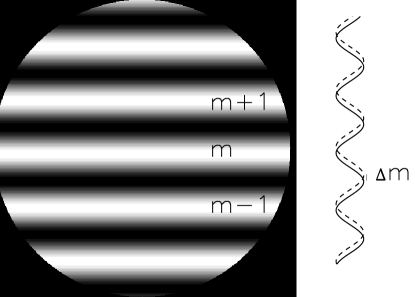
Figure 1.— This pattern shows the expected output when a field compensated Michelson interferometer with a small tilt in one arm is illuminated with monochromatic light. The cartoon on the right shows the phase shift of the interferometer fringes when the wavelength of the light experiences a Doppler shift.

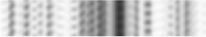
Figure 2.— Simulated two dimensional spectral format for a dispersed fixed-delay interferometer instrument. Fringes are clearly visible at the location of the stellar absorption lines.

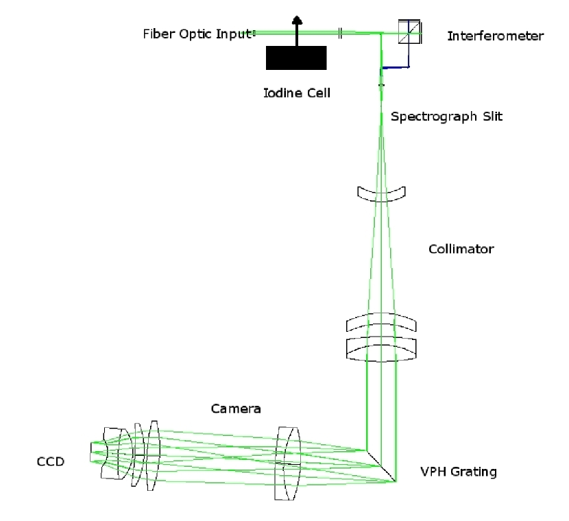
Figure 3.— Optical layout of the Kitt Peak ET instrument, showing the Michelson interferometer, spectrograph camera and collimator, VPH grating, and the iodine cell that can be inserted into the path of the collimated beam.

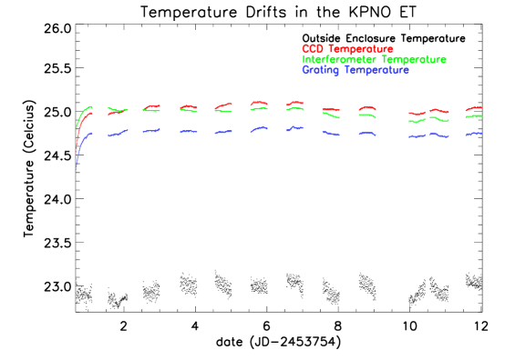
Figure 4.— The temperature measured at four points in the ET instrument during a typical observing run. The instrument enclosure helps stabilize the temperature and dampens the effect of the temperature variations outside the enclosure. The iodine cell and the electronics inside the detector head are the dominant source of heat inside the enclosure.

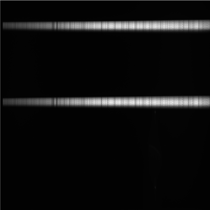
Figure 5.— The 4k $\times$ 4k pixles image obtained with ET instrument. Both outputs from the interferometer are imaged onto the detector. The two-dimensional spectral format allows the measurement of the fringe phase at each wavelength without having to physically change the interferometer delay.

Figure 6.— Optimal delay for a K5V star at different rotational velocities. The optimal value of the interferometer delay maximizes $\gamma d$. This maximum value of $\gamma d$ has been normalized to one for all the plots.

Figure 7.— Phase shift for a compensated Michelson interferometer that has $L_{1}$(BK7) $=4.04$ mm, $L_{2}$(air) $=2.66$ mm. The wavelength dependent phase shift show here is for a converging beam with a half angle of 1.5 degrees.

Figure 8.— Exploded view of the monolithic Michelson interferometer showing each component of the final assembly.

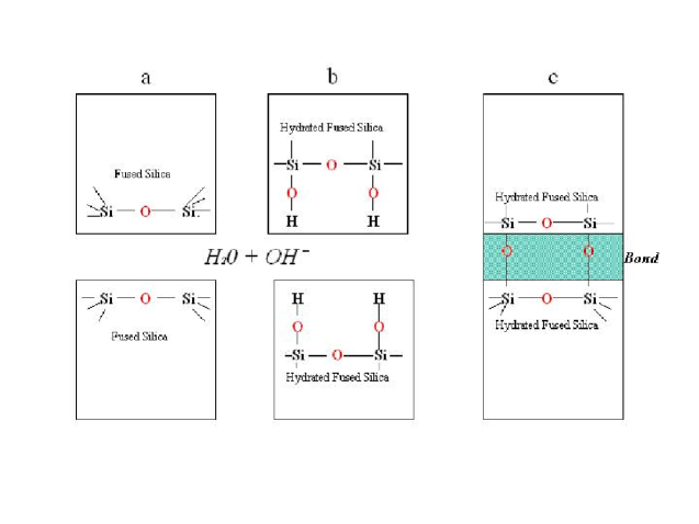
Figure 9.— The formation of a bond between two fused silica disks in the presence of water and the hydroxide catalyst. A similar mechanism occurs for any material capable of forming a silicate-like network. In this figure a) shows the fused silica disks, b) demonstrates the formation of hydrated fused silica, and c) shows the formations of a bond linking the two disks. This figure is adapted from Gwo (2003).

Figure 10.— The velocity drift of a passive interferometer during lab testing. The interferometer was placed in a vacuum chamber and the fringes were monitored using a stabilized He-Ne laser and a LabView program.

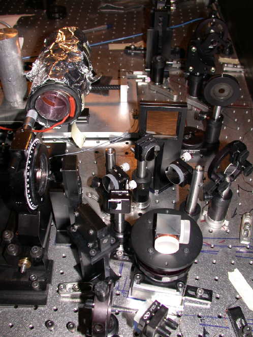
Figure 11.— The assembled monolithic interferometer aligned in the Kitt Peak ET instrument. The copper spacer and the BK7 arm of the interferometer are clearly visible. Also seen are the iodine cell, the input optics and the slit assembly.

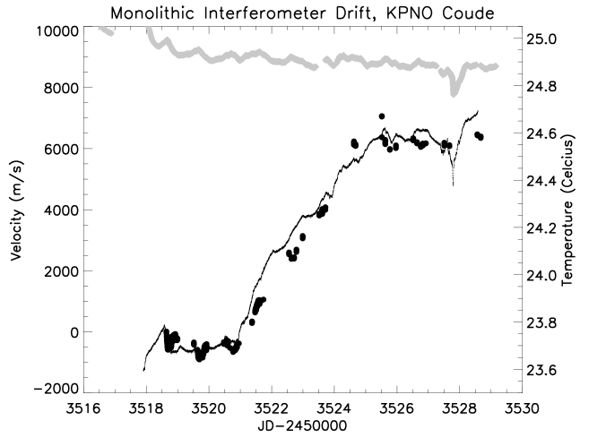
Figure 12.— The velocity drift of the monolithic interferometer during an observing run at Kitt Peak, as measured with a stabilized He-Ne laser, is shown as solid black line. Filled circles are the measured drift of the iodine calibration spectra obtained during the run. The grey line shows the measured interferometer temperature.

Figure 13.— Radial velocity obtained with the monolithic interferometer. The stars selected are the known radial velocity stable stars $\eta$ Cas and 36 UMa , and the known planet bearing stars 55 Cnc and $\rho$ Crb. The expected velocity amplitude caused by the known planetary systems is plotted as a solid line.

References

- Barden (1998) Barden, S. C. 1998, in ASP Conf. Ser. 152: Fiber Optics in Astronomy III, ed. S. Arribas, E. Mediavilla, & F. Watson, 14
- Beckers& Brown (1979) Beckers, J. M., & Brown, T. M. 1979, Oss. Mem. Oss. Astrofis. Arcetri, Fasc. 106, p. 189 - 203, 106, 189
- Borucki et al. (2003) Borucki, W. J., et al. 2003, Proc. SPIE, 4854, 129
- Bouchy et al. (2001) Bouchy, F., Pepe, F., & Queloz, D. 2001, A&A, 374, 733
- Butler et al. (1996) Butler, R. P., Marcy, G. W., Williams, E., McCarthy, C., Dosanjh, P., & Vogt, S. S. 1996, PASP, 108, 500
- Butler et al. (2006) Butler, R. P., Wright, J. T., Marcy, G. W., Fischer, D. A., Vogt, S. S., Tinney, C. G., Jones, H. R. A., Carter, B. D., Johnson, J. A., McCarthy, C., & Penny, A. J. 2006, ApJ, 646, 505
- Connes et al. (1996) Connes, P., Martic, M., & Schmitt, J. 1996, Ap&SS, 241, 61
- Endl et al. (2007) Endl, M., Cochran, W. D., Wittenmyer, R. A., & Boss, A. P. 2007, ArXiv e-prints, 709, arXiv:0709.0944
- Englert et al. (2007) Englert, C. R., Stevens, M. H., Siskind, D. E., Harlander, J. M., & Roesler, F. L. 2007, AGU Fall Meeting Abstracts, 1
- Erskine (2003) Erskine, D. J. 2003, PASP, 115, 255
- Erskine & Ge (2000) Erskine, D. J., & Ge, J. 2000, in ASP Conf. Ser. 195: Imaging the Universe in Three Dimensions, ed. W. van Breugel & J. Bland-Hawthorn, 501
- Forrest & Ring (1978) Forrest, A. K., & Ring, J. 1978, High resolution spectrometry, 462
- Gault et al. (1985) Gault, W. A., Johnston, S. F., & Kendall, D. J. W. 1985, Appl. Opt., 24, 1604
- Ge (2002) Ge, J. 2002, ApJ, 571, L165
- Ge et al. (2002) Ge, J., Erskine, D. J., & Rushford, M. 2002, PASP, 114, 1016
- Ge et al. (2003) Ge, J., van Eyken, J. C., Mahadevan, S., DeWitt, C., Ramsey, L. W., Shaklan, S. B., & Pan, X. 2003, Proc. SPIE, 4838, 503
- Ge et al. (2004) Ge, J., Mahadevan, S., van Eyken, J. C., DeWitt, C., Friedman, J., & Ren, D. 2004, Proc. SPIE, 5492, 711
- Ge et al. (2006) Ge, J., et al. 2006, ApJ,648, 683
- Ge et al. (2007) Ge, J., et al. 2007, American Astronomical Society Meeting Abstracts, 211, #132.09
- Gwo (1998) Gwo, D.-H. 1998, Proc. SPIE, 3435, 136
- Gwo (1998) Gwo, D.-H. 1998, Proc. SPIE, 3356, 892
- Gwo (2001) Gwo, D. 2001, United States Patent 6284085
- Gwo (2003) Gwo, D. 2003, United States Patent 6284085
- Harvey & The GONG Instrument Team (1995) Harvey, J., & The GONG Instrument Team. 1995, in ASP Conf. Ser. 76: GONG 1994. Helio- and Astro-Seismology from the Earth and Space, ed. R. K. Ulrich, E. J. Rhodes, Jr., & W. Dappen, 432
- Heacox (1986) Heacox, W. D. 1986, AJ, 92, 219
- Hilliard & Shepherd (1966) Hilliard, R. L., & Shepherd, G. G. 1966, Journal of the Optical Society of America (1917-1983), 56, 362
- Hunter & Ramsey (1992) Hunter, T. R., & Ramsey, L. W. 1992, PASP, 104, 1244
- Johnson et al. (2007) Johnson, J. A., et al. 2007, ApJ, 665, 785
- Kogelnik (1969) Kogelnik, H. 1969, The Bell System Technical Journal, Vol. 48, no. 9, November 1969, pp. 2909-2947, 48, 2909
- Kozhevatov (1983) Kozhevatov, I. E. 1983, Issledovaniia Geomagnetizmu Aeronomii i Fizike Solntsa, 64, 42
- Mahadevan et al. (2008) Mahadevan, S., van Eyken, J., Ge, J., DeWitt, C., Fleming, S. W., Cohen, R., Crepp, J., & Vanden Heuvel, A. 2008, ApJ, 678, 1505
- Mayor & Queloz (1995) Mayor, M., & Queloz, D. 1995, Nature, 378, 355
- McMillan et al. (1994) McMillan, R. S., Moore, T. L., Perry, M. L., & Smith, P. H. 1994, Ap&SS, 212, 271
- Mosser et al. (1998) Mosser, B., Maillard, J. P., Mekarnia, D., & Gay, J. 1998, A&A, 340, 457
- Mosser et al. (2003) Mosser, B., Maillard, J.-P., & Bouchy, F. 2003, PASP, 115, 990
- Mosser & The Siamois Team (2007) Mosser, B., & The Siamois Team 2007, EAS Publications Series, 25, 239
- Ramsey & Huenemoerder (1986) Ramsey, L. W., & Huenemoerder, D. P. 1986, Proc. SPIE, 627, 282
- Rallison et al. (2003) Rallison, R. D., Rallison, R. W., & Dickson, L. D. 2003, in Specialized Optical Developments in Astronomy. Edited by Atad-Ettedgui, Eli; D’Odorico, Sandro. Proceedings of the SPIE, Volume 4842, pp. 10-21 (2003)., ed. E. Atad-Ettedgui & S. D’Odorico, 10
- Rivera et al. (2005) Rivera, E. J., Lissauer, J. J., Butler, R. P., Marcy, G. W., Vogt, S. S., Fischer, D. A., Brown, T. M., Laughlin, G., & Henry, G. W. 2005, ApJ, 634, 625
- Rupprecht et al. (2004) Rupprecht, G., Pepe, F., Mayor, M., Queloz, D., Bouchy, F., Avila, G., Benz, W., Bertaux, J.-L., Bonfils, X., Dall, T., Delabre, B., Dekker, H., Eckert, W., Fleury, M., Gilliotte, A., Gojak, D., Guzman, J. C., Kohler, D., Lizon, J.-L., Lo Curto, G., Longinotti, A., Lovis, C., Megevand, D., Pasquini, L., Reyes, J., Sivan, J.-P., Sosnowska, D., Soto, R., Udry, S., Van Kesteren, A., Weber, L., & Weilenmann, U. 2004, in Ground-based Instrumentation for Astronomy. Edited by Alan F. M. Moorwood and Iye Masanori. Proceedings of the SPIE, Volume 5492, pp. 148-159 (2004)., ed. A. F. M. Moorwood & M. Iye, 148
- Santos et al. (2004) Santos, N. C., Bouchy, F., Mayor, M., Pepe, F., Queloz, D., Udry, S., Lovis, C., Bazot, M., Benz, W., Bertaux, J.-L., Lo Curto, G., Delfosse, X., Mordasini, C., Naef, D., Sivan, J.-P., & Vauclair, S. 2004, A&A, 426, L19
- Setiawan et al. (2007) Setiawan, J., Weise, P., Henning, T., Launhardt, R., Müller, A., & Rodmann, J. 2007, ApJ, 660, L145
- Shao et al. (2007) Shao, M., et al. 2007, ArXiv e-prints, 704, arXiv:0704.0952
- Shepherd et al. (1985) Shepherd, G. G., Gault, W. A., Miller, D. W., Pasturczyk, Z., Johnston, S. F., Kosteniuk, P. R., Haslett, J. W., Kendall, D. J. W., & Wimperis, J. R. 1985, Appl. Opt., 24, 1571
- Thuillier & Shepherd (1985) Thuillier, G., & Shepherd, G. G. 1985, Appl. Opt., 24, 1599
- Title & Ramsey (1980) Title, A. M., & Ramsey, H. E. 1980, Appl. Opt., 19, 2046
- van Eyken et al. (2003) van Eyken, J. C., Ge, J. C., Mahadevan, S., DeWitt, C., & Ren, D. 2003, Proc. SPIE, 5170, 250
- van Eyken et al. (2004) van Eyken, J. C., Ge, J., Mahadevan, S., & DeWitt, C. 2004, ApJ, 600, L79
- Wolszczan & Frail (1992) Wolszczan, A., & Frail, D. A. 1992, Nature, 355, 145