Linearized model Fokker–Planck collision operators for gyrokinetic simulations.
II. Numerical implementation and tests

Abstract

A set of key properties for an ideal dissipation scheme in gyrokinetic simulations is proposed, and implementation of a model collision operator satisfying these properties is described. This operator is based on the exact linearized test-particle collision operator, with approximations to the field-particle terms that preserve conservation laws and an H-Theorem. It includes energy diffusion, pitch-angle scattering, and finite Larmor effects corresponding to classical (real-space) diffusion. The numerical implementation in the continuum gyrokinetic code GS2 is fully implicit and guarantees exact satisfaction of conservation properties. Numerical results are presented showing that the correct physics is captured over the entire range of collisionalities, from the collisionless to the strongly collisional regimes, without recourse to artificial dissipation.

I Introduction

Collisions play an important role in gyrokinetics. An accurate collision operator is important for calculation of neoclassical transport Bolton and Ware (1983); Xu (2008) and the growth rate of instabilities such as trapped electron modes, Ernst et al. (2004, 2006) dissipative drift waves, Federici et al. (1987); Rewoldt and Tang (1990); Kotschenreuther et al. (1995) and microtearing modes Applegate et al. (2007) in moderate collisionality regimes. Collisions can also affect the damping of zonal flows Xiao et al. (2007) and other modes that provide a sink for turbulent energy. In their absence, arbitrarily fine scales can develop in phase space, Krommes and Hu (1994); Krommes (1999); Schekochihin et al. (2007, 2008); Barnes and Dorland (2008) which can in some cases pose challenges for discrete numerical algorithms, especially in the long-time limit; Grant and Feix (1967); Nevins et al. (2005) even a modest amount of collisions can make accurate numerical calculation much easier.

Furthermore, inclusion of a small collisionality keeps the distribution function smooth enough in velocity space that the standard gyrokinetic ordering Frieman and Chen (1982) for velocity space gradients is satisfied. For example, the parallel nonlinearity, Villard et al. (2004); Candy et al. (2006) given by

$$-\frac{\partial}{\partial v_{\parallel}}\left[h\left(\frac{q}{m}\mathbf{\hat{b}}+v_{\parallel}\frac{\mathbf{\hat{b}}\times\nabla B}{B^{2}}\right)\cdot\nabla\left<\varphi\right>\right]$$ (1)

enters at the same order as the other terms in the gyrokinetic equation if the typical scale of parallel velocity fluctuations, $\delta v_{\parallel}$, is one order smaller in the gyrokinetic expansion parameter $\rho/L$ ($\rho\equiv\textnormal{gyroradius}$ and $L\equiv\textnormal{background scale length}$) than the thermal speed, $v_{th}$. Here, $h$ is the non-Boltzmann part of the perturbed distribution function (defined more rigorously in the next section), $\varphi$ is the electrostatic potential, $B$ is the magnetic field strength, $\mathbf{\hat{b}}\equiv\mathbf{B}/B$, $q$ is particle charge, $m$ is particle mass, and $\left<\ .\ \right>$ denotes the gyroaverage at fixed guiding center position $\mathbf{R}$.

While such a situation is possible in the collisionless limit, a small collisionality prohibits the formation of structures with $\delta v_{\parallel}\sim(\rho/L)v_{th}$. The level of collisionality necessary to negate the importance of the parallel nonlinearity can be calculated by assuming a balance between collisions and fluctation dynamics:

$$\frac{\partial h}{\partial t}\sim C[h]\Rightarrow\omega h\sim\nu v_{th}^{2}\frac{\partial^{2}h}{\partial v^{2}},$$ (2)

where $C[h]$ describes the effect of collisions on $h$, $\omega$ is the fluctuation frequency, and $\nu$ is the collision frequency. From the above expression, we see that scales in velocity space become small enough for the parallel nonlinearity to be important only when the collision frequency satisfies $\nu\sim(\rho/L)^{2}\omega$. Such low collisionalities are not present in most fusion plasmas of interest. Furthermore, if such an ordering had to be adopted, the lowest order distribution function could become strongly non-Maxwellian. This is a problem for $\delta f$ codes that assume an equilibrium Maxwellian.

In light of the above considerations, it is important to include an accurate treatment of dissipation in gyrokinetic simulations. In order to faithfully represent gyrokinetic plasma dynamics at reasonable numerical expense, we take the view that the form of the dissipation should be such that it: ensures satisfaction of the standard gyrokinetic ordering; locally conserves particle number, momentum, and energy; satisfies Boltzmann’s $H$-Theorem; and efficiently smooths phase space structure. The first of these requirements has already been discussed in the context of the parallel nonlinearity. Conservation properties have been found to be important, for instance, in calculations of the neoclassical ion thermal conductivity, Hinton and Hazeltine (1976) as well as in a wide range of problems in fluid dynamics. The existence of an $H$-Theorem is critical for entropy balance Krommes and Hu (1994); Sugama et al. (1996); Howes et al. (2006) and for the dynamics of the turbulent phase space cascade. Schekochihin et al. (2007, 2008) Efficient smoothing of phase space structures is necessary to resolve numerical simulations at reasonable computational expense.

A commonly employed dissipation mechanism in gyrokinetic simulations is artificial (hyper) dissipation, often in physical (position) space. Kotschenreuther et al. (1995); Jenko et al. (2000); Candy and Waltz (2006); Barnes and Dorland (2008); Chen and Parker (2007) Ideally, the form of the artificial dissipation should be chosen to satisfy the requirements listed above and should be tested for convergence to the collisionless result. Of course, artificial dissipation alone is unable to capture the correct dynamics for moderate to strongly collisional systems where turbulent fluxes and other observable quantities depend sensitively on collisionality; for such systems, a physical dissipation model is desired.

A number of such model physical collision operators are employed in gyrokinetic codes. Kotschenreuther et al. (1995); Jenko et al. (2000); Candy and Waltz (2006); Navkal et al. (2006) These range in complexity from the Krook operator Rewoldt et al. (1986) to the Rutherford-Kovrizhnikh operator Rutherford et al. (1970) to the Catto-Tsang operator, Catto and Tsang (1976) all of which have previously been implemented in GS2 (see, e.g. Ref. Navkal et al., 2006). However, none of these satisfy all of the properties we require of a good collision operator (See Appendix C of the accompanying paper Abel et al. (2008) for a fuller discussion of this point). Here, we discuss numerical implementation in GS2 of an improved model operator which: includes the effects of both pitch-angle scattering and energy diffusion (i.e. efficiently smooths in phase space and ensures gyrokinetic ordering); conserves particle number, momentum, and energy; satisfies Boltzmann’s $H$-Theorem; and reduces to the linearized Landau test-particle operator in the large $k_{\perp}\rho$ limit. A full description of this operator and a discussion of its desirable properties, including comparison with the previous models of Catto-Tsang and Hirshman-Sigmar, Hirshman and Sigmar (1976) is given in the companion paper Abel et al. (2008) (henceforth Paper I). We will focus on how such an operator can be implemented efficiently in gyrokinetic codes while maintaining the properties listed above and on how our gyrokinetic dissipation scheme (or any other) might be tested against a number of plasma physics problems.

The paper is organized as follows: in Section II, we introduce the gyroaveraged collision operator from Paper I and examine properties that should be taken into account when using it in numerical simulations; in Section III, we describe our numerical implementation of the collision operator; in Section IV we present numerical results for a number of tests demonstrating the ability of our collision operator implementation to reproduce correct collisional and collisionless physics; and in Section V, we summarize our findings.

II Properties of the gyroaveraged collision operator

In order to include collisions in gyrokinetics, we follow the treatment of Ref. Howes et al., 2006 and assume the collision frequency, $\nu$, to be the same order in the gyrokinetic ordering as the characteristic fluctuation frequency, $\omega$. This leads to the requirement that the distribution of particles in velocity space is Maxwellian to lowest order and allows us to represent the total distribution function through first order in $\rho/L$ (where $\rho$ is ion gyroradius and $L$ is the scale length of equilibrium quantities) as

$$f(\mathbf{r},\mu,\varepsilon,t)=F_{0}(\varepsilon)\left(1-\frac{q\varphi(\mathbf{r},t)}{T_{0}}\right)+h(\mathbf{R},\mu,\varepsilon,t),$$ (3)

where $\mathbf{r}$ is particle position, $\mathbf{R}=\mathbf{r}-\mathbf{\hat{b}}\times\mathbf{v}/\Omega_{0}$ is guiding center position, $\mu\equiv mv_{\perp}^{2}/2B_{0}$ is magnetic moment, $\varepsilon\equiv mv^{2}/2$ is particle energy, $F_{0}$ is a Maxwellian, $\varphi$ is the electrostatic potential, $B_{0}$ is the magnitude of the background magnetic field, $T_{0}$ is the background temperature, $q$ is particle charge, and $\Omega_{0}=qB_{0}/mc$. The gyrokinetic equation governing the evolution of $h$ is given by

$$\begin{split}\frac{\partial h}{\partial t}&+\left(v_{\parallel}\mathbf{\hat{b}}+\mathbf{v}_{D}\right)\cdot\frac{\partial h}{\partial\mathbf{R}}+\frac{c}{B_{0}}\{\left<\chi\right>_{\mathbf{R}},h\}\\ &=-q\frac{\partial F_{0}}{\partial\varepsilon}\frac{\partial\left<\chi\right>_{\mathbf{R}}}{\partial t}+\frac{c}{B_{0}}\{F_{0},\left<\chi\right>_{\mathbf{R}}\}+\left<C[h]\right>_{\mathbf{R}},\end{split}$$ (4)

where $\mathbf{\hat{b}}\equiv\mathbf{B}_{0}/B_{0}$, $\mathbf{v}_{D}$ is the drift velocity of guiding centers, $\chi\equiv\varphi-\mathbf{v}\cdot\mathbf{A}/c$, $\mathbf{A}$ is the vector potential, $\{a,b\}$ is the Poisson bracket of $a$ and $b$, $\left<a\right>_{\mathbf{R}}$ is the gyroaverage of $a$ at constant $\mathbf{R}$, and $\left<C[h]\right>_{\mathbf{R}}$ is the gyroaveraged collision operator.

For $\left<C[h]\right>_{\mathbf{R}}$, we restrict our attention to the model collision operator presented in Paper I. We work within the framework of the continuum gyrokinetic code GS2, Kotschenreuther et al. (1995) which assumes periodicity in the spatial directions perpendicular to $\mathbf{B}_{0}$ in order to reduce the simulation volume to a thin flux tube encompassing a single magnetic field line. Consequently, we require a spectral representation of $\left<C[h]\right>_{\mathbf{R}}$:

$$\left<C[h]\right>_{\mathbf{R}}\equiv\sum_{\mathbf{k}}e^{i\mathbf{k}\cdot\mathbf{R}}C_{GK}[h_{\mathbf{k}}],$$ (5)

where $\mathbf{k}$ is the perpendicular wavevector. For convenience, we reproduce the expression for the same-species part of $C_{GK}[h_{\mathbf{k}}]$ from Paper I in operator form:

$$C_{GK}[h_{\mathbf{k}}]\equiv L[h_{\mathbf{k}}]+D[h_{\mathbf{k}}]+U_{L}[h_{\mathbf{k}}]+U_{D}[h_{\mathbf{k}}]+E[h_{\mathbf{k}}],$$ (6)

where

$$L[h_{\mathbf{k}}]\equiv\frac{\nu_{D}}{2}\frac{\partial}{\partial\xi}\left(1-\xi^{2}\right)\frac{\partial h_{\mathbf{k}}}{\partial\xi}-\frac{k^{2}v^{2}}{4\Omega_{0}^{2}}\nu_{D}\left(1+\xi^{2}\right)h_{\mathbf{k}}$$ (7)

and

$$D[h_{\mathbf{k}}]\equiv\frac{1}{2v^{2}}\frac{\partial}{\partial v}\left(\nu_{\parallel}v^{4}F_{0}\frac{\partial}{\partial v}\frac{h_{\mathbf{k}}}{F_{0}}\right)-\frac{k^{2}v^{2}}{4\Omega_{0}^{2}}\nu_{\parallel}\left(1-\xi^{2}\right)h_{\mathbf{k}}$$ (8)

are the gyroaveraged Lorentz and energy diffusion operators (which together form the test-particle piece of the linearized Landau operator, as shown in Refs Catto and Tsang, 1976 and Abel et al., 2008),

$$\begin{split}U_{L}[h_{\mathbf{k}}]\equiv\nu_{D}F_{0}\Big{(}&J_{0}(\alpha)v_{\parallel}\frac{\int d^{3}v\ \nu_{D}v_{\parallel}J_{0}(\alpha)h_{\mathbf{k}}}{\int d^{3}v\ \nu_{D}v_{\parallel}^{2}F_{0}}\\ &+J_{1}(\alpha)v_{\perp}\frac{\int d^{3}v\ \nu_{D}v_{\perp}J_{1}(\alpha)h_{\mathbf{k}}}{\int d^{3}v\ \nu_{D}v_{\parallel}^{2}F_{0}}\Big{)}\end{split}$$ (9)

and

$$\begin{split}U_{D}[h_{\mathbf{k}}]\equiv-\Delta\nu&F_{0}\Big{(}J_{0}(\alpha)v_{\parallel}\frac{\int d^{3}v\ \Delta\nu v_{\parallel}J_{0}(\alpha)h_{\mathbf{k}}}{\int d^{3}v\ \Delta\nu v_{\parallel}^{2}F_{0}}\\ &+J_{1}(\alpha)v_{\perp}\frac{\int d^{3}v\ \Delta\nu v_{\perp}J_{1}(\alpha)h_{\mathbf{k}}}{\int d^{3}v\ \Delta\nu v_{\parallel}^{2}F_{0}}\Big{)}\end{split}$$ (10)

are the gyroaveraged momentum-conserving corrections to the Lorentz and energy diffusion operators, and

$$E[h_{\mathbf{k}}]\equiv\nu_{E}v^{2}J_{0}(\alpha)F_{0}\frac{\int d^{3}v\ \nu_{E}v^{2}J_{0}(\alpha)h_{\mathbf{k}}}{\int d^{3}v\ \nu_{E}v^{4}F_{0}}$$ (11)

is the gyroaveraged energy-conserving correction (the conserving terms are an approximation to the field-particle piece of the linearized Landau operator). The electron collision operator has the following additional term to account for electron-ion collisions:

$$\begin{split}C_{GK}^{ei}[h_{e,\mathbf{k}}]=\nu_{D}^{ei}\Big{(}\frac{1}{2}\frac{\partial}{\partial\xi}&\left(1-\xi^{2}\right)\frac{\partial h_{e,\mathbf{k}}}{\partial\xi}-\frac{k^{2}v^{2}}{4\Omega_{0_{e}}^{2}}\left(1+\xi^{2}\right)h_{e,\mathbf{k}}\\ &+\frac{2v_{\parallel}u_{\parallel}[h_{i,\mathbf{k}}]}{v_{th_{e}}^{2}}J_{0}(\alpha_{e})F_{0e}\Big{)},\end{split}$$ (12)

where $\xi\equiv v_{\parallel}/v$ is the pitch angle, $\alpha\equiv kv_{\perp}/\Omega_{0}$, $J_{0}$ and $J_{1}$ are Bessel functions of the first kind, $v_{th}\equiv\sqrt{2T_{0}/m}$ is the thermal velocity, and $u_{\parallel}[h_{i,\mathbf{k}}]$ is the perturbed parallel ion flow velocity. Expressions for the velocity-dependent collision frequencies $\nu_{D}$, $\Delta\nu$, $\nu_{\parallel}$, and $\nu_{E}$ are given in Paper I (which follows the notation of Ref. Hirshman and Sigmar, 1976).

Having specified the form of our collision operator, we now discuss some of its fundamental properties that guide our choice of numerical implementation.

II.1 Collision operator amplitude

Even when the collisionality approaches zero, $C_{GK}[h_{\mathbf{k}}]$ can have appreciable amplitude. There are two reasons for this: first, the velocity dependence of $\nu_{D}$, $\nu_{E}$, and $\Delta\nu$ is such that each go to infinity as $v\rightarrow 0$ (so low-velocity particles are always collisional); and second, we expect the distribution function to develop increasingly smaller scales in $v$ and $\xi$ as collisionality decreases, so that the amplitude of the terms proportional to $\partial^{2}h/\partial\xi^{2}$ and $\partial^{2}h/\partial v^{2}$ may remain approximately constant (i.e. $C_{GK}[h_{\mathbf{k}}]\not\rightarrow 0$ as $\nu\rightarrow 0$). Krommes and Hu (1994); Krommes (1999); Schekochihin et al. (2007); Barnes and Dorland (2008) The fact that $C_{GK}[h_{\mathbf{k}}]$ can be quite large even at very low collisionalities means that it should be treated implicitly if one wants to avoid a stability limit on the size of the time step, $\Delta t$. In Section III, we describe our fully implicit implementation of the collision operator.

II.2 Local moment conservation

Since collisions locally conserve particle density, momentum, and energy, one would like these properties to be guaranteed by the discrete version of the collision operator. Mathematically, this means that the density, momentum, and energy moments of the original (un-gyroaveraged) collision operator must vanish (for same-species collisions). However, the non-local nature of the gyroaveraging operation introduces finite Larmor radius (FLR) effects that lead to nonzero values for the analogous moments of $\left<C[h]\right>_{\mathbf{R}}$. Since this is the quantity we employ in gyrokinetics, we need to find the pertinent relations its moments must satisfy in order to guarantee local conservation properties.

This is accomplished by Taylor expanding the Bessel functions $J_{0}$ and $J_{1}$. In particular, one can show that Abel et al. (2008)

$$\begin{split}&\int d^{3}v\begin{pmatrix}1\\ \mathbf{v}\\ v^{2}\end{pmatrix}\left<\left<C[h]\right>_{\mathbf{R}}\right>_{\mathbf{r}}\\ &=\sum_{\mathbf{k}}e^{i\mathbf{k}\cdot\mathbf{r}}\int d^{3}v\begin{pmatrix}1\\ v_{\parallel}\mathbf{\hat{b}}\\ v^{2}\end{pmatrix}C_{GK}^{0}[h_{\mathbf{k}}]-\nabla\cdot\Gamma_{C},\end{split}$$ (13)

where $\left<.\right>_{\mathbf{r}}$ denotes a gyroaverage at fixed $\mathbf{r}$, $C_{GK}^{0}[h_{\mathbf{k}}]$ is the operator of Eqn. (6) with $k\rho=0$ (neglecting FLR terms but retaining nonzero subscripts $\mathbf{k}$ for $h$), and $\Gamma_{C}$ is the collisional flux of number, momentum, and energy arising from FLR terms. Consequently, the density, momentum, and energy moments of the gyrokinetic equation can be written in the conservative form

$$\frac{\partial\mathcal{M}}{\partial t}+\nabla\cdot\Gamma_{\mathcal{M}}=\int d^{3}v\begin{pmatrix}1\\ v_{\parallel}\mathbf{\hat{b}}\\ v^{2}\end{pmatrix}C_{GK}^{0}[h_{\mathbf{k}}],$$ (14)

where $\mathcal{M}\equiv\left(\delta n\ n\delta\mathbf{u}_{\parallel}\ \delta p\right)^{T}$ represents the perturbed number, momentum, and energy densities, the superscript $T$ denotes the transpose, and $\Gamma_{\mathcal{M}}$ contains both the collisional flux, $\Gamma_{C}$, and the flux arising from all other terms in the gyrokinetic equation (for a more detailed discussion, see Paper I). Thus, local conservation properties are assured in gyrokinetics as long as the density, momentum, and energy moments of $C_{GK}^{0}[h_{\mathbf{k}}]$ vanish:

$$\int d^{3}v\begin{pmatrix}1\\ v_{\parallel}\\ v^{2}\end{pmatrix}C_{GK}^{0}[h_{\mathbf{k}}]=0.$$ (15)

We describe how this is accomplished numerically in Section III.

II.3 $H$-Theorem

In contrast with local conservation properties, the statement of the $H$-Theorem is unmodified by gyroaveraging the collision operator. Defining the entropy as $S=-f\ln f$, Boltzmann’s $H$-Theorem tells us

$$\frac{\partial S}{\partial t}=-\int\frac{d^{3}\mathbf{r}}{V}\int d^{3}v\ \ln[f]C[f]\geq 0,$$ (16)

where $V\equiv\int d^{3}\mathbf{r}$ and the double integration spans phase space (the velocity integration is taken at constant particle position $\mathbf{r}$). Expanding the distribution function as before, we find to lowest order in the gyrokinetic ordering

$$\int\frac{d^{3}\mathbf{r}}{V}\int d^{3}v\ \frac{h}{F_{0}}C[h]\leq 0.$$ (17)

Changing variables from particle position $\mathbf{r}$ to guiding center position $\mathbf{R}$, we obtain

$$\int d^{3}v\int\frac{d^{3}\mathbf{R}}{V}\ \frac{h}{F_{0}}\left<C[h]\right>_{\mathbf{R}}\leq 0,$$ (18)

where now the velocity integration is taken at constant $\mathbf{R}$. In this case, the non-locality of the gyroaveraging operation leads to no modification of the $H$-Theorem because of the definition of entropy as a phase-space averaged quantity (as opposed to local conservation properties, which involve only velocity-space averages). Therefore, one can easily diagnose entropy generation and test numerical satisfaction of the $H$-Theorem in gyrokinetic simulations, as we show in Sec. IV.

III Numerical implementation

It is convenient for numerical purposes to separately treat collisional and collisionless physics. Thus, we begin by writing the gyrokinetic equation in the form

$$\frac{\partial h_{\mathbf{k}}}{\partial t}=C_{GK}[h_{\mathbf{k}}]+\mathcal{A}[h_{\mathbf{k}}],$$ (19)

where $\mathcal{A}[h_{\mathbf{k}}]$ represents the rate of change of $h_{\mathbf{k}}$ due to the collisionless physics. In order to separate these terms, we utilize Godunov dimensional splitting, Godunov (1959) which is accurate to first order in the timestep $\Delta t$:

$$\frac{h^{*}_{\mathbf{k}}-h^{n}_{\mathbf{k}}}{\Delta t}=\mathcal{A}[h^{n}_{\mathbf{k}},h^{*}_{\mathbf{k}}]$$ (20)

$$\frac{h^{n+1}_{\mathbf{k}}-h^{*}_{\mathbf{k}}}{\Delta t}=C_{GK}[h^{n+1}_{\mathbf{k}}],$$ (21)

where $n$ and $n+1$ are indices representing the current and future time steps, and $h^{*}_{\mathbf{k}}$ is defined by Eqn. (20) – it is the result of advancing the collisionless part of the gyrokinetic equation. With $h^{*}_{\mathbf{k}}$ thus given, we restrict our attention to solving Eqn. (21). For notational convenience, we suppress all further $\mathbf{k}$ subscripts, as we will be working exclusively in $k$-space.

As argued in Section II, we must treat the collision operator implicitly to avoid a stability limit on the size of $\Delta t$. We use a first order accurate backward-difference scheme in time instead of a second order scheme (such as Crank-Nicholson Richtmyer and Morton (1967)) because it is well known that the Crank-Nicholson scheme introduces spurious behavior in solutions to diffusion equations when taking large timesteps (and because Godunov splitting is only first order accurate for multiple splittings, which will be introduced shortly).

With this choice, $h^{n+1}$ is given by

$$h^{n+1}=\left(1-\Delta tC_{GK}\right)^{-1}h^{*}.$$ (22)

In general, $C_{GK}$ is a dense matrix, with both energy and pitch-angle indices. Inversion of such a matrix, which is necessary to solve for $h^{n+1}$ in our implicit scheme, is computationally expensive. We avoid this by taking two additional simplifying steps. First we employ another application of the Godunov splitting technique, which, combined with the choice of a $(\xi,v)$ grid in GS2, Barnes and Dorland (2008) allows us to consider energy and pitch-angle dependence separately: 

$$h^{**}=\left[1-\Delta t\left(L+U_{L}\right)\right]^{-1}h^{*}$$ (23)

$$h^{n+1}=\left[1-\Delta t\left(D+U_{D}+E\right)\right]^{-1}h^{**},$$ (24)

The $h^{*}$ and $h^{**}$ are vectors whose components are the values of $h$ at each of the $(\xi,v)$ grid points. In Eqn. (23) we order the components so that

$$h\equiv\left(h_{11},h_{21},...,h_{N1},h_{12},...,h_{NM}\right)^{T},$$ (25)

where the first index represents pitch-angle, the second represents energy, and $N$ and $M$ are the number of pitch-angle and energy grid points, respectively. This allows for a compact representation in pitch-angle. When solving Eqn. (24), we reorder the components of $h$ so that

$$h\equiv\left(h_{11},h_{12},...,h_{1N},h_{21},...,h_{NM}\right)^{T},$$ (26)

allowing for a compact representation in energy.

III.1 Conserving terms

The matrices $1-\Delta tL$ and $1-\Delta tD$ are chosen to be tridiagonal by employing three-point stencils for finite differencing in $\xi$ and $v$. This permits computationally inexpensive matrix inversion. However, the full matrices to be inverted include the momentum- and energy-conserving operators, $U$ and $E$, which are dense matrices. We avoid direct inversion of these matrices by employing the Sherman-Morrison formula, Sherman and Morrison (1949, 1950) which gives $\mathbf{x}$ in the matrix equation $M\mathbf{x}=\mathbf{b}$, as long as $M$ can be written in the following form:

$$M=A+\mathbf{u}\otimes\mathbf{v},$$ (27)

where $\otimes$ is the tensor product. The solution is then given by

$$\mathbf{x}=\mathbf{y}-\left[\frac{\mathbf{v}\cdot\mathbf{y}}{1+\mathbf{v}\cdot\mathbf{z}}\right]\mathbf{z},$$ (28)

where $\mathbf{y}=A^{-1}\mathbf{b}$, $\mathbf{z}=A^{-1}\mathbf{u}$, and the dot products represent integrals over velocity space. If $A^{-1}$ is known or easily obtainable (as in our case), this formulation provides significant computational savings over the straighforward method of directly inverting the dense matrix $M$.

Details of the application of the Sherman-Morrison formula to Eqns. (23) and (24) are given in Appendix A. Here, we state the main points. The matrix operators $L$ and $D$ are to be identified with $A$, and the integral conserving terms $U$ and $E$ can be written in the form of the tensor product, $\mathbf{u}\otimes\mathbf{v}$. Identifying $h^{**}$ and $h^{n+1}$ with $\mathbf{x}$, we find that multiple applications of the Sherman-Morrison formula give

$$h=\mathbf{y}_{2}-\left[\frac{\mathbf{v}_{2}\cdot\mathbf{y}_{2}}{1+\mathbf{v}_{2}\cdot\mathbf{z}_{2}}\right]\mathbf{z}_{2},$$ (29)

where

$$\mathbf{y}_{2}=\mathbf{y}_{0}-\left[\frac{\mathbf{v}_{0}\cdot\mathbf{y}_{0}}{1+\mathbf{v}_{0}\cdot\mathbf{s}_{0}}\right]\mathbf{s}_{0}-\left[\frac{\mathbf{v}_{1}\cdot\mathbf{y}_{0}}{1+\mathbf{v}_{1}\cdot\mathbf{w}_{0}}\right]\mathbf{w}_{0},$$ (30)

$$\mathbf{z}_{2}=\mathbf{z}_{0}-\left[\frac{\mathbf{v}_{0}\cdot\mathbf{z}_{0}}{1+\mathbf{v}_{0}\cdot\mathbf{s}_{0}}\right]\mathbf{s}_{0}-\left[\frac{\mathbf{v}_{1}\cdot\mathbf{z}_{0}}{1+\mathbf{v}_{1}\cdot\mathbf{w}_{0}}\right]\mathbf{w}_{0}.$$ (31)

The quantities $\mathbf{v}_{0}$, $\mathbf{v}_{1}$, $\mathbf{v}_{2}$, $\mathbf{z}_{0}$, $\mathbf{s}_{0}$, $\mathbf{w}_{0}$, and $\mathbf{y}_{0}$ are specified in Table 1 in Appendix A. With the exception of $\mathbf{y}_{0}$, each of these quantities is time-independent, so they need be computed only once at the beginning of each simulation. Consequently, inclusion of the conserving terms in our implicit scheme comes at little additional expense.

We note that when Eqn. (29) is applied to computing the inverse matrix in Eqn. (23), the corresponding $\mathbf{v}_{2}$ is nonzero only for the electron collision operator. This term arises by using the parallel component of Ampere’s law to rewrite the electron-ion collison operator of Eqn. (12) as

$$\begin{split}C_{GK}^{ei}[h_{e}]&=\nu_{D}^{ei}\Bigg{(}\frac{1}{2}\frac{\partial}{\partial\xi}\left(1-\xi^{2}\right)\frac{\partial h_{e}}{\partial\xi}-\frac{k^{2}v^{2}}{4\Omega_{0,e}^{2}}\left(1+\xi^{2}\right)h_{e}\\ &+\frac{2v_{\parallel}}{v_{th_{e}}^{2}}J_{0}(\alpha_{e})F_{0e}\left[u_{\parallel}[h_{e}]+\frac{ck^{2}}{4\pi en_{0,e}}A_{\parallel}\right]\Bigg{)},\end{split}$$ (32)

where $e$ is the magnitude of the electron charge, $u_{\parallel}[h_{e}]$ is the parallel component of the electron fluid velocity, and $n_{0,e}$ is the equilibrium electron density. For electron collisions, the $A_{\parallel}$ term is absorbed into $h^{*}$ so that we use the modified quantity

$$\tilde{h}_{e}^{*}=h_{e}^{*}+\nu_{D}^{ei}\Delta t\frac{ck^{2}v_{\parallel}}{2\pi ev_{th_{e}}^{2}n_{0,e}}A_{\parallel}J_{0}(\alpha_{e})F_{0,e}$$ (33)

when applying the Sherman-Morrison formula, where $A_{\parallel}$ from the $n+1$ time level is used (for details on the implicit calculation of $A_{\parallel}$, see Ref. Kotschenreuther et al., 1995).

III.2 Discretization in energy and pitch angle

We still must specify our choice of discretization for $C_{GK}$. Ideally, we would like the discrete scheme to guarantee the conservation properties and $H$-Theorem associated with $C$. As discussed in Sec. II, the former is equivalent to requiring that the $k\rho=0$ component of $C_{GK}$, $C_{GK}^{0}$, satisfy Eqn. (15). We now proceed to show that this requirement is satisfied by carefully discretizing the conserving terms and by employing a novel finite difference scheme that incorporates the weights associated with our numerical integration scheme.

We begin by writing $C_{GK}^{0}[h]$ for same-species collisions:

$$\begin{split}C_{GK}^{0}[h]&=\frac{\nu_{D}}{2}\frac{\partial}{\partial\xi}\left(1-\xi^{2}\right)\frac{\partial h}{\partial\xi}+\frac{1}{2v^{2}}\frac{\partial}{\partial v}\left(\nu_{\parallel}v^{4}F_{0}\frac{\partial}{\partial v}\frac{h}{F_{0}}\right)+\nu_{D}v_{\parallel}F_{0}\frac{\int d^{3}v\ \nu_{D}v_{\parallel}h}{\int d^{3}v\ \nu_{D}v_{\parallel}^{2}F_{0}}\\ &-\Delta\nu v_{\parallel}F_{0}\frac{\int d^{3}v\ \Delta\nu v_{\parallel}h}{\int d^{3}v\ \Delta\nu v_{\parallel}^{2}F_{0}}+\nu_{E}v^{2}F_{0}\frac{\int d^{3}v\ \nu_{E}v^{2}h}{\int d^{3}v\ \nu_{E}v^{4}F_{0}}.\end{split}$$ (34)

With $C_{GK}^{0}$ thus specified, we now consider numerical evaluation of the relevant moments of Eqn. (34). To satisfy number conservation ($\int d^{3}v\ C_{GK}^{0}[h]=0$), velocity space integrals of each of the terms in Eqn. (34) should vanish individually. For integrals of the first two terms to vanish, we require a finite difference scheme that satisfies a discrete analog of the Fundamental Theorem of Calculus (i.e. conservative differencing); for the last three terms, we must have a discrete integration scheme satisfying $\int d^{3}v\ \nu_{D}v_{\parallel}F_{0}=\int d^{3}v\ \Delta\nu v_{\parallel}F_{0}=\int d^{3}v\ \nu_{E}v^{2}F_{0}=0$. The requirement that $\int d^{3}v\ \nu_{D}v_{\parallel}F_{0}=\int d^{3}v\ \Delta\nu v_{\parallel}F_{0}=0$ is satisfied by any integration scheme with velocity space grid points and associated integration weights symmetric about $v_{\parallel}=0$, which is true for the $(\xi,v)$ grid used in GS2. By substituting for $\nu_{E}$ everywhere using the identity

$$\nu_{E}v^{2}F_{0}=-\frac{1}{v^{2}}\frac{\partial}{\partial v}\left(\nu_{\parallel}v^{5}F_{0}\right),$$ (35)

the other integral constraint ($\int d^{3}v\ \nu_{E}v^{2}F_{0}=0$) reduces to the requirement that finite difference schemes must satisfy the Fundamental Theorem of Calculus.

Parallel momentum conservation ($\int d^{3}v\ v_{\parallel}C_{GK}^{0}[h]=0$) introduces the additional requirements that:

$$\int d^{3}v\ v_{\parallel}\left(\frac{\nu_{D}}{2}\frac{\partial}{\partial\xi}\left(1-\xi^{2}\right)\frac{\partial h}{\partial\xi}+v_{\parallel}\nu_{D}F_{0}\frac{\int d^{3}v\ \nu_{D}v_{\parallel}h}{\int d^{3}v\ \nu_{D}v_{\parallel}^{2}F_{0}}\right)=0$$ (36)

and

$$\begin{split}\int d^{3}v\ &\frac{v_{\parallel}}{2v^{2}}\frac{\partial}{\partial v}\left(\nu_{\parallel}v^{4}F_{0}\frac{\partial}{\partial v}\frac{h}{F_{0}}\right)\\ &=\int d^{3}v\ \Delta\nu v_{\parallel}^{2}F_{0}\frac{\int d^{3}v\ \Delta\nu v_{\parallel}h}{\int d^{3}v\ \Delta\nu v_{\parallel}^{2}F_{0}}.\end{split}$$ (37)

If the finite difference scheme used for all differentiation possesses a discrete version of integration by parts (upon double application), then Eqns. (36) and $(\ref{eqn:vpaD})$ are numerically satisfied as long as: $v_{\parallel}\nu_{D}h$ in the second term of Eqn. (36) is expressed in the form

$$v_{\parallel}\nu_{D}h=-\frac{1}{2}\left(\frac{\partial}{\partial\xi}\left(1-\xi^{2}\right)\frac{\partial v_{\parallel}}{\partial\xi}\right)\nu_{D}h,$$ (38)

$\Delta\nu$ on the righthand side of Eqn. (37) is expressed using the identity

$$2\Delta\nu v^{3}F_{0}=\frac{\partial}{\partial v}\left(\nu_{\parallel}v^{4}F_{0}\frac{\partial v}{\partial v}\right),$$ (39)

and all integrals are computed using the same numerical integration scheme (if analytic results for the integral denominators in terms 3 and 4 of Eqn. (34) are used, then the necessary exact cancellation in Eqns. (36) and (37) will not occur).

The only additional constraint imposed by energy conservation ($\int d^{3}v\ v^{2}C_{GK}^{0}[h]=0$) is that the form of Eqn. (35) be slightly modified so that

$$\nu_{E}v^{2}F_{0}=-\frac{1}{v^{2}}\frac{\partial}{\partial v}\left(\nu_{\parallel}v^{4}F_{0}\frac{\partial v^{2}}{\partial v}\right),$$ (40)

which still satisfies the number conservation contraint. Using the forms given by Eqns. (38)-(40), conservation properties are guaranteed as long as one employs a finite difference scheme for pitch-angle scattering and energy diffusion that satisfies discrete versions of the Fundamental Theorem of Calculus and integration by parts.

For the case of equally spaced grid points in $v$ and $\xi$, there is a straightforward difference scheme, accurate to secord order in the grid spacing, that satisfies both requirements: Degond and Lucquin-Desreux (1994)

$$\frac{\partial}{\partial x}G\frac{\partial h}{\partial x}\approx\frac{G_{j+1/2}\left(h_{j+1}-h_{j}\right)-G_{j-1/2}\left(h_{j}-h_{j-1}\right)}{\Delta x^{2}},$$ (41)

where $x$ is a dummy variable representing either $v$ or $\xi$, $\Delta x$ is the grid spacing, $h_{j}$ is the value of $h$ evaluated at the grid point $x_{j}$, $x_{j\pm 1/2}\equiv(x_{j}+x_{j\pm 1})/2$, and $G$ is either $1-\xi^{2}$ (for pitch-angle scattering) or $\nu_{\parallel}v^{4}F_{0}$ (for energy diffusion). However, in order to achieve higer order accuracy in the calculation of the velocity space integrals necessary to obtain electromagnetic fields, GS2 Barnes and Dorland (2008) and a number of other gyrokinetic codes Candy and Waltz (2003) use grids with unequal spacing in $v$ and $\xi$ and integration weights that are not equal to the grid spacings.

Given the constraints of a three-point stencil on an unequally spaced grid, we are forced to choose between a higher order scheme (a second order accurate scheme can be obtained with compact differencing, Durran (1999) as described in Appendix B) that does not satisfy our two requirements and a lower order scheme that does. Since our analytic expression for $C_{GK}$ was designed in large part to satisfy conservation properties (and because the conserving terms are only a zeroth order accurate approximation to the field-particle piece of the linearized Landau operator Hirshman and Sigmar (1976)), we choose the lower order scheme, given here, as the default:

$$\frac{\partial}{\partial x}G\frac{\partial h}{\partial x}\approx\frac{1}{w_{j}}\left(G_{j+1/2}\frac{h_{j+1}-h_{j}}{x_{j+1}-x_{j}}-G_{j-1/2}\frac{h_{j}-h_{j-1}}{x_{j}-x_{j-1}}\right),$$ (42)

where $w_{j}$ is the integration weight associated with $x_{j}$.

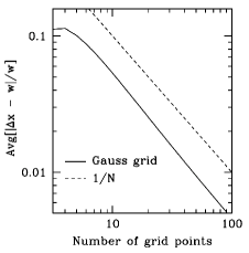
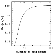
Figure 1: (Left): Solid line indicates the scaling of the leading order error, averaged over all grid points, of the conservative finite difference scheme for a Gauss-Legendre grid (the grid used in GS2). The slope of the dotted line corresponds to a first order scheme. (Right): factor by which the conservative finite difference scheme of Eqn. (42) amplifies the true collision operator amplitude at the boundaries of the Gauss-Legendre grid.

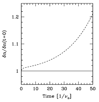
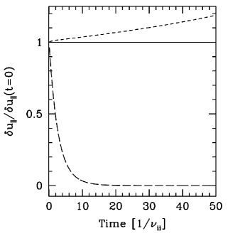
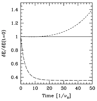
Figure 2: Plots showing evolution of the perturbed local density, parallel momentum, and energy over fifty collision times. Without the conserving terms (9)-(11), both parallel momentum and energy decay significantly over a few collision times (long dashed lines). Inclusion of conserving terms with the conservative scheme detailed in Sec. III leads to exact moment conservation (solid lines). Use of a non-conservative scheme leads to inexact conservation that depends on grid spacing (short dashed lines).

Defining $\Psi\equiv Gh^{\prime}$, with the prime denoting differentiation with respect to $x$, Taylor series can be used to show

$$\frac{\Psi_{j+1/2}-\Psi_{j-1/2}}{w_{j}}=\Psi^{\prime}_{j}\frac{\Delta x_{j}}{w_{j}}+\mathcal{O}\left(\frac{\left(\Delta x\right)_{j}^{2}}{w_{j}}\right),$$ (43)

where $\Delta x_{j}=x_{j+1/2}-x_{j-1/2}$. With the exception of pitch angles corresponding to trapped particles, Barnes and Dorland (2008); Kotschenreuther et al. (1995) the grid points $\{x_{j}\}$ and associated integration weights $\{w_{j}\}$ in GS2 are chosen according to Gauss-Legendre quadrature rules. Hildebrand (1987) For this case, we show numerically in Fig. 1 that

$$\frac{1}{N}\sum_{j=1}^{N}\frac{\Delta x_{j}}{w_{j}}=1+\mathcal{O}\left(\frac{1}{N}\sum_{j=1}^{N}\Delta x_{j}\right)=1+\mathcal{O}\left(\frac{1}{N}\right),$$ (44)

and

$$\max_{j=2,...,N-1}\left|1-\frac{\Delta x_{j}}{w_{j}}\right|=\mathcal{O}\left(\frac{1}{N}\right),$$ (45)

where $N$ is the number of grid points in $x$.

The boundary points ($j=1,N$) are excluded from the $\max$ operator above. This is because $\Delta x/w$ (the factor multiplying $\Psi_{j}^{\prime}$ in Eqn. (43)) converges to approximately 1.2 for the boundary points as the grid spacing is decreased (Fig. 1). For the energy diffusion operator, we can make use of the property that $G(x)=G(x)^{\prime}=0$ at $x=0$ and $x=\infty$ to show

$$\pm\frac{\Psi_{j\pm 1/2}}{w_{j}}=\Psi_{j}^{\prime}+\mathcal{O}\left(\frac{\left(\Delta x\right)_{j}^{2}}{w_{j}}\right),$$ (46)

with the plus sign corresponding to $j=1$ and the minus sign to $j=N$. This is not true for the Lorentz operator, so we are forced to accept an approximately twenty percent magnification of the Lorentz operator amplitude at $\xi=\pm 1$ and at the trapped-passing boundaries. We find that this relatively small error at the boundaries has a negligible effect on measureable (velocity space averaged) quantities in our simulations.

IV Numerical tests

We now proceed to demonstrate the validity of our collision operator implementation. In particular, we demonstrate conservation properties, satisfaction of Boltzmann’s $H$-Theorem, efficient smoothing in velocity space, and recovery of theoretically expected results in both collisional (fluid) and collisionless limits. While we do not claim that the suite of tests we have performed is exhaustive, it constitutes a convenient set of numerical benchmarks that can be used for validating collision operators in gyrokinetics.

IV.1 Homogeneous plasma slab

We first consider the long wavelength limit of a homogeneous plasma slab with Boltzmann electrons and no variation along the magnetic field ($k_{\parallel}=0$). The gyrokinetic equation for this system simplifies to

$$\frac{\partial\left(\delta f\right)}{\partial t}\approx C_{GK}^{0}[h],$$ (47)

which means local density, momentum, and energy should be conserved. In Fig. 2 we show numerical results for the time evolution of the local density, momentum, and energy for this system.

Without inclusion of the conserving terms (9)-(11), we see that density is conserved, as guaranteed by the conservative differencing scheme, while the momentum and energy decay away over several collision times. Inclusion of the conserving terms provides us with exact (up to numerical precision) conservation of number, momentum, and energy. To illustrate the utility of our conservative implementation, we also present results from a numerical scheme that does not make use of Eqns. (38)-(40) and that employs a finite difference scheme that does not possess discrete versions of the Fundamental Theorem of Calculus and integration by parts. Specifically, we consider a first order accurate finite difference scheme similar to that given by Eqn. (42), with the only difference being that the weights in the denominator are replaced with the local grid spacings. In this case, we see that density, momentum, and energy are not exactly conserved (how well they are conserved depends on velocity space resolution, which is 16 pitch angles and 16 energies for the run considered here).

The rate at which our collision operator generates entropy in the homogenous plasma slab is shown in Fig. 3. As required by the $H$-Theorem, the rate of entropy production is always nonnegative and approaches zero in the long-time limit as the distribution function approaches a shifted Maxwellian. We find this to hold independent of both the grid spacing in velocity space and the initial condition for the distribution function (in Fig. 3, the values of $h(\xi,v)$ were drawn randomly from the uniform distribution on the interval $[-1/2,1/2]$).

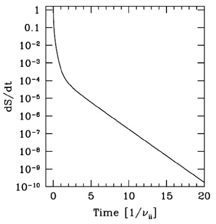
Figure 3: Plot of the evolution of entropy generation for the homogeneous plasma slab over twenty collision times. Our initial distribution in velocity space is random noise, and we use a grid with 16 pitch angles and 8 energies. The entropy generation rate is always nonnegative and approaches zero in the long-time limit.

IV.2 Resistive damping

We now modify the system above by adding a finite $A_{\parallel}$. From fluid theory, we know that collisional friction between electrons and ions provides resistivity which leads to the decay of current profiles. Because the resistive time is long compared to the collision time, one can neglect $\partial(\delta f)/\partial t$. However, since $A_{\parallel}\sim k^{-2}$, and we are considering $k\ll 1$, $\partial A_{\parallel}/\partial t$ must be retained. The resulting electron equation is of the form of the classical Spitzer problem (see, e.g., Ref. Helander and Sigmar, 2002):

$$C_{GK}^{0}[h_{e}]=-\frac{eF_{0,e}}{T_{0,e}}\frac{v_{\parallel}}{c}\frac{\partial A_{\parallel}}{\partial t}.$$ (48)

The parallel current evolution for this system is given by

$$J_{\parallel}(t)=J_{\parallel}(t=0)e^{-\eta t},$$ (49)

where $\eta=1/\sigma_{\parallel}$ is the resistivity, $\sigma_{\parallel}=1.98\tau_{e}n_{e}e^{2}/m_{e}c^{2}$ is the Spitzer conductivity, and $\tau_{e}=3\sqrt{\pi}/4\nu_{ei}$ is the electron collision time.

We demonstrate that the numerical implementation of our operator correctly captures this resistive damping in Figs. 4 and 5. We also see in these figures that in the absence of the ion drag term from Eqn. (12), the electron flow is incorrectly damped to zero (instead of to the ion flow), leading to a steady-state current.

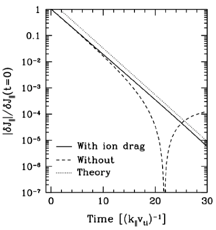
Figure 4: Evolution of $|J_{\parallel}|$ for the electromagnetic plasma slab with $\beta=10^{-4}$, $k_{y}\rho_{i}=0.1$, and $\nu_{ei}=10k_{\parallel}v_{th,i}$. Inclusion of the ion drag term in the electron-ion collision operator leads to the theoretically predicted damping rate for the parallel current given in Eqn. (49) . Without the ion drag term, the parallel current decays past zero (at $t\approx 22$) and converges to a negative value as the electron flow damps to zero.

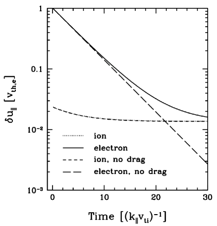
Figure 5: Evolution of perturbed parallel flow for the electromagnetic plasma slab with $\beta=10^{-4}$, $k_{y}\rho_{i}=0.1$, and $\nu_{ei}=10k_{\parallel}v_{ti}$. Without inclusion of the ion drag term in Eqn. (12), the electron flow is erroneously damped to zero (instead of to the ion flow).

IV.3 Slow mode damping

We next consider the damping of the slow mode in a homogenous plasma slab as a function of collisionality. In the low $k_{\perp}\rho_{i}$, high $\beta_{i}$ limit, one can obtain analytic expressions for the damping rate in both the collisional ($k_{\parallel}\lambda_{mfp}\ll 1$) and collisionless ($k_{\parallel}\lambda_{mfp}\gg 1$) regimes, where $\lambda_{mfp}$ is the ion mean free path (see e.g. Ref. Schekochihin et al., 2007). The expressions are

$$\omega=\pm k_{\parallel}v_{A}\sqrt{1-\left(\frac{\nu_{\parallel,i}k_{\parallel}}{2v_{A}}\right)^{2}}-i\frac{\nu_{\parallel,i}k_{\parallel}^{2}}{2}$$ (50)

for $k_{\parallel}\lambda_{mfp}\ll 1$, and

$$\omega=-i\frac{\left|k_{\parallel}\right|v_{A}}{\sqrt{\pi\beta_{i}}}$$ (51)

for $k_{\parallel}\lambda_{mfp}\gg 1$. Here, $v_{A}=v_{th,i}/\sqrt{\beta_{i}}$ is the Alfven speed, and $\nu_{\parallel,i}$ is the parallel ion viscosity, which is inversely proportial to the ion-ion collision frequency, $\nu_{ii}$: $\nu_{\parallel,i}\propto v_{th,i}^{2}/\nu_{ii}$. As one would expect, the damping in the strongly collisional regime [Eqn. (50)] is due primarily to viscosity, while the collisionless regime [Eqn. (51)] is dominated by Barnes damping. Barnes (1966)

In Fig. 6, we plot the collisional dependence of the damping rate of the slow mode obtained numerically using the new collision operator implementation in GS2. In order to isolate the slow mode in these simulations, we took $\varphi=A_{\parallel}=\delta n_{e}=0$ and measured the damping rate of $\delta B_{\parallel}$. This is possible because $\delta B_{\parallel}$ effectively decouples from $\varphi$ and $A_{\parallel}$ for our system, and $\delta n_{e}$ can be neglected because $\beta_{i}\gg 1$. Schekochihin et al. (2007) We find quantitative agreement with the analytic expressions (50) and (51) in the appropriate regimes. In particular, we recover the correct viscous behavior in the $k_{\parallel}\lambda_{mfp}\ll 1$ limit (damping rate proportional to $\nu_{\parallel,i}$), the correct collisional damping in the $k_{\parallel}\lambda_{mfp}\sim 1$ limit (damping rate inversely proportial to $\nu_{\parallel,i}$), and the correct collisionless (i.e. Barnes) damping in the $k_{\parallel}\lambda_{mfp}\gg 1$ limit.

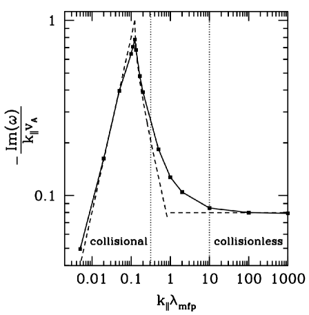
Figure 6: Damping rate of the slow mode for a range of collisionalities spanning the collisionless to strongly collisional regimes. Dashed lines correspond to the theoretical prediction for the damping rate in the collisional ($k_{\parallel}\lambda_{mfp}\ll 1$) and collisionless ($k_{\parallel}\lambda_{mfp}\gg 1$) limits. The solid line is the result obtained numerically with GS2. Vertical dotted lines denote approximate regions (collisional and collisionless) for which the analytic theory is valid.

IV.4 Electrostatic turbulence

Finally, we illustrate the utility of our collision operator in a nonlinear simulation of electrostatic turbulence in a Z-pinch field configuration. Freidberg (1987) We consider the Z-pinch because it contains much of the physics of toroidal configurations (i.e. curvature) without some of the complexity (no particle trapping). At relatively weak pressure gradients, the dominant gyrokinetic linear instability in the Z-pinch is the entropy mode, Kadomtsev (1960); Kesner (2000); Simakov et al. (2001, 2002); Kesner and Hastie (2002); Ricci et al. (2006a) which is nonlinearly unstable to secondary instabilities such as Kelvin-Helmholtz. Ricci et al. (2006b)

In previous numerical investigations of linear Ricci et al. (2006a) and nonlinear Ricci et al. (2006b) plasma dynamics in a Z-pinch, collisions were found to play an important role in the damping of zonal flows and in providing an effective energy cutoff at short wavelengths. However, as pointed out in Ref. Ricci et al., 2006b, the Lorentz collision operator used in those investigations provided insufficient damping of short wavelength structures to obtain steady-state fluxes. Consequently, a model hyper-viscosity had to be employed.

We have reproduced a simulation from Ref. Ricci et al., 2006b using our new collison operator, and we find that hyper-viscosity is no longer necessary to obtain steady-state fluxes (Fig. 7). This can be understood by examining the linear growth rate spectrum of Fig. 8. We see that in this system energy diffusion is much more efficient at suppressing short wavelength structures than pitch-angle scattering. Consequently, no artificial dissipation of short wavelength structures is necessary.

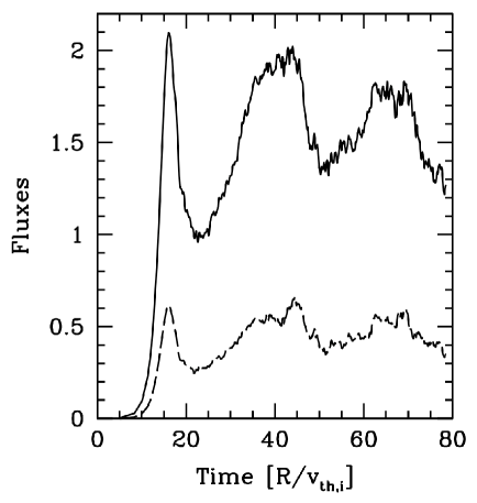
Figure 7: Evolution of ion particle and heat fluxes for an electrostatic, 2-species Z-pinch simulation. We are considering $R/L_{n}=2.0$ and $\nu_{ii}=0.01v_{th,i}/R$. The particle flux is indicated by the solid line and is given in units of $(\rho/R)n_{0,i}v_{th,i}$. The heat flux is indicated by the dashed line and is given in units of $(\rho/R)n_{0,i}v_{th,i}^{2}$. We see that a steady-state is achieved for both fluxes without artificial dissipation.

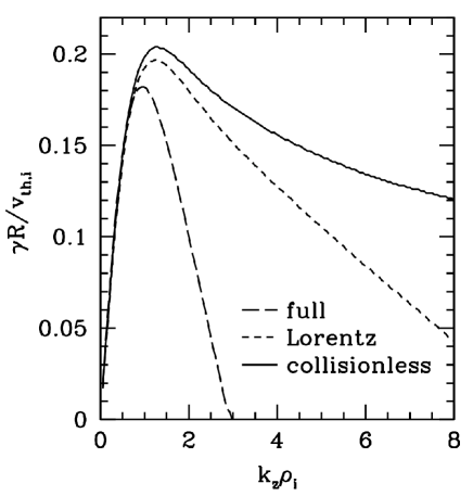
Figure 8: Linear growth rate spectrum of the entropy mode in a Z-pinch for $R/L_{n}=2.0$, where $R$ is major radius and $L_{n}$ is density gradient scale length. The solid line is the collisionless result, and the two dashed lines represent the result of including collisions. The short dashed line corresponds to using only the Lorentz operator, while the long dashed line corresponds to using our full model collision operator. Both collisional cases were carried out with $\nu_{ii}=0.01v_{th,i}/R$.

V Summary

In Sec. I we proposed a set of key properties that an ideal dissipation scheme for gyrokinetics should satisfy. Namely, the scheme should: limit the scale size of structures in phase space in order to guarantee the validity of the gyrokinetic ordering and to provide numerical resolution at reasonable expense; conserve particle number, momentum, and energy; and satisfy Boltzmann’s $H$-Theorem. While commonly employed simplified collision operators or hyperviscosity operators may be adequate for some calculations, Dimits et al. (2000) it is important to be able to use the more complete collision operator described in this paper, which preserves all of these desirable dissipation properties.

In Sec. II we presented the model collision operator derived in Paper I and discussed some of its features that strongly influence our choice of numerical implementation. In particular, we noted that local conservation properties are guaranteed as long as the ($1$, $v_{\parallel}$, $v^{2}$) moments of the $k\rho=0$ component of the gyroaveraged collision operator vanish. Further, we argued that the collision operator should be treated implicitly because in some regions of phase space, its amplitude can be large even at very small collisionalities.

Our numerical implementation of the collision operator was described in Sec. III. We separate collisional and collisionless physics through the use of Godunov dimensional splitting and advance the collision operator in time using a backwards Euler scheme. The test particle part of the collision operator is differenced using a scheme that possesses discrete versions of the Fundamental Theorem of Calculus and integration by parts (upon double application). These properties are necessary in order to exactly satisfy the desired conservation properties in the long wavelength limit. The field particle response is treated implicitly with little additional computational expense by employing repeated application of the Sherman-Morrison formula, as detailed in Appendix A.

In Sec. IV we presented numerical tests to demonstrate that our implemented collision operator possesses the properties required for a good gyrokinetic dissipation scheme. In addition to these basic properties, we showed that the implemented collision operator allows us to correctly capture physics phenomena ranging from the collisionless to the strongly collisional regimes. In particular, we provided examples for which we are able to obtain quantitatively correct results for collisionless (Landau or Barnes), resistive, and viscous damping.

In conclusion, we note that resolution of the collisionless (and collisional) physics in our simulations was obtained solely with physical collisions; no recourse to any form of artificial numerical dissipation was necessary.

VI Appendix A: Sherman-Morrison Formulation

The repeated application of the Sherman-Morrison formula considered here is an extension of the scheme presented in Tatsuno and Dorland. Tatsuno and Dorland (2008) Throughout this calculation, we adopt general notation applicable to both Eqns. (23) and (24) and provide specific variable definitions in Table 1. Both Eqns. (23) and (24) can be written in the form

$$A\mathbf{x}=\mathbf{b}.$$ (52)

variable	$L$	$D$
$A$	$\ 1-\Delta t\left(L+U_{L}\right)\$	$\ 1-\Delta t\left(D+U_{D}+E\right)\$
$\mathbf{x}$	$h^{**}$	$h^{n+1}$
$\mathbf{b}$	$h^{*}$	$h^{**}$
$A_{0}$	$1-\Delta tL$	$1-\Delta tD$
$\mathbf{v}_{0}$	$\nu_{D}v_{\perp}J_{1}$	$-\Delta\nu v_{\perp}J_{1}$
$\mathbf{v}_{1}$	$\nu_{D}v_{\parallel}J_{0}$	$-\Delta\nu v_{\parallel}J_{0}$
$\mathbf{v}_{2}$	$v_{\parallel}$ (electrons)	$\nu_{E}v^{2}J_{0}$
	$0$ (ions)
$\mathbf{u}_{0}$	$-\Delta t\mathbf{v}_{0}/d_{u}$	$-\Delta t\mathbf{v}_{0}/d_{u}$
$\mathbf{u}_{1}$	$-\Delta t\mathbf{v}_{1}/d_{u}$	$-\Delta t\mathbf{v}_{1}/d_{u}$
$\mathbf{u}_{2}$	$-\Delta t\nu_{D}^{ei}v_{\parallel}/d_{q}$ (electrons)	$-\Delta t\mathbf{v}_{2}/d_{q}$
	$0$ (ions)
$d_{u}$	$\int d^{3}v\ \nu_{D}v_{\parallel}^{2}F_{0}$	$\int d^{3}v\ \Delta\nu v_{\parallel}^{2}F_{0}$
$d_{q}$	$v_{th,e}^{2}/2$	$\int d^{3}v\ \nu_{E}v^{4}F_{0}$

Table 1: Sherman-Morrison variable definitions for Lorentz and energy diffusion operator equations

Because $\left<\mathcal{U}\right>$ and $\left<\mathcal{E}\right>$ are integral operators, we can write them as tensor products so that

$$A\equiv A_{0}+\mathbf{u}_{0}\otimes\mathbf{v}_{0}+\mathbf{u}_{1}\otimes\mathbf{v}_{1}+\mathbf{u}_{2}\otimes\mathbf{v}_{2}.$$ (53)

We now define

$$A_{1}=A_{0}+\mathbf{u}_{0}\otimes\mathbf{v}_{0},\ \ A_{2}=A_{1}+\mathbf{u}_{1}\otimes\mathbf{v}_{1},$$ (54)

so that

$$\left(A_{2}+\mathbf{u}_{2}\otimes\mathbf{v}_{2}\right)\mathbf{x}=\mathbf{b}.$$ (55)

Applying the Sherman-Morrison formula to this equation, we find

$$\mathbf{x}=\mathbf{y}_{2}-\frac{\mathbf{v}_{2}\cdot\mathbf{y}_{2}}{1+\mathbf{v}_{2}\cdot\mathbf{z}_{2}}\mathbf{z}_{2},$$ (56)

where $A_{2}\mathbf{y}_{2}=\mathbf{b}$ and $A_{2}\mathbf{z}_{2}=\mathbf{u}_{2}$.

Applying the Sherman-Morrison formula to each of these equations gives

$$\mathbf{y}_{2}=\mathbf{y}_{1}-\frac{\mathbf{v}_{1}\cdot\mathbf{y}_{1}}{1+\mathbf{v}_{1}\cdot\mathbf{w}_{1}}\mathbf{w}_{1}$$ (57)

$$\mathbf{z}_{2}=\mathbf{z}_{1}-\frac{\mathbf{v}_{1}\cdot\mathbf{z}_{1}}{1+\mathbf{v}_{1}\cdot\mathbf{w}_{1}}\mathbf{w}_{1},$$ (58)

where $A_{1}\mathbf{y}_{1}=\mathbf{b}$, $A_{1}\mathbf{w}_{1}=\mathbf{u}_{1}$, and $A_{1}\mathbf{z}_{1}=\mathbf{u}_{2}$. A final application of Sherman-Morrison to these three equations yields

$$\mathbf{y}_{1}=\mathbf{y}_{0}-\frac{\mathbf{v}_{0}\cdot\mathbf{y}_{0}}{1+\mathbf{v}_{0}\cdot\mathbf{s}_{0}}\mathbf{s}_{0}$$ (59)

$$\mathbf{w}_{1}=\mathbf{w}_{0}-\frac{\mathbf{v}_{0}\cdot\mathbf{w}_{0}}{1+\mathbf{v}_{0}\cdot\mathbf{s}_{0}}\mathbf{s}_{0}$$ (60)

$$\mathbf{z}_{1}=\mathbf{z}_{0}-\frac{\mathbf{v}_{0}\cdot\mathbf{z}_{0}}{1+\mathbf{v}_{0}\cdot\mathbf{s}_{0}}\mathbf{s}_{0},$$ (61)

where $A_{0}\mathbf{y}_{0}=\mathbf{b}$, $A_{0}\mathbf{s}_{0}=\mathbf{u}_{0}$, $A_{0}\mathbf{w}_{0}=\mathbf{u}_{1}$, and $A_{0}\mathbf{z}_{0}=\mathbf{u}_{2}$.

We can simplify our expressions by noting that $\mathbf{v}_{0,1,2}$ and $\mathbf{u}_{0,1,2}$ have definite parity in $v_{\parallel}$. A number of inner products then vanish by symmetry, leaving the general expressions

$$\mathbf{y}_{2}=\mathbf{y}_{0}-\left[\frac{\mathbf{v}_{0}\cdot\mathbf{y}_{0}}{1+\mathbf{v}_{0}\cdot\mathbf{s}_{0}}\right]\mathbf{s}_{0}-\left[\frac{\mathbf{v}_{1}\cdot\mathbf{y}_{0}}{1+\mathbf{v}_{1}\cdot\mathbf{w}_{0}}\right]\mathbf{w}_{0}$$ (62)

$$\mathbf{z}_{2}=\mathbf{z}_{0}-\left[\frac{\mathbf{v}_{0}\cdot\mathbf{z}_{0}}{1+\mathbf{v}_{0}\cdot\mathbf{s}_{0}}\right]\mathbf{s}_{0}-\left[\frac{\mathbf{v}_{1}\cdot\mathbf{z}_{0}}{1+\mathbf{v}_{1}\cdot\mathbf{w}_{0}}\right]\mathbf{w}_{0}.$$ (63)

VII Appendix B: Compact differencing of the test-particle operator

In this appendix, we derive a second order accurate compact difference scheme for pitch-angle scattering and energy diffusion on an unequally spaced grid. The higher order of accuracy of this scheme is desirable, but it does not possess discrete versions of the Fundamental Theorem of Calculus and integration by parts when used with Gauss-Legendre quadrature (or any other integration scheme with grid spacings unequal to integration weights). Consequently, one should utilize this scheme only if integration weights and grid spacings are equal, or if exact satisfaction of conservation properties is not considered important.

For convenience, we begin by noting that Eqns. (23) and (24) can both be written in the general form

$$\left(\frac{\partial h}{\partial t}\right)_{C}=H\left(Gh^{\prime}\right)^{\prime}+S=H\left(G^{\prime}h^{\prime}+Gh^{\prime\prime}\right)+S,$$ (64)

where: for the Lorentz operator equation (23) we identify $H=1$, $G=\nu_{D}\left(1-\xi^{2}\right)/2$, $S=U_{L}[h]-k^{2}v^{2}\nu_{D}\left(1+\xi^{2}\right)h/4\Omega_{0}^{2}$, and the prime denotes differentiation with respect to $\xi$; and for the energy diffusion operator equation (24), we identify $H=1/2v^{2}F_{0}$, $G=\nu_{\parallel}v^{4}F_{0}$, $S=U_{D}[h]+E[h]-k^{2}v^{2}\nu_{\parallel}\left(1-\xi^{2}\right)h/4\Omega_{0}^{2}$, and the prime denotes differentiation with respect to $v$. Here, the $h$ we are using is actually normalized by $F_{0}$.

Employing Taylor Series expansions of $h$, we obtain the expressions

$$h_{i}^{\prime}=\frac{\delta_{-}^{2}\left(h_{i+1}-h_{i}\right)+\delta_{+}^{2}\left(h_{i}-h_{i-1}\right)}{\delta_{+}\delta_{-}\left(\delta_{+}+\delta_{-}\right)}+\mathcal{O}[\delta^{2}],$$ (65)

and

$$h_{i}^{\prime\prime}=2\frac{\delta_{-}\left(h_{i+1}-h_{i}\right)-\delta_{+}\left(h_{i}-h_{i-1}\right)}{\delta_{+}\delta_{-}\left(\delta_{+}+\delta_{-}\right)}+\frac{\delta_{-}-\delta_{+}}{3}h_{i}^{\prime\prime\prime}+\mathcal{O}[\delta^{2}],$$ (66)

where $i$ denotes evaluation at the velocity space gridpoint $x_{i}$, and $\delta_{\pm}\equiv\left|x_{i\pm 1}-x_{i}\right|$ (here $x$ is a dummy variable representing either $\xi$ or $v$). In order for the $h_{i}^{\prime\prime}$ expression to be second order accurate, we must obtain a first order accurate expression for $h_{i}^{\prime\prime\prime}$ in terms of $h_{i}$, $h_{i}^{\prime}$, and $h_{i}^{\prime\prime}$. We accomplish this by differentiating Eqn. (64) with respect to $x$:

$$\left(\frac{\partial h^{\prime}}{\partial t}\right)_{C}=H^{\prime}\left(Gh^{\prime}\right)^{\prime}+H\left(Gh^{\prime}\right)^{\prime\prime}+S^{\prime}$$ (67)

and rearranging terms to find

$$\begin{split}h_{i}^{\prime\prime\prime}&=\frac{1}{H_{i}G_{i}}\Big{[}\left(\frac{\partial h_{i}}{\partial t}\right)_{C}-H_{i}^{\prime}\left(G_{i}^{\prime}h_{i}^{\prime}+G_{i}h_{i}^{\prime\prime}\right)\\ &-H_{i}\left(G_{i}^{\prime\prime}h_{i}+2G_{i}^{\prime}h_{i}^{\prime\prime}\right)-S_{i}^{\prime}\Big{]}+\mathcal{O}[\delta],\end{split}$$ (68)

where, unless denoted otherwise, all quantities are taken at the $n+1$ time level. Plugging this result into Eqn. 66 and grouping terms, we have

$$\begin{split}\mu_{i}h_{i}^{\prime\prime}&=\frac{\delta_{-}-\delta_{+}}{3H_{i}G_{i}}\left[h_{i}^{\prime}\left(\frac{1}{\Delta t}-H_{i}^{\prime}G_{i}^{\prime}-H_{i}G_{i}^{\prime\prime}\right)-\frac{\left(h_{i}^{n}\right)^{\prime}}{\Delta t}-S_{i}^{\prime}\right]\\ &+2\frac{\delta_{-}\left(h_{i+1}-h_{i}\right)-\delta_{+}\left(h_{i}-h_{i-1}\right)}{\delta_{+}\delta_{-}\left(\delta_{+}+\delta_{-}\right)}+\mathcal{O}[\delta^{2}],\end{split}$$ (69)

where $\mu_{i}=1+\left(\delta_{+}-\delta_{-}\right)\left(H_{i}^{\prime}G_{i}+2H_{i}G_{i}^{\prime}\right)/3H_{i}G_{i}$, and we have taken $(\partial h/\partial t)_{C}=(h^{n+1}-h^{n})/\Delta t$. Using Eqn. (67) and the above result in Eqn. (64), we find

$$\begin{split}\left(\frac{\partial h}{\partial t}\right)_{C}&=h_{i}^{\prime}\left(H_{i}G_{i}^{\prime}-\frac{\delta_{+}+\delta_{-}}{3\mu_{i}}\left[\frac{1}{\Delta t}-H_{i}^{\prime}G_{i}^{\prime}-H_{i}G_{i}^{\prime\prime}\right]\right)\\ &+\frac{H_{i}G_{i}}{\mu_{i}}\left(2\frac{\delta_{-}\left(h_{i+1}-h_{i}\right)-\delta_{+}\left(h_{i}-h_{i-1}\right)}{\delta_{+}\delta_{-}\left(\delta_{+}+\delta_{-}\right)}\right.\\ &+\left.\frac{\delta_{+}+\delta_{-}}{3H_{i}G_{i}}\left[\frac{\left(h_{i}^{n}\right)^{\prime}}{\Delta t}+S_{i}^{\prime}\right]\right)+S_{i}+\mathcal{O}[\delta^{2}].\end{split}$$ (70)

This is the general compact differenced form to be used when solving Eqns. (23) and (24).

In order to illustrate how compact differencing affects the implicit solution using Sherman-Morrison, we present the result of using the particular form of $S$ for energy diffusion in Eqn. (70):

$$\begin{split}\frac{h_{i}^{n+1}-h_{i}^{n}}{\Delta t}&=\frac{h_{i+1}}{\delta_{+}\left(\delta_{+}+\delta_{-}\right)}\left(\frac{2H_{i}G_{i}}{\mu_{i}}+\delta_{-}\zeta_{i}\right)\\ &\frac{h_{i-1}}{\delta_{-}\left(\delta_{+}+\delta_{-}\right)}\left(\frac{2H_{i}G_{i}}{\mu_{i}}-\delta_{+}\zeta_{i}\right)\\ &\frac{h_{i}}{\delta_{-}\delta_{+}}\left(-\frac{2H_{i}G_{i}}{\mu_{i}}+\left(\delta_{+}-\delta_{-}\right)\zeta_{i}-\delta_{+}\delta_{-}K\tilde{\nu}_{s}\right)\\ &\frac{\sigma_{i}}{\Delta t}\Bigg{(}h_{i+1}^{n}\frac{\delta_{-}}{\delta_{+}\left(\delta_{+}+\delta_{-}\right)}-h_{i-1}^{n}\frac{\delta_{+}}{\delta_{-}\left(\delta_{+}+\delta_{-}\right)}\\ &+h_{i}^{n}\frac{\delta_{+}-\delta_{-}}{\delta_{+}\delta_{-}}\Bigg{)}+\tilde{U}_{\parallel}V_{\parallel}+\tilde{U}_{\perp}V_{\perp}+\tilde{U}_{q}q+\mathcal{O}[\delta^{2}],\end{split}$$ (71)

where

$$\sigma_{i}=\left(\delta_{+}-\delta_{-}\right)/3\mu_{i}$$

$$K=k^{2}v_{th}^{2}\left(1-\xi^{2}\right)/8\Omega_{0}^{2}$$

$$\zeta_{i}=H_{i}G_{i}^{\prime}-\sigma_{i}\left(1/\Delta t-H_{i}^{\prime}G_{i}^{\prime}-H_{i}G_{i}^{\prime\prime}+K\nu_{s}\right)$$

$$\nu_{s}=\nu_{\parallel}v_{th}^{2}/2v^{2}$$

$$\tilde{A}=A+\sigma A^{\prime}$$

$$U_{\perp,\parallel,q}=\mathbf{u}_{0,1,2}$$

$$V_{\perp,\parallel,q}=\mathbf{v}_{0,1,2}$$

with $\mathbf{u}$ and $\mathbf{v}$ given in Table 1.

We see that the only significant effects of compact differencing on numerical implementation are: modification of $h^{**}$ in Eqn. (24) to reflect the $h^{n}$ terms on the right-hand side of Eqn. (71); and modification of the $U_{\parallel}$, $U_{\perp}$, and $U_{q}$ terms that appear in Sherman-Morrison ($\mathbf{u}_{0,1,2}$ from Appendix A) to include an additional $\sigma U^{\prime}$ term.

References

- Bolton and Ware (1983) C. Bolton and A. A. Ware, Phys. Fluids 26, 459 (1983).
- Xu (2008) X. Q. Xu, Phys. Rev. E 78, 016406 (2008).
- Ernst et al. (2004) D. R. Ernst, P. T. Bonoli, P. J. Catto, W. Dorland, C. L. Fiore, R. S. Granetz, M. Greenwald, A. E. Hubbard, M. Porkolab, M. H. Redi, et al., Phys. Plasmas 11, 2637 (2004).
- Ernst et al. (2006) D. R. Ernst, N. Basse, W. Dorland, C. L. Fiore, L. Lin, A. Long, M. Porkolab, K. Zeller, and K. Zhurovich, Proc. 21st IAEA Fusion Energy Conf. (2006).
- Kotschenreuther et al. (1995) M. Kotschenreuther, G. Rewoldt, and W. M. Tang, Comp. Phys. Comm. 88, 128 (1995).
- Federici et al. (1987) J. F. Federici, W. W. Lee, and W. M. Tang, Phys. Fluids 30, 425 (1987).
- Rewoldt and Tang (1990) G. Rewoldt and W. M. Tang, Phys. Fluids B 2, 318 (1990).
- Applegate et al. (2007) D. J. Applegate, C. M. Roach, J. W. Connor, S. C. Cowley, W. Dorland, R. J. Hastie, and N. Joiner, Plasma Phys. Control. Fusion 49, 1113 (2007).
- Xiao et al. (2007) Y. Xiao, P. J. Catto, and W. Dorland, Phys. Plasmas 14, 055910 (2007).
- Krommes and Hu (1994) J. A. Krommes and G. Hu, Phys. Plasmas 1, 3211 (1994).
- Krommes (1999) J. A. Krommes, Phys. Plasmas 6, 1477 (1999).
- Schekochihin et al. (2007) A. A. Schekochihin, S. C. Cowley, W. Dorland, G. W. Hammett, G. G. Howes, E. Quataert, and T. Tatsuno, Astrophys. J. Suppl., submitted (2007), arXiv: 0704.0044.
- Schekochihin et al. (2008) A. A. Schekochihin, S. C. Cowley, W. Dorland, G. W. Hammett, G. G. Howes, G. G. Plunk, E. Quataert, and T. Tatsuno, Plasma Phys. Control. Fusion, in press (2008), arXiv: 0806.1069.
- Barnes and Dorland (2008) M. Barnes and W. Dorland, Phys. Plasmas, submitted (2008).
- Grant and Feix (1967) F. C. Grant and M. R. Feix, Phys. Fluids 10, 696 (1967).
- Nevins et al. (2005) W. Nevins, G. W. Hammett, A. M. Dimits, W. Dorland, and D. E. Shumaker, Phys. Plasmas 12, 122305 (2005).
- Frieman and Chen (1982) E. A. Frieman and L. Chen, Phys. Fluids 25, 502 (1982).
- Villard et al. (2004) L. Villard, P. Angelino, A. Bottino, S. J. Allfrey, R. Hatzky, Y. Idomura, O. Sauter, and T. M. Tran, Fusion Energy 46, B51 (2004).
- Candy et al. (2006) J. Candy, R. Waltz, S. E. Parker, and Y. Chen, Phys. Plasmas 13, 074501 (2006).
- Hinton and Hazeltine (1976) F. L. Hinton and R. D. Hazeltine, Rev. Mod. Phys. 25, 239 (1976).
- Sugama et al. (1996) H. Sugama, M. Okamoto, W. Horton, and M. Wakatani, Phys. Plasmas 3, 2379 (1996).
- Howes et al. (2006) G. G. Howes, S. C. Cowley, W. Dorland, G. W. Hammett, E. Quataert, and A. A. Schekochihin, Astrophys. J. 651, 590 (2006).
- Jenko et al. (2000) F. Jenko, W. Dorland, M. Kotschenreuther, and B. N. Rogers, Phys. Plasmas 7, 1904 (2000).
- Candy and Waltz (2006) J. Candy and R. Waltz, Phys. Plasmas 13, 032310 (2006).
- Chen and Parker (2007) Y. Chen and S. E. Parker, Phys. Plasmas 14, 082301 (2007).
- Navkal et al. (2006) V. Navkal, D. R. Ernst, and W. Dorland, Bull. Am. Phys. Soc. (2006), presented at the 48th Annual Meeting of the Division of Plasma Physics, October 30 - November 3, 2006, Philadelphia, PA, USA, JP1.00017.
- Rewoldt et al. (1986) G. Rewoldt, W. M. Tang, and R. J. Hastie, Phys. Fluids 29, 2893 (1986).
- Rutherford et al. (1970) P. H. Rutherford, L. M. Kovrizhnikh, M. N. Rosenbluth, and F. L. Hinton, Phys. Rev. Lett. 25, 1090 (1970).
- Catto and Tsang (1976) P. J. Catto and K. T. Tsang, Phys. Fluids 20, 396 (1976).
- Abel et al. (2008) I. G. Abel, M. Barnes, S. C. Cowley, W. Dorland, G. W. Hammett, and A. A. Schekochihin, Phys. Plasmas, submitted (2008), arXiv: 0806.1069.
- Hirshman and Sigmar (1976) S. Hirshman and D. Sigmar, Phys. Fluids 19, 1532 (1976).
- Godunov (1959) S. K. Godunov, Mat. Sbornik 47, 271 (1959).
-
Richtmyer and Morton (1967)
R. D. Richtmyer
and K. W.
Morton, Difference methods
for initial value problems (Interscience, 1967). - Sherman and Morrison (1949) J. Sherman and W. J. Morrison, Ann. Math. Stat. 20, 621 (1949).
- Sherman and Morrison (1950) J. Sherman and W. J. Morrison, Ann. Math. Stat. 21, 124 (1950).
- Degond and Lucquin-Desreux (1994) P. Degond and B. Lucquin-Desreux, Numer. Math. 68, 239 (1994).
- Candy and Waltz (2003) J. Candy and R. E. Waltz, J. Comp. Phys. 186, 545 (2003).
-
Durran (1999)
D. R. Durran,
Numerical methods for wave equations in
geophysical fluid dynamics (Springer, 1999). - Hildebrand (1987) F. B. Hildebrand, Introduction to Numerical Analysis (Dover, 1987).
-
Helander and Sigmar (2002)
P. Helander and
D. J. Sigmar,
Collisional transport in
magnetized plasmas (Cambridge University Press, 2002). - Barnes (1966) A. Barnes, Phys. Fluids 9, 1483 (1966).
- Freidberg (1987) J. P. Freidberg, Ideal Magnetohydrodynamics (Plenum, 1987).
- Kadomtsev (1960) B. B. Kadomtsev, Sov. Phys. JETP 10, 780 (1960).
- Kesner (2000) J. Kesner, Phys. Plasmas 7, 3837 (2000).
- Simakov et al. (2001) A. N. Simakov, P. J. Catto, and R. J. Hastie, Phys. Plasmas 8, 4414 (2001).
- Simakov et al. (2002) A. N. Simakov, R. J. Hastie, and P. J. Catto, Phys. Plasmas 9, 201 (2002).
- Kesner and Hastie (2002) J. Kesner and R. J. Hastie, Phys. Plasmas 9, 395 (2002).
- Ricci et al. (2006a) P. Ricci, B. N. Rogers, W. Dorland, and M. Barnes, Phys. Plasmas 13, 062102 (2006a).
- Ricci et al. (2006b) P. Ricci, B. N. Rogers, and W. Dorland, Phys. Rev. Lett. 97, 245001 (2006b).
- Dimits et al. (2000) A. M. Dimits, G. Bateman, M. A. Beer, et al., Phys. Plasmas 7, 969 (2000).
- Tatsuno and Dorland (2008) T. Tatsuno and W. Dorland, Astron. Nachr. 329, 688 (2008).