First-order phase transitions: A study through the parallel tempering method

Abstract

We study the applicability of the parallel tempering method (PT) in the investigation of first-order phase transitions. In this method, replicas of the same system are simulated simultaneously at different temperatures and the configurations of two randomly chosen replicas can occasionally be interchanged. We apply the PT for the Blume-Emery-Griffiths (BEG) model, which displays strong first-order transitions at low temperatures. A precise estimate of coexistence lines is obtained, revealing that the PT may be a successful tool for the characterization of discontinuous transitions.

I Introduction

Due to the absence of exact solutions on most systems, Monte Carlo methods play an important role not only in statistical physics and critical phenomena but also in other areas. Usually, the Metropolis metr and the Glauber glauber algorithms are used to lead the system to the Gibbs distribution. Despite their simplicity and generality, difficulties appears in studying the emergence of phase transitions when they are used to generate the microscopic configurations. Several techniques have been proposed to circumvent these difficulties, such as the multicanonical technique berg , cluster algorithms (that work properly not only for reducing critical slowing down sw , but also for eliminating metastability in first-order transitions bouabci ; rachadi ; fiore6 ), the Wang-Landau method wang , simulated tempering parisi , and replicas exchanges also named parallel tempering methods (PT) nemoto ; geyer .

Special attention has been devoted to this latter approach, due to its relative simplicity in comparison with other approaches and its enormous applicability for several systems in the framework of both statistical mechanics spinglass ; proteins ; juan ; juan1 and molecular dynamics juan1 ; hansmann1 . Essentially, the PT consists of simulating simultaneously a given set of replicas of the same system at different temperatures and, occasionally, interchanging the configuration of two randomly chosen elements of those replicas. This exchange between pairs of replicas allows for the implementation of an ergodic walk in the configuration space when the elements of the pair are separated by large free energy barriers.

Although the PT has been widely used in several contexts, an open question concerns its applicability for the investigation of first-order phase transitions nemoto . In fact, since in discontinuous transitions a gap in the energy might lead to a small probability of accepting exchanges between replicas this appears not to be a favorable scenario for PT.

In this paper, we give a further step in this direction by applying the PT to study and characterize first-order transitions. We will consider the well known spin-1 Blume-Emery-Griffiths (BEG) model BEGMODEL , which possess a rather rich phase diagram with different structures, including first-order transitions in the regime of low temperatures. As we shall see, the PT can be applied because thermodynamic properties are actually described by continuous functions when finite systems are simulated. In fact, the discontinuity of thermodynamic properties occur only in the thermodynamic limit. However, smooth curves are obtained only when one uses a dynamics yielding a correct sampling of the configuration space bouabci ; fiore6 ; wang . In particular, the use of the PT allows for applying a new finite size procedure for the study of first-order phase transitions, as proposed in Ref. fiore6 . It is worth mentioning that a PT-based analysis of first-order transitions has recently been proposed by Neuhaus et al hansmann2 . Such approach is, however, rather different from the one adopted here.

This paper is organized as follows: In Sec. II we present the model, in Sec. III we describe the PT, in Sec. IV we discuss the numerical results, and in Sec. V the conclusions.

II Model

The spin-1 BEG model is described by the following Hamiltonian:

$${\cal H}=-J\sum_{(i,j)}\sigma_{i}\sigma_{j}-K\sum_{(i,j)}\sigma_{i}^{2}\sigma_{j}^{2}+D\sum_{i}\sigma_{i}^{2},$$ (1)

where $\sigma_{i}$ denotes the spin variable of the $i$–th site of the lattice which assumes the values $\pm 1$ and $0$ and the sums run over the nearest neighbor spins on a $d-$dimensional lattice with $V=L^{d}$ sites. Parameters $J,K$ are the nearest-neighbor spin couplings and $D$ is the quadrupole moment. We have two order parameters defined as follows: $q=\langle\sum_{i=1}^{V}\sigma_{i}^{2}\rangle/V$ and $m=\langle\sum_{i=1}^{V}\sigma_{i}\rangle/V$. The BEG model will be consider for a square lattice and periodic boundary conditions.

III PARALLEL TEMPERING METHOD

In the parallel tempering method (PT), configurations at high temperatures are used to perform an ergodic walk in low temperatures. To this end, we simulate, for fixed values of $D$, a set of $N$ replicas in the interval of temperatures $\{T_{1},...,T_{N}\}$, where $T_{1}$ and $T_{N}$ are extreme temperatures.

The dynamics is composed of two parts. In the first part, each one of the $N$ replicas are simulated according to the Metropolis algorithm. For the $i$–th replica a given site $k$ of the system is chosen at random and we select, with equal probability, one of the two other possible spin values $\sigma_{k}^{\prime}$ such that $\sigma_{k}^{\prime}\neq\sigma_{k}$. The spin variable $\sigma_{k}$ is then replaced with $\sigma_{k}^{\prime}$ according to the Metropolis prescription: $p_{k}=\rm min\{1,exp(-\beta\Delta\cal H)\}$ metr , where $\Delta{\cal H}={\cal H}(\sigma_{k}^{\prime})-{\cal H}(\sigma_{k})$ and $\beta=1/k_{B}T$. In the second part of the dynamics, the PT is implemented. After a given number of Monte Carlo steps, the exchange of configurations of two replicas at the temperatures $T_{i}$ and $T_{j}$ are performed with the probability $p_{ij}=\min\{1,\exp[(\beta_{i}-\beta_{j})({\cal H}(\sigma_{i})-{\cal H}(\sigma_{j})]\}$, where $T_{j}>T_{i}$, $j=i+\delta$, and $\delta$ denotes the “distance” between two arbitrary replicas. The probability $p_{ij}$ depends on $(\beta_{i}-\beta_{j})$ and for this reason the performance of method will depend on the “distance” between the replicas. If the difference is large enough exchanges will be hardly performed and the PT will not provide any improvement in the results.

In this paper, we adopt two independent procedures to choose the interval of temperatures. In the first one, the distance between adjacent temperatures obey a geometric progression. Some authors have shown helmut ; predescu that while this procedure works well when specific heat of the system is about constant, at the emergence of a phase transition, when the specific heat diverges, its efficiency is reduced. For this reason, we adopted a second procedure, that consists in distributing temperatures in regular intervals between $T_{1}$ and $T_{N}$ for a given small size system. By increasing $L$, we introduce additional temperatures between $T_{i}$ and $T_{i+1}$. This procedure is necessary because the exchange probability in general decreases as $L$ increases. We have verified that both procedures lead to the same results, within of the statistical errors.

Concerning the replicas exchanges we also consider exchanges between nonadjacent sites. This is implemented in this work by allowing $\delta$ to range in the interval $\delta=1,..,6$. As it will be shown, although non-adjacent exchanges have been less studied juan ; juan1 , because the probability of performing a given exchange decreases when $\delta$ increases, they have revealed to be essential mechanisms in eliminating hysteretic effects.

IV Numerical results

We have simulated three different values of $K/J$, given by $K/J=$0, 3, and 3.3. Note that the first case ($K/J=0$) corresponds to the well known Blume-Capel model. Replicas are distributed in the intervals $T_{1}=1.5\leq T\leq 2.2=T_{N}$, for $K/J=3$ and $3.3$, and $T_{1}=0.4\leq T\leq 0.62=T_{N}$, for $K/J=0$. We have simulated system with size $L$ ranging from $L=10$ up to $L=40$ and we considered $8\times 10^{7}$ Monte Carlo steps to evaluate the appropriate quantities after equilibrating the system. For all values of $K/J$ considered here, the system displays two ferromagnetic phases (rich at spins $+$ and $-$) for small values of $D$. Also, a paramagnetic phase (rich at spins 0) takes place for high values of $D$. A strong first-order phase transition between the ferromagnetic and paramagnetic phase occurs for a given value of $D$ that depends on $K/J$ and $T$.

Figure 1: Order parameter $q$ as a function of $D$ for $K/J=3$, $T=1.5$ and $L=30$ obtained from parallel tempering (symbol $\times$) and cluster algorithms (circles). Squares correspond to data obtained from parallel tempering with exchanges only between nearest-neighbor replicas. In the inset, circles and triangles refer to the Metropolis algorithm, whereas the symbol $\times$ refers to the parallel tempering.

The first inspection about the applicability of the PT for first-order transitions is shown in the inset of Fig. 1, where we compare the PT results with those obtained by using only the Metropolis algorithm. By simulating only with the Metropolis algorithm, the system gets trapped in metastable states and even after $8\times 10^{7}$ MC steps it does not undergo a transition to the stable phase. This effect does not occur when we use the PT with nonlocal exchanges, since the system becomes able to pass from one phase to the other. The efficiency of the PT is also corroborated by the agreement with results obtained from cluster algorithms fiore6 , where a smooth curve is obtained for the order parameter. However, as it was mentioned previously, when one considers only exchanges of configurations between nearest-neighbor replicas, hysteresis are still present, as showed in Fig.1.

The role of non-local exchanges is analyzed in more details by considering the time evolution of thermodynamic properties at the phase coexistence. In Fig. 2 we plot, for a single run, the order parameter $q$ starting from two different initial configurations for $K/J=3$, $T=1.5$ and $L=20$. In the inset of each graph, we plot the time evolution of the total energy per volume $u$ for the same initial configurations. In contrast with the PT, until $M=6\times 10^{4}$ MC steps, the simulation is not ergodic when the system is simulated with the Metropolis algorithm.

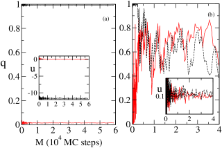
Figure 2: Time evolution of the order parameter $q$ for a single run starting from two independent initial configurations simulated with (a) the Metropolis algorithm and $(b)$ the PT, for $L=20$, $T=1.5$, $D=8.0$, and $K/J=3$. In the insets the time evolution of the total energy per volume $u$ is given for those initial configurations. In contrast with the PT, until $M=6\times 10^{4}$ MC steps the Metropolis algorithm provides a nonergodic simulation.

Next, in Fig. 3 $(a)$ the time evolution of the system simulated via PT with local and non-local exchanges is comapared with the results provided by cluster algorithms. Note that for $\delta>2$ and $M>3\times 10^{4}$ MC steps, the time evolution the PT simulation for $q$ converges to $q\approx 2/3$ (as will be explained later), in agreement with cluster algorithm simulations. A similar behavior is obtained in all cases for the quantity $m$. In Fig. 3 $(b)$ shows the exchange mean probability $p^{*}=\langle\min\{1,\exp[(\beta_{i}-\beta_{j})({\cal H}(\sigma_{i})-{\cal H}(\sigma_{j})]\}\rangle$ juan as a function of $T$ for different distances $\delta$ between replicas and $L=20$. Except for $\delta=1$, the minimum in $p^{*}$ occurs at $T\approx 1.95$, indicating the coexistence between the ferromagnetic phases, paramagnetic rich at spins 0 and a disordered phase, that takes place in the limit of high temperatures BEGMODEL . Our results show that, although non-local exchanges are performed less frequently than local ones, they are fundamental for ensuring an ergodic simulation of the system.

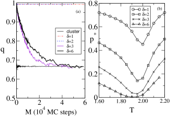
Figure 3: In graph $(a)$ we show the time evolution of the order parameter $q$ simulated by cluster algorithm and PT with exchanges between $i$ and its $i+\delta$th next neighbor replica ($\delta=1,2,3$ and $6$) for $L=20$ and $NR=500$ independent runs. In graph $(b)$ it is shown the mean probability $p^{*}$ versus $T$ for different $\delta$.

Next, we will describe the methodology employed in determining coexistence lines. Their location will be derived from finite size analysis for both the order parameter $q$ and the susceptibility $\chi_{T}$.

Although a discontinuous phase transition is characterized by a jump in the order parameter, the discontinuity takes place only in the thermodynamic limit. For finite systems, not only the order parameter, but also other quantities are described by continuous functions fiore6 ; wang . In such case, the behavior of physical quantities scales with the volume of the system rBoKo ; challa . In Fig. 4, the order parameter $q$ is shown as a function of $D$ for several values of $L$.

Although isotherms present strong dependence on the system size, they intersect one another at the point $D=D^{*}_{0}=8.0000(1)$ and $q\approx 2/3$. As it was explained in Refs. fiore4 ; fiore6 by means of two different reasonings, the point where all isotherms cross is independent of the lattice size. This can be understood recalling that in the regime of low temperatures two ferromagnetic phases ($q\approx 1$) coexist with a paramagnetic phase rich at spins zero ($q\approx 0$) at $D=D^{*}_{0}$, yielding $q\approx 2/3$ for all system sizes. Therefore, the crossing point can be used as a criterion to estimate the transition point. As it will be shown later, the estimate of $D^{*}_{0}$ agrees very well with the value $D^{*}_{\infty}$ obtained from finite size analysis for the susceptibility $\chi_{T}$. In Fig. 4(b), we describe the collapse of all data by the expression $y^{*}=(D-D^{*}_{0})L^{2}$ confirming the dependence on the volume. At low temperatures, the relation between $q$ with the system size $L$ and $D$ is expressed by the following equation fiore6 ; fiore5

$$q=\frac{b+ce^{-{\bar{a}}z}}{1+de^{-{\bar{a}}z}},$$ (2)

where ${\bar{a}}$, $b$, $c$ and $d$ are fitting parameters and $z\equiv D-D^{*}_{0}$. In Fig. 4 (a), continuous lines correspond to the fittings proposed by Eq. (2). The parameter ${\bar{a}}$ scales with the volume, as shown in Fig. 4(c). In the thermodynamic limit $L\rightarrow\infty$, while the quantity ${\bar{a}}$ diverges the order parameter $q$ does not. According to Eq. (2), in the ferromagnetic phase, which occurs in the region $D-D_{0}^{*}<0$, we have that $q\rightarrow c/d$ as $L\rightarrow\infty$. On the other hand, in the paramagnetic phase, which appears for $D-D_{0}^{*}>0$, $q\rightarrow b$ as $L\rightarrow\infty$. For $D=D_{0}^{*}$, we have a jump in $q$, signing a discontinuous phase transition.

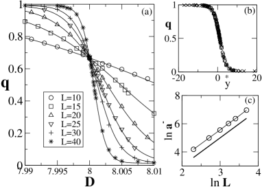
Figure 4: Order parameter per volume $q$ versus $D$ for several values of the system size $L$ for $K/J=3$ and $T=1.5$. Continuous lines correspond to the fittings defined by Eq. (2). In $(b)$ we have a collapse of all data by using the relation $y^{*}=(D-D_{0}^{*})L^{2}$. In $(c)$ we have the log-log plot for the quantity ${\bar{a}}$ as a function of $L$. The straight line has slope $2.00(1)$.

In the second analysis, we determine the transition point by examinating the susceptibility $\chi_{T}=\beta L^{2}(\langle q^{2}\rangle-\langle q\rangle^{2})$. Increasing $D$ towards the coexistence line, one observes a sharp peak in $\chi_{T}$ at $D^{*}_{L}$ for all system sizes, as shown in Fig. 5(a). The deviation between $D^{*}_{L}$ and its asymptotic value $D_{\infty}^{*}$ decays as $L^{-2}$ in a first-order transition rBoKo ; challa . Our results satisfy this asymptotic relation, as it can be seen in Fig. 5 $(b)$. From this law, we have obtained the extrapolated value $D_{\infty}^{*}=8.0000(1)$, which agrees with the estimate $D_{0}^{*}$ obtained previously and also agrees with the result ${\bar{D}}=8.0000(1)$, obtained from a cluster algorithm for the BEG model fiore6 . In Fig. 5 $(c)$ we observe that all curves coalesce to $\chi^{*}=\chi_{T}/L^{2}$ and $y^{*}=(D_{L}^{*}-D_{\infty}^{*})L^{2}$, confirming once again the scaling with the volume.

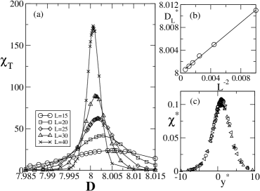
Figure 5: Susceptibility $\chi_{T}$ versus $D$ for several values of the system size $L$, $K/J=3$, and $T=1.5$. In $(b)$, we plot the value of $D=D_{L}^{*}$ in which $\chi_{T}$ is maximum, as a function of $L^{-2}$. In $(c)$ we have a collapse of all data using the relations $\chi^{*}=\chi_{T}/L^{2}$ and $y^{*}=(D-D_{\infty}^{*})L^{2}$.

It is worth emphasizing that when one uses only the Metropolis algorithm to generate the configurations, neither the crossing among isotherms nor accurate finite size analysis for smooth curves become possible, due to the presence of hysteresis effects, as it can be seen in Fig. 1.

In Figs. 6 and 7, we repeat, for $K/J=3.3$ and $T=1.5$, both analysis presented above for determining phase coexistence. From the first procedure, where all isotherms are to be fitted by Eq. (2), the crossing is given by $q\approx 2/3$ and $D_{0}^{*}=8.6032(1)$. This estimate agrees with the value $D_{\infty}^{*}=8.6033(1)$ obtained from finite size analysis for the quantity $\chi_{T}$, as showed in Fig. 7. These estimates, both obtained by using the PT, are in good accordance with the value ${\bar{D}}=8.6032$, obtained by Rachadi and Benyoussef, from cluster algorithms rachadi .

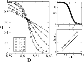
Figure 6: Order parameter per volume $q$ versus $D$ for several values of the system size $L$ for $K/J=3.3$ and $T=1.5$. Continuous lines stand for the fittings defined by Eq. (2). In $(b)$ we have a collapse of all data using the relation $y^{*}=(D-D_{0}^{*})L^{2}$. In $(c)$ we have the log-log plot of ${\bar{a}}$ versus $L$. The straight line has slope $2.00(1)$.

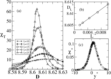
Figure 7: Susceptibility $\chi_{T}$ versus $D$ for several values of the system size $L$, $K/J=3.3$, and $T=1.5$. In $(b)$, we plot the value of $D=D_{L}^{*}$ in which $\chi_{T}$ is maximum, as a function of $L^{-2}$. In $(c)$ we have a collapse of all data using the relations $\chi^{*}=\chi_{T}/L^{2}$ and $y^{*}=(D-D_{\infty}^{*})L^{2}$.

In the last analysis, we show in Fig. 8 numerical results for $K/J=0$ considering $T=0.4$. Fitting all isotherms with Eq. (2), the intersection point turns out to be given by $q\approx 2/3$ and $D_{0}^{*}=1.9968(1)$. The collapse of data using this estimate of $D_{0}^{*}$ confirms again the adequacy of this procedure for the estimation of transition point. Repeating this procedure for $T=0.5$, we verify that all isotherms cross the abscissa $D_{0}^{*}=1.9879(1)$, which is in fair agreement with the estimates $T=0.499(3)$ and ${\bar{D}}=1.992$, predicted by Wang-Landau method pla .

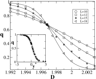
Figure 8: Order parameter per volume $q$ versus $D$ for several values of system size $L$, for $K/J=0$ and $T=0.4$. Continuous lines stand for the fittings defined by Eq. (2). In the inset, we have a collapse of all data using the relation $y^{*}=(D-D_{0}^{*})L^{2}$.

V Conclusion

In this paper, we have applied the parallel tempering method (PT) for the study of first-order transitions. We have considered different regions of the phase diagram of the BEG model, for which usual Metropolis algorithm leads to strong hysteresis at the phase coexistence, providing no reliable estimates of the coexistence lines. On the other hand, by using the PT it was possible to circumvent the free energy barriers and as a consequence hysteretic effects were eliminated. All results obtained via PT allowed us to locate the transition points precisely by means of two techniques, whose estimates agree with those obtained from other procedures, such as cluster algorithms and, in one case, with the Wang-Landau method. Although the agreement between results obtained from PT and cluster algorithms have been shown to be very well, cluster algorithms are more specialized, since each model requires a specific cluster algorithm that takes into account the appropriate transitions. On the other hand, PT is general and can be used, in principle, for any system. We remark that more studies of first-order transitions using the parallel tempering are still required, in order to have a more comprehension of its performance.

VI Acknowledgments

I acknowledge Juan P. Neirotti, Carlos E. I. Carneiro, Silvio R. Salinas, Helmut G. Katzgraber and Renato M. Ângelo, for a critical reading of this manuscript and useful suggestions. This work was partially suported by Fundação de Amparo à Pesquisa do Estado de São Paulo (FAPESP) under Grant No. 06/51286-8.

References

- (1) N. Metropolis, A. W. Rosenbluth, M. N. Rosenbluth and A. H. Teller, J. Chem. Phys. 21, 1087 (1953).
- (2) R. J. Glauber, J. Math. Phys. 4, 294 (1963).
- (3) B. A. Berg and T. Neuhaus, Phys. Lett. B 267, 249 (1991); Phys. Rev. Lett. 68, 9 (1992).
- (4) R. H. Swendsen and J. S. Wang, Phys. Rev. Lett. 58, 86 (1987), U. Wolff, Phys. Rev. Lett 62, 361 (1989).
- (5) M. B. Bouabci and C. E. I. Carneiro, Phys. Rev. B 54, 359 (1996).
- (6) A. Rachadi and A. Benyoussef, Phys. Rev. B 68, 064113 (2003).
- (7) C. E. Fiore and C. E. I. Carneiro, Phys. Rev. E 76, 021118 (2007).
- (8) F. Wang and D. P. Landau, Phys. Rev. Lett. 86, 2050 (2001), Phys. Rev. E 64, 056101 (2001).
- (9) E. Marinari and G. Parisi, Europhys. Lett. 19(6), 451 (1992).
- (10) K. Hukushima and K. Nemoto, J. Phys. Soc. Jpn. 65, 1604 (1996).
- (11) C. J. Geyer, Markov-Chain Monte Carlo maximum Likehood, Comp. Sci. and Stat., p. 156 (1991).
- (12) K. Binder and W. Kob, Glassy Materials and Disordered Solids: An Introduction to their Statistical Mechanics (World Scientific, Singapoure, 2005).
- (13) J. Skolnick and A. Kolinski, Comput. Sci. Eng. 3(9/10), 40 (2001).
- (14) J. P. Neirotti, F. Calvo, D. L. Freeman and J. D. Doll, J. Chem. Phys. 112, 10340 (2000); F. Calvo, J. Chem. Phys. 123, 124106 (2005).
- (15) F. Calvo, J. P. Neirotti, D. L. Freeman and J. D. Doll, J. Chem. Phys. 112, 10350 (2000).
- (16) W. Nadler and U. H. E. Hansmann, Phys. Rev. E 76, 057102 (2007).
- (17) M. Blume, V. J. Emery, and R. B. Griffiths, Phys. Rev. A 4, 1071 (1971), W. Hoston and A. N. Berker, Phys. Rev. Lett. 67, 1027 (1991).
- (18) T. Neuhaus, M. P. Magiera and U. H. E. Hansmann, Phys. Rev. E 76, 045701(R) (2007).
- (19) H. G. Katzgraber, S. Trebst, D. A. Huse and M. Troyer, J. Stat. Mech., P03018 (2006).
- (20) C. Predescu, M. Predescu and C. Ciobanu, J. Chem. Phys. 120, 4119 (2004); J. Phys. Chem, B 109, 4189 (2005).
- (21) C. J. Silva, A. A. Caparica and J. A. Plascak, Phys. Rev. E 73, 036702 (2006).
- (22) M. S. S. Challa, D. P. Landau and K. Binder, Phys. Rev. B 34, 1841 (1986).
- (23) C. Borgs and R. Kotecký, Phys. Rev. Lett. 68, 1734 (1992); J. Stat. Phys. 61, 79 (1990).
- (24) C. E. Fiore, V. B. Henriques and M. J. de Oliveira, J. Chem. Phys. 125, 164509 (2006).
- (25) The expression (2) is derived from Borgs and Koteckỳ theory, where it was shown that at low temperatures the partition function for two or more coexisting phases can be expressed in terms of the metastable free energy of each phase. By taking the derivate of the logarithm of the partition function with respect to , one gets an expression for , as given in Eq. (2). More details can be found in Ref. fiore6 .