Obtaining pressure versus concentration phase diagrams in spin systems from Monte Carlo simulations

Abstract

We propose an efficient procedure for determining phase diagrams of systems that are described by spin models. It consists of combining cluster algorithms with the method proposed by Sauerwein and de Oliveira where the grand canonical potential is obtained directly from the Monte Carlo simulation, without the necessity of performing numerical integrations. The cluster algorithm presented in this paper eliminates metastability in first order phase transitions allowing us to locate precisely the first-order transitions lines. We also produce a different technique for calculating the thermodynamic limit of quantities such as the magnetization whose infinite volume limit is not straightforward in first order phase transitions. As an application, we study the Andelman model for Langmuir monolayers made of chiral molecules that is equivalent to the Blume-Emery-Griffiths spin-1 model. We have obtained the phase diagrams in the case where the intermolecular forces favor interactions between enantiomers of the same type (homochiral interactions). In particular, we have determined diagrams in the surface pressure versus concentration plane which are more relevant from the experimental point of view and less usual in numerical studies.

I Introduction

The importance of numerical simulations in Physics is due to the fact that very few models can be exactly solved. In principle one may directly simulate any model on a computer. Moreover, the Metropolis metr and the Glauber glauber algorithms used in Monte Carlo (MC) simulations are very general and easy to implement. In practice things are not so simple. Near second-order phase transitions the configurations generated by these algorithms present strong temporal correlations (critical slowing down), which prevent an efficient sampling of the configuration space. In addition, hysteresis effects due to metastability prevent a precise location of first-order transition lines.

In the last years, several techniques have been proposed to circumvent these problems such as the reweighting technique by Berg and Neuhaus berg and the simulated tempering by Marinari and Parisi parisi . A different approach is the use of cluster algorithms pioneered by Swendsen and Wang sw and by Wolff wolff . Several studies have shown the efficiency of cluster algorithms in reducing the critical slowing down sw . More recently, it has been shown that the cluster dynamics may practically eliminate metastability in first order phase transitions So far this has been achieved only for the Blume-Emery-Griffiths (BEG) spin-1 model BEGMODEL ; BEG2 , for which a special cluster algorithm has been developed bouabci ; rachadi .

In this paper, we present a simple cluster algorithm that eliminates metastability in first-order phase transitions and combine it to the Sauerwein and de Oliveira (SO) method that allows us to obtain the surface pressure directly from numerical simulations sauerwein . In the original formulation of the SO method, the authors used the Metropolis dynamics to generate the system configurations. However, as explained above, this is not the best choice near phase boundaries. We also introduce a simple procedure to calculate the order parameters and the concentrations of molecules in the neighborhood of a first-order line from numerical simulations.

As an application of our method, we have determined the phase diagrams of the Andelman model for Langmuir monolayers made of chiral molecules. More specifically, we were interested in surface pressure versus concentration phase diagrams, which are more interesting from the experimental point of view. The Andelman model was first studied by using the mean field approach on a bipartite lattice andelman1 . However, X-ray diffraction experiments suggest that the condensed phases of Langmuir monolayers tend to form triangular structures, and not a bipartite lattice as considered by Andelman. In order to be more consistent with the physics of Langmuir monolayers, Pelizzola et al pelizzola have studied the heterochiral case on a two dimensional triangular lattice, using the cluster variation method, and have obtained phase diagrams that are qualitatively different from Andelman’s. We study through MC simulations the remaining homochiral case, and we show that, in contrast with the heterochiral case, the MC and the mean field methods give results that are in good agreement.

This paper is organized as follows: in section 2 we briefly review the Andelman model, in section 3 we present the cluster algorithm and briefly review the Sauerwein de Oliveira method, in section 4 we discuss the numerical results and conclude in section 5.

II Chiral Langmuir monolayers and the Blume-Emery-Griffiths model

Langmuir monolayers are formed by spreading amphiphilic molecules in an air-water interface. Amphiphilic molecules are strongly asymmetric, constituted by two parts with opposite features. The first part—the head—, is hydrophilic. It is made of polar chemical groups and remains on the water. The second part—the tail—, is hydrophobic and made of hydrocarbon chains which remain in the air. When the tail is strongly hydrophobic, so that the molecules are insoluble in water, Langmuir monolayers form a quasi-two dimensional system. This system can be described in terms of the surface pressure and temperature and it displays several phases with different structural properties (see, for instance Ref kaganer ).

A chiral molecule exists in two forms $+$ and $-$, called enantiomers, related by a spatial transformation that involves a change of parity. An important feature of the physics of chiral Langmuir monolayers is the determination of the chiral discrimination, which occurs when the interaction energy between enantiomers with the same chirality is different from the interaction energy of enantiomers with different chirality. When the intermolecular forces favor the attraction between enantiomers of the same species, they are denominated homochiral and they lead to chiral segregation. On the contrary, if the attraction between different enantiomers is favored, they are named heterochiral and they lead to a racemic mixture.

To study the effect of the chirality theoretically, Andelman proposed a simple lattice gas model that can be described by the Hamiltonian pelizzola

$${\cal H}=-\sum_{<i,j>}\sum_{r,s}\epsilon_{rs}N_{r,i}N_{s,j}-\sum_{i}\sum_{s}\mu_{s}N_{s,i},$$ (1)

where the first sum is over nearest-neighbor pairs, the letters $i$ and $j$ denote the sites of a two-dimensional triangular lattice, the letters $r$ and $s$ denote the enantiomer species ($r,s=+$ or $-$), $\epsilon_{rs}$ are the coupling energies ($\epsilon_{++}=\epsilon_{--}$ and $\epsilon_{+-}=\epsilon_{-+}$), $N_{r,i}=0,1$ are the occupation numbers at site $i$, and $\mu_{s}$ is the chemical potential of the species $s$.

This model is equivalent to the Blume-Emery-Griffiths (BEG) spin-1 model BEGMODEL ; BEG2 , as it can be seen by relating the occupation numbers and the spin-1 variables through the relations

$$N_{+,i}=\frac{\sigma_{i}^{2}+\sigma_{i}}{2},\qquad N_{-,i}=\frac{\sigma_{i}^{2}-\sigma_{i}}{2},$$ (2)

where $\sigma_{i}=0,\pm 1$. Thus, $\sigma_{i}=1\quad(-1)$ represents a $+$ ($-$) enantiomer and $\sigma_{i}=0$ a vacancy. In this way, we obtain the BEG Hamiltonian

$${\cal H}=-\sum_{(i,j)}[J\,\sigma_{i}\sigma_{j}+\phi\,\sigma_{i}^{2}\sigma_{j}^{2}]-\sum_{i}[H\sigma_{i}-\Delta\sigma_{i}^{2}],$$ (3)

The case $J>0$ corresponds to the homochiral case (ferromagnetic BEG). When $J<0$, we have the heterochiral one (antiferromagnetic BEG). We will concern ourselves with the homochiral case, since it has not been studied beyond the mean-field approach. The parameters $J,\phi$ depend on the interaction energies $\epsilon_{++}=\epsilon_{--}$ and $\epsilon_{+-}=\epsilon_{-+}$ between nearest-neighbor enantiomers through the formulae

$$J=\frac{1}{2}(\epsilon_{++}-\epsilon_{+-}),$$ (4)

and

$$\phi=\frac{1}{2}(\epsilon_{++}+\epsilon_{+-}).$$ (5)

The fields $H$ and $\Delta$ are related to the chemical potential of the species $+$ and $-$ and they are given by

$${\it H}=\frac{\mu_{+}-\mu_{-}}{2},$$ (6)

and

$$-\Delta=\frac{\mu_{+}+\mu_{-}}{2}.$$ (7)

They are the conjugate parameters of the chiral order parameter and the density of enantiomers defined by

$$M\equiv\left\langle\sum_{i=1}^{V}\sigma_{i}\right\rangle=\;\langle N_{+}\rangle-\langle N_{-}\rangle,$$ (8)

and

$$Q\equiv\left\langle\sum_{i=1}^{V}\sigma_{i}^{2}\right\rangle=\;\langle N_{+}\rangle+\langle N_{-}\rangle,$$ (9)

where the $N_{\pm}$ are the total number of enantiomers $\pm$ and $V=L^{2}$ is the number of lattice sites. In particular, we are interested in determining the concentration of enantiomers $+$ or $-$ ($x_{+}$ or $x_{-}$, respectively) given by

$$x_{\pm}=\frac{\langle N_{\pm}\rangle}{\langle N_{+}\rangle+\langle N_{-}\rangle}=\frac{1}{2}(1\pm\frac{M}{Q})=\frac{1}{2}(1\pm\frac{m}{q}),$$ (10)

where $m=M/V$, $q=Q/V$.

In this work we shall study first-order transitions between concentrated phases where the enantiomers are close to each other (phases $C_{+}$ and $C_{-}$ rich in enantiomers of type $+$ and $-$, respectively) and the so called liquid expanded ($LE$) phases, where there are many vacancies. In the spin-1 language, we shall study transitions between ferromagnetic and paramagnetic phases rich in zero spins.

III Monte Carlo method

III.1 Cluster algorithm

In experiments involving chiral Langmuir monolayers the non chiral contribution to the interaction energy between the enantiomers is usually larger than the chiral one. In our simplified model, this corresponds to choosing the parameter $\phi$ larger than $J$. In this paper, we will consider the ratio $\phi/J=3$. This choice has also been previously made by Andelman andelman1 and Pelizzola et al pelizzola . For $\phi/J=3$, Eq. (3) can be rewritten, up to a constant term, in the following way

$$\beta{\cal H}=-2K\sum_{<i,j>}\delta_{\sigma_{i},\sigma_{j}}+(\bar{\Delta}-2Kz)\sum_{i=1}^{N}\sigma_{i}^{2}-\bar{H}\sum_{i=1}^{N}\sigma_{i},$$ (11)

where we used the following identity $-(\sigma_{i}\sigma_{j}+\sigma_{i}^{2}\sigma_{j}^{2})-2(\sigma_{i}^{2}-1)(\sigma_{j}^{2}-1)\equiv-2\delta_{\sigma_{i},\sigma_{j}}$, $K\equiv\beta J$, $\bar{\Delta}\equiv\beta\Delta$, $\bar{H}\equiv\beta H$, and $z$ is the coordination number. For this Hamiltonian, we propose the following cluster algorithm:

1. Choose randomly a site on the lattice and denote $\sigma_{\rm seed}$ the value of its spin. This is the first spin of the cluster (seed).

2. Choose, with the probability 0.5, one of the two other possible spin values that are different from $\sigma_{\rm seed}$. Call this new value $\sigma_{\rm new}$ (it will remain fixed during the construction of the cluster). For example, if $\sigma_{\rm seed}$ is $+$, $\sigma_{\rm new}$ can be $-$ or $0$.

3. Activate the links between the seed and its nearest neighbors that are equal to $\sigma_{\rm seed}$ with probability $p=1-e^{-2K}$. Each new spin connected to the cluster by an activated link is added to the cluster. Next, we repeat the activation procedure to all the new spins of the cluster. The process stops when all nearest neighbors have been tested and no new spin is accepted. Now, we attempt to change this cluster with spins equal to $\sigma_{\rm seed}$ into a cluster with spins $\sigma_{\rm new}$ (see Fig. 1, for an example of a $+\rightarrow 0$ transition).

4. Evaluate the difference $\delta{\mathcal{H}_{\rm bulk}}={\tilde{\mathcal{H}}_{\rm bulk}}-{\mathcal{H}_{\rm bulk}}$, where $\tilde{\mathcal{H}}_{\rm bulk}$ is the cluster bulk energy (calculated neglecting boundary links) when all spins are equal to $\sigma_{\rm new}$ and $\mathcal{H}_{\rm bulk}$ is the cluster bulk energy when all spins are equal to $\sigma_{\rm seed}$. If $\delta\mathcal{H}_{\rm bulk}\leq 0$, we change all spins in the cluster to $\sigma_{\rm new}$ with probability $P_{\rm flip}(\sigma\rightarrow\tilde{\sigma})=1$. If $\delta\mathcal{H}_{\rm bulk}>0$, we change all spins in the cluster to $\sigma_{\rm new}$ with probability $P_{\rm flip}(\sigma\rightarrow\tilde{\sigma})=\exp(-\beta\delta\cal H_{\rm bulk})$.

To prove that the algorithm satisfies the detailed balance condition we have to consider two types of transitions: $\pm\leftrightarrow\mp$ and $\pm\leftrightarrow 0$. For the first transition our algorithm is equivalent to Wolff’s wolff and for this reason we shall concentrate on transitions of the second type. Let us consider, to exemplify, the transition $+\leftrightarrow 0$. From Eq. (11), we obtain

$$\frac{e^{\beta{\cal H}}}{e^{\beta\tilde{\cal H}}}=\frac{e^{-2K\ell_{++}}}{e^{-2K\tilde{\ell}_{00}}}e^{-\beta\delta{\mathcal{H}_{\rm bulk}}},$$ (12)

where $\ell_{\alpha\gamma}$ is the total number of boundary links that connect sites with spins $\alpha$ inside the cluster and sites with spins $\gamma$ outside the cluster.

The ratio between the transition probability $W_{\sigma\rightarrow\tilde{\sigma}}$ and the reverse transition probability $W_{\tilde{\sigma}\rightarrow\sigma}$ is given by

$$\frac{W_{\sigma\rightarrow\tilde{\sigma}}}{W_{\tilde{\sigma}\rightarrow\sigma}}=\frac{w_{\rm bulk}(1-p)^{\ell_{++}}P_{\rm flip}(\sigma\rightarrow\tilde{\sigma})}{\tilde{w}_{\rm bulk}(1-p)^{\tilde{\ell}_{00}}P_{\rm flip}(\tilde{\sigma}\rightarrow\sigma)}.$$ (13)

The bulk term $w_{\rm bulk}$ is the sum of the probabilities associated with all possible ways of activating links to construct the cluster, the term $(1-p)^{\ell_{++}}$ is the probability of not including in the cluster a nearest neighbor site with occupation variable $\sigma_{\rm seed}$. Analogous comments hold for the transition $W_{\tilde{\sigma}\rightarrow\sigma}$. Clearly, $w_{\rm bulk}=\tilde{w}_{\rm bulk}$ because for each configuration of activated links in $\sigma$ there is a corresponding one in $\tilde{\sigma}$ (see Fig. 1). Recalling the definition of $P_{\rm flip}$, given in step 4 of the algorithm, we see that the ratio of the flipping probabilities is always equal to $\exp(-\beta\delta\mathcal{H}_{\rm bulk})$. Finally, since $1-p=e^{-2K}$ the right hand sides of Eqs. (12) and (13) are equal and this equality implies detailed balance. It is worth mentioning that the algorithm proposed here is a particular case of the cluster algorithm proposed by Bouabci and Carneiro bouabci and later extended by Rachadi and Benyoussef rachadi for other regions of the parameter space.

III.2 The Sauerwein and de Oliveira method

In order to determine the grand canonical potential from Monte Carlo simulations, one usually calculates one of its derivatives and numerically integrate the results. To use this technique one has to know the value of the grand canonical potential at a reference point and then numerically integrate along a path which connects the reference point to the point where one wants to calculate the grand canonical potential. An alternative is the method proposed by Sauerwein and de Oliveira sauerwein that allows one to directly obtain the grand canonical potential from the MC simulation.

In this method, the largest eigenvalue of the transfer matrix is directly evaluated from Monte Carlo simulations. Since in the thermodynamic limit the grand partition function is proportional to the largest eigenvalue of the transfer matrix, its calculation enables us to determine all thermodynamic properties, in particular the surface pressure that is the negative of the grand canonical potential.

In order to explain how to obtain the largest eigenvalue, let us consider a triangular lattice with $V$ sites divided in $N$ successive layers $S_{k}\equiv(\sigma_{1,k},\sigma_{2,k},...,\sigma_{L,k})$ with $L$ spins, $V=L\times N$ (All this applies to the triangular lattice that we use in our paper.). The Hamiltonian may be decomposed in the following way

$${\cal H}=\sum_{k=1}^{N}{\cal H}(S_{k},S_{k+1}),$$ (14)

where due to the periodic boundary conditions $S_{N+1}=S_{1}$. The probability $P(S_{1},S_{2},...,S_{N})$ of a given configuration of the system is given by

$$P(S_{1},S_{2},...,S_{N})=\frac{1}{Z}T(S_{1},S_{2})T(S_{2},S_{3})...T(S_{N},S_{1}),$$ (15)

where $T(S_{k},S_{k+1})\equiv\exp(-\beta{\cal H}(S_{k},S_{k+1}))$ is an element of the transfer matrix $T$ and

$$Z=\rm Tr(\it{T^{N}}),$$ (16)

is the grand-canonical partition function. By using the spectral expansion of the matrix $T$ it is possible to show sauerwein that

$$<\delta_{S_{1},S_{2}}>=\frac{1}{\lambda_{0}}<T(S_{1},S_{1})>.$$ (17)

This expression enables us to calculate the largest eigenvalue $\lambda_{0}$ of the transfer matrix $T$ in terms of the averages $<\delta_{S_{1},S_{2}}>$ and $<T(S_{1},S_{1})>$, where $\delta_{S_{1},S_{2}}=1$ when layers $S_{1}$ and $S_{2}$ are equal and zero otherwise. We use a MC simulation to generate the configurations with which we calculate the averages.

In the specific case of the BEG Hamiltonian in the triangular lattice with $L\times L$ sites, the transfer matrix $T$ of a $n$-layer is given by

$$T(S_{n},S_{n+1})=\exp\{\sum_{k=1}^{L}[K\sigma_{k,n}(\sigma_{k,n+1}+\sigma_{k+1,n}$$

$$+\sigma_{k+1,n+1})+\beta\phi\sigma_{k,n}^{2}(\sigma_{k,n+1}^{2}+\sigma_{k+1,n}^{2}+\sigma_{k+1,n+1}^{2})$$

$$-\bar{\Delta}\sigma_{k,n}^{2}+\bar{H}\sigma_{k,n}]\}.$$ (18)

The grand canonical potential per site in the lattice gas representation (or the free energy in the spin-1 representation) is given by

$$\psi=-\frac{1}{\beta L}\ln\lambda_{0}=-{\cal P},$$ (19)

where ${\cal P}$ is the surface pressure.

IV Numerical results

In this section, we define the following dimensionless quantities:

$$t\equiv k_{B}T/J,\quad D\equiv\Delta/J,\quad h\equiv H/J,\quad\Pi\equiv{\cal P}/J,$$ (20)

where ${\mathcal{P}}$, the surface pressure, is given by Eq. (19).

As a check on the efficiency of the proposed cluster algorithm, we show in Fig. 2 the grand canonical potential $\psi$ versus the chemical potential $D$ for $h=0$ and $t=0.8$. We considered a very low temperature, because in this case hysteresis effects are very strong. In Fig. 2 we compare the performances of the Metropolis and the cluster algorithm on a triangular lattice with periodic boundary conditions and linear dimension $L=30$. To evaluate $\psi$ and to estimate its statistical error after equilibrating the systems we have used $5\times 10^{4}$ Monte Carlo steps divided into $1000$ independent runs. Note that with the Metropolis algorithm the system is trapped in metastable states and even after millions of MC steps it does not undergo a transition to the stable phase. This does not happen with the cluster algorithm because the system is able to easily pass from one phase to the other. The efficiency of the algorithm allows us to determine first-order transition lines with high precision and the good quality of the data enables us to perform very precise finite size analysis.

In principle it is possible to determine the transition point using the free energy. As it can be seen in Fig. 2, there is a kink in the free energy as a function of $D$ at the transition point $D_{L}^{*}$. One can then perform a finite size analysis to obtain $D_{\infty}^{*}$. However, it is simpler and more efficient to analyze the susceptibility whose finite size behavior is well known for both first and second-order phase transitions. After determining $D_{\infty}^{*}$ we use the SO method at this point to calculate the surface pressure. In first-order phase transitions, the surface pressure, which is proportional to the negative of the grand canonical potential, does not have a finite size behavior as simple as the susceptibility. As a function of the system size, the surface pressure saturates quickly. Thus, the values of the surface pressure that we use in our graphs come from the largest lattices that we have simulated.

The susceptibility is defined as $\chi_{t}=L^{2}(\langle m^{2}\rangle-\langle|m|\rangle^{2})/t$, where the magnetization $m=\sum_{i}\sigma_{i}/V$. For a fixed system size $L$, maintaining $t$ and $h$ fixed, and increasing $D$ towards the coexistence line, one observes a peak in the susceptibility at $D_{L}^{*}$, as seen in Fig. 3, where the lines were drawn only to guide the eye. In the thermodynamic limit, this peak becomes a delta-function singularity. According to Refs. rBoKo ; challa , the deviation of $D_{L}^{*}$ from its asymptotic value $D_{\infty}^{*}$ decays as $L^{-2}$, in agreement with our results, shown in the inset of Fig. 3 . From this law, we have obtained the extrapolated value $D_{\infty}^{*}=12.0000(1)$.

In order to understand this result let us perform an exact zero temperature calculation of the transition point $D_{L}^{*}$. At zero temperature the free energy $F=U-TS=U\equiv<{\mathcal{H}}>$, where ${\mathcal{H}}$ is given in Eq. (3). The system chooses the phase that minimizes the energy $U$. At $T=0$, for small values of $D$ all spins are $+1$ if $h>0$ or $-1$ if $h<0$. If $D$ is large enough, the energy is minimized when all spins are $0$. The transition line is obtained by equating the energies in the ferromagnetic (condensed) phase with all $\sigma_{i}=+$ (or $-$) and in the paramagnetic (liquid expanded) phase with all $\sigma_{i}=0$. Taking into account Eq. (3), with $\phi=3J$, and the definitions given in Eq. (20), we calculate the energy $U_{\pm}$ of the ferromagnetic phases and the energy $U_{0}$ of the paramagnetic phase

$$U_{\pm}=VJ(-12\mp h+D)\,;\quad U_{0}=0.$$ (21)

The equation $U_{\pm}=U_{0}\Leftrightarrow D=12\pm h$ gives the transition lines between the ferromagnetic and paramagnetic phases. The equation $U_{+}=U_{-}\Leftrightarrow h=0$ gives the transition line between the two ferromagnetic phases (this holds for $D\leq 12$, for $D>12$ the systems is in the paramagnetic phase). All these transition lines are represented in Fig. 4 that gives the phase diagram of the Langmuir monolayer in the plane of the chemical potentials $h\times D$ (Recall that $hJ=H=(\mu_{+}-\mu_{-})/2$ and $DJ=\Delta=(-\mu_{+}-\mu_{-})/2$.). The circles are the results of Monte Carlo simulations performed at $t=2.4$. The error bars are smaller than the circles. It is interesting to remark that in the temperature interval relevant for Langmuir monolayers the zero temperature calculations give practically the same results as the MC simulations and the mean-field calculations for the transition lines. In Langmuir monolayers language, for $h=0$ and low values of $D$ (higher chemical potentials), we have the condensed phase characterized by a $1:1$ mixture of the two enantiomers. For higher values of $D$ a transition from the condensed phase, rich in enantiomers $\pm 1$, to the phase poor in enantiomers, the liquid expanded phase, takes place. When the chemical potential of the species are different ($h\neq 0$), we have larger fraction of enantiomers $+$ $(-)$ whenever $h>0$ $(h<0)$, and in the limit of $h>>0$ $(<<0)$ the solution only contains the enantiomer $+$ $(-)$.

Another procedure for locating the phase transition consists in determining the crossing point of the $q$ versus $D$ isotherms for different system sizes. As showed in the Ref. fiore4 , the crossing point is independent of the lattice size and properly identifies the transition, as shown in Fig. 5. We shall present below an independent derivation of this important result based on the work of Borgs and Kotecký rBoKo .

For $h=0$ all curves of $q$ versus $D$ cross at $D^{*}=12.0000(1)$ and $q\approx 2/3$ for this value of $D$. This criterion for estimating the value of $D$ for which the phase transition takes place agrees very well with the finite size analysis of the susceptibility $\chi_{t}$ that we have discussed above. For $h\neq 0$, two phases coexist at the point $D_{h}^{*}$ which now depends on $h$ and all isotherms cross at $q\approx 0.5$. We remark that if single flip algorithms are used to generate the dynamics, one will not be able to determine the crossing of the curves due to hysteresis effects.

More relevant from the point of view of Langmuir monolayers, and other physical systems involving mixture of molecules, are the surface-pressure versus concentration diagrams. But before discussing this phase diagram we will describe our procedure to fit the curves in Fig. 5 and to obtain the $V\rightarrow\infty$ limit of $q$ and $m$ that are used to determine the concentration $x_{+}$ (see Eq. (10)). Since the simulated system is finite, the calculated quantities will be affected by finite size effects. As mentioned previously, in the last years, the finite size theory of first order phase transitions has been studied extensively for quantities, such as the specific heat and the susceptibility. There are fewer studies for the dependence on the system size of quantities like the magnetization or the concentration of molecules gupta ; borgs94 . In the following, we propose a method to determine the concentrations of the phases that coexist directly from the numerical simulations. The first step consists in noting that $q\times D$ (or $m\times D$) isotherms can be fitted by the equation

$$q=\frac{b+ce^{-a\,\delta D}}{1+de^{-a\,\delta D}},$$ (22)

where $a$, $b$, $c$ and $d$ are fitting parameters and $\delta D\equiv D-D^{*}_{\infty}$. We are going to show below that $a$ depends on the system size $L$ and the temperature $T$. An analogous expression can be written down for the order parameter $m$. The expression above was inspired by the work of Borgs and Kotecký rBoKo , where it is shown that at low temperatures the partition function for two coexisting phases can be written as

$$Z=[e^{-\beta f_{1}(\beta,h)V}+e^{-\beta f_{2}(\beta,h)V}](1+e^{-L/L_{0}}),$$ (23)

where $h$ is the magnetic field (our system also depends on the crystal field $D$), $L_{0}$ is a constant of the order of the infinite volume correlation length and $f_{i}$ is a metastable free energy for the phase $i$ ($i=1\;\mbox{or}\;2$).

In our system, for $h=0$ three phases coexist at the triple point ($D_{\infty}^{*}=12$). Thus, we expect the sum of three exponentials instead of two as in Eq. (23). We have assumed that all three exponentials have the same weight (we shall use our results to check this point). In the neighborhood of the triple point

$$Z\approx e^{-\beta Vf_{0}}+e^{-\beta Vf_{+}}+e^{-\beta Vf_{-}},$$ (24)

where the $f_{i}=f_{i}(\beta,h,D)$, $i=0,\pm$, are respectively the metastable free energies of the paramagnetic and ferromagnet phases. Away from the coexistence curve, only the $f_{i}$ associated with the correct phase remains and becomes the free energy of the system ($Z=\exp(-\beta Vf_{i})$ ).

The parameters $m$ and $q$ are given by

$$q=-\frac{1}{\beta V}\frac{\partial\log Z}{\partial D},\quad m=-\frac{1}{\beta V}\frac{\partial\log Z}{\partial h}.$$ (25)

For $h=0$, $f_{+}=f_{-}\equiv f_{\pm}$. Taking into account this fact and Eqs. (24) and (25), we can write the parameter $q$ as

$$q\approx\frac{(\partial f_{0}/\partial D)e^{-\beta Vf_{0}}+2(\partial f_{\pm}/\partial D)e^{-\beta Vf_{\pm}}}{e^{-\beta Vf_{0}}+2e^{-\beta Vf_{\pm}}}.$$ (26)

At the triple point $f_{0}^{*}=f_{\pm}^{*}$, where $f_{i}^{*}\equiv f_{i}(\beta,h=0,D=D_{\infty}^{*})$, $i=0,\pm$ and the exponentials in Eq. (26), which contain the only dependence on the lattice size, cancel out and we obtain

$$q^{*}\equiv q(\beta,0,D_{\infty}^{*})\approx\frac{1}{3}\left[\left.\frac{\partial f_{0}}{\partial D}\right|_{D=D_{\infty}^{*}}+\left.2\frac{\partial f_{\pm}}{\partial D}\right|_{D=D_{\infty}^{*}}\right].$$ (27)

This is the reason why the $q\times D$ curves for different lattice sizes cross at the same point. The crossing point provides another method do locate the phase boundaries.

Our calculations are performed at low temperatures. In mean-field, the temperatures are measured in units of the coordination number $z$. For the triangular lattice, $z=6$. Our MC temperature $t=2.4$ is equivalent to a $t=0.4$ mean-field temperature. We can use the exact zero temperature energies given in Eq. (21) to estimate the derivatives in Eq. (27). Recalling that $f_{i}=U_{i}/VJ$, $i=0,\pm$, at $t=0$, we obtain $\partial f_{0}/\partial D=0$ and $\partial f_{\pm}/\partial D=1$. Thus, at the triple point $q^{*}\approx 2/3$ which is the result that we obtain in Fig. 5.

An analogous demonstration holds for the case $h\neq 0$, where $Z$ is the sum of two exponentials as in Eq. (23). The factor $2$ in Eq. (29) is replaced by $1$ and the crossing of the $q\times D$ curves occurs at the point $D\approx 0.5$.

In the curves plotted in Fig. 5, $D$ varies in the interval $[11.994,12.006]$ which is very narrow. It is possible in this case to expand the $f_{i}=f_{i}(\beta,h=0,D)$, $i=0,\pm$, around the triple point,

$$f_{i}=f_{i}^{*}+f_{i}^{\,\prime*}\,\delta D+{\mathcal{O}}((\delta D)^{2}),$$ (28)

where $\delta D\equiv D-D_{\infty}^{*}$, $f_{i}^{*}\equiv f_{i}(\beta,h=0,D=D_{\infty}^{*})$ and $f_{i}^{\,\prime*}\equiv(\partial f_{i}/\partial D)|\{D=D_{\infty}^{*}\}$, for $i=0,\pm$,

$$q\approx\frac{f_{0}^{\,\prime*}\,e^{-\beta Vf_{0}^{\,\prime*}\,\delta D}+2f_{\pm}^{\,\prime*}\,e^{-\beta Vf_{\pm}^{\,\prime*}\,\delta D}}{e^{-\beta Vf_{0}^{\,\prime*}\,\delta D}+2e^{-\beta Vf_{\pm}^{\,\prime*}\,\delta D}},$$ (29)

which has the same form as Eq. (22) after we divide the numerator and the denominator by $\exp(-\beta Vf_{0}^{\,\prime*}\,\delta D)$.

In Fig. 5 the symbols stand for the values of $q$ obtained from the numerical simulations and the solid lines are fits of the points using Eq. (22) by minimizing the $\chi^{2}$ merit function press . In order to perform the fittings we used the Levenberg-Marquardt method that is well described in Ref. press , where one can also find the subroutines that are necessary to implement the method. These subroutines return the variances of the fitting parameters and the quality of the fitting. A few words about the implementation of the subroutines is in order. Our fitting function Eq. (22) contains exponentials whose arguments may become very large. In order to avoid numerical overflow it is convenient to use the asymptotic values of $q$ when $|\delta D|$ becomes too large. Define, for example, $q\equiv b$ for $\delta D>30$ and $q\equiv c/d$ for $\delta D<-30$. Of course, the number $30$ is rather arbitrary. Non-linear fittings depend on a good initial guess of the fitting parameters. One may proceed as follows. Note that $b=q(D\rightarrow\infty)$ and $c/d=q(D\rightarrow-\infty)$. Since in the simulations the $D$ interval is finite, instead of taking the $|D|\rightarrow\infty$ limit we use the values of $q$ in our data set associated with the largest and the smallest values of $D$. Call them $q_{+}$ and $q_{-}$, respectively and put $b\approx q_{+}$, $c/d\approx q_{-}$. Next define $q^{*}\equiv q(D=D_{\infty}^{*})$ and $q_{1}\equiv q(D=D_{1})$, where $D_{1}<D_{\infty}^{*}$, is chosen in the region where the graph $q\times D$ has already started to curve down. It is simple to solve the fitting parameters in terms of these quantities.

$$a=\frac{1}{D_{\infty}^{*}-D_{1}}\log\left|\frac{(q_{1}-q_{+})(q_{-}-q^{*})}{(q_{-}-q_{1})(q^{*}-q_{+})}\right|,$$

$$b=q_{+},\quad c=\frac{q_{-}(q^{*}-q_{+})}{q_{-}-q^{*}},\quad d=\frac{q^{*}-q_{+}}{q_{-}-q^{*}}.$$ (30)

With this choice for the initial parameters, the convergence of the fitting routine is very fast and the quality of the fitting is very good (the factor $Q$ that measures the goodness-of-fit press is close to $1$). In Tables 1 and 2 the errors of the parameters are the square roots of the variances (standard deviations) that are returned by the fitting routines.

The fitting parameters for the curves in Fig. 5 are given in Table 1. Now we can check the equal weight hypothesis for the exponentials. For $h=0$ the two condensed phases $C_{\pm}$ have the same free energy and two of the three exponentials are identical, as we discussed above. The $q\times D$ curves in Fig. 5 are in the vicinity of the triple point, so we expect that $d\approx 2$. This is the result that we obtain (see Tables 1 and 2 for the magnetization $m$).

For $h\neq 0$, there is the coexistence of two phases ($LE$ and $C_{+}$ or $C_{-}$). Near the transition we have the sum of two exponentials with the same weight, as in Eq. (23). We have checked that $d\approx 1$ near the transition line, as it was expected.

Comparing Eqs. (22) and (26) we note that the parameter $a$ that appears in the exponent should be proportional to the system volume. A $\log(a)\times\log(L)$ plot gives the straight line $\log(a)=A+B\log(L)$ with $A=-0.87(2)$ and $B=1.990(6)$ for table 1; and $A=-0.88(2)$ and $B=1.993(5)$ for table 2. Thus, as expected, the constant $a$ scales with the volume of the system.

The values of $q$ for the condensed and liquid expanded phases are calculated by taking the $L\rightarrow\infty$ limit in Eq. (22). The condensed phases occur in the region $D-D_{\infty}^{*}<0$ and for this reason $q\rightarrow c/d$ as $L\rightarrow\infty$. The liquid expanded phase occurs in the region $D-D_{\infty}^{*}>0$ and $q\rightarrow b$ as $L\rightarrow\infty$. The curves for $m\times D$ are very similar to the curves $q\times D$ in Fig. 5 and can be also be fitted by an expression analogous to Eq. 22. Having calculated $q$ and $m$, we obtain $x_{+}$ through the expression $x_{+}=(1+|m|/q)/2$. The use of $|m|$ instead of $m$ is due to technical reasons (see sections 2.3.3 and 2.3.4 in Ref. binder ). As a consequence, the magnetization is small but not zero when $h=0$. This introduces a small distortion in the diagram of Fig. 6 near $x_{+}=0.5$, but symmetry arguments guarantee that $m=0$ when $h=0$ and the coexistence curve passes through the point with $x_{+}=0.5$ (filled circle in Fig. 6).

The $h>0$ half side of the diagram $h\times D$ is mapped onto the right hand side of the surface-pressure versus concentration diagram ($x_{+}>0.5$) whereas $h<0$ corresponds to the $x_{+}<0.5$ concentration range. As mentioned above, $h=0$ implies that the fraction of enantiomers $+$ and $-$ are equal and in the coexistence of the three phases, one has $x_{+}=0.5$. From the point of view of homochiral Langmuir monolayers, the chiral segregation takes place, in contrast to the heterochiral case, in which one has a racemic mixture. The surface pressure of a 1:1 mixture of enantiomers is higher than the pressure for pure enantiomers. This feature is verified in experiments in which the chiral segregation occurs kaganer . Unfortunately, to date few experiments have been performed covering the whole range of concentrations, usually they are restricted to the 1:1 mixture and the pure cases. For comparison, we have also plotted in Fig. 6 the results obtained from the mean field technique.

In contrast to the heterochiral case, for which the mean field results disagree with those obtained from the cluster variational method, in the homochiral case the accordance between mean field and the numerical simulations is very good.

V Conclusions

In this paper, we present an efficient way for determining phase diagrams from numerical simulations. To illustrate it, we have considered a simple model that describes the behavior of homochiral Langmuir monolayers, which is equivalent to the BEG model. It is worth mentioning that although we have interpreted the phase diagrams obtained here in terms of Langmuir monolayers, similar phase diagrams are obtained when one uses the BEG model to describe a mixture of two distinct species with vacancies. The use of a cluster algorithm that eliminates metastability in first order phase transitions allows us to precisely locate the first-order transitions lines. To determine the surface pressure we used the method proposed by Sauerwein and de Oliveira in which the surface pressure is determined directly from the numerical simulations without the necessity of performing numerical integrations. The fitting procedure proposed in this paper to determine the concentrations, based on the work of Borgs and Kotecký rBoKo , is easy to implement and uses all information contained in the order parameter curve. It seems to improve on the usual finite size analysis for the magnetization near first-order transition lines in that it does not present “overshooting” effects gupta ; borgs94 and both $m$ and $q$ present a monotonic behavior as a function of $L$, but this point has to be further investigated by increasing the statistics. The elimination of metastability also enables us to use the crossing of the curves $q\times D$ (or $m\times D$) for different lattice sizes as a criterium for locating the phase boundaries. This usually cannot be done due to hysteresis effects. Finally, we remark that our approach is general and it can be used for any spin model. In systems for which a cluster algorithm is not available, we can use other techniques, such as the multicanonical approach berg or the simulated tempering parisi to generate the dynamics.

Figure 1: Example of a possible cluster transition. The heavy lines are the activated links.

Figure 2: Grand canonical potential $\psi/J$ versus $D$ across the first-order line for $L=30$, $h=0$ and $t=0.8$. The first graph refers to the Metropolis algorithm and the second to the cluster algorithm. The symbol $\circ$ ($\times$) indicates increasing (decreasing) $D$. The symbols are larger than the error bars.

Figure 3: Susceptibility $\chi_{t}$ versus $D$ for several values of system size $L$, $h=0$ and $t=2.4$. In the inset, we plotted the value of $D$ for which the susceptibility is maximum ($D_{L}^{*}$) versus $L^{-2}$.

Figure 4: Phase diagram in the space of the chemical potentials $h$ versus $D$. The symbols $C_{+}$ and $C_{-}$ denote the condensed phases rich in enantiomers $+$ and $-$, respectively, and $LE$ is the liquid expanded phase. The solid line is the $t=0$ calculation which practically coincides with the mean field result. The circles are from MC simulations.

Figure 5: Order parameter $q$ versus $D$ for $h=0$, $t=2.4$ and several system sizes $L$. In the inset, a collapse of all curves by plotting $q$ versus $z=(D-D_{\infty}^{*})*L^{2}$.

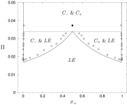
Figure 6: Surface pressure $\Pi$ versus concentration $x_{+}$ phase diagram obtained by numerical simulations (circles) and mean field (lines).

L	a	b	c	d
24	233.2(9)	0.0173(7)	1.983(8)	2.000(8)
30	363(1)	0.0166(4)	1.986(2)	2.004(9)
36	521(2)	0.0161(4)	1.99(1)	2.01(1)
42	708(3)	0.0160(3)	1.99(1)	2.00(1)
48	925(4)	0.0160(3)	1.99(1)	2.00(1)
54	1168(6)	0.0160(3)	1.98(1)	2.00(1)
60	1.45(1)$\times 10^{3}$	0.0165(7)	1.98(1)	2.00(2)

Table 1: Values of the fitting parameters obtained from the $q\times D$ curves in Fig. 4 ($t=2.4$ and $h=0$). The numbers between brackets are the uncertainties in the last digits.

L	a	b	c	d
24	233.4(9)	0.0047(6)	1.943(8)	1.998(8)
30	364(1)	0.0036(2)	1.943(9)	1.998(9)
36	523(2)	0.0029(1)	1.94(1)	2.00(1)
42	711(3)	0.0025(1)	1.94(1)	2.00(1)
48	930(4)	0.0022(1)	1.94(1)	1.99(1)
54	1175(6)	0.00200(9)	1.93(1)	1.99(1)
60	1.45(1)$\times 10^{3}$	0.0018(3)	1.93(2)	1.99(2)

Table 2: Values of the fitting parameters obtained from the $m\times D$ curves for $t=2.4$ and $h=0$.

References

- (1) N. Metropolis, A. W. Rosenbluth, M. N. Rosenbluth, A. H. Teller and E. Teller, J. Chem. Phys. 21, 1087 (1953).
- (2) R. J. Glauber, J. Math. Phys. 4, 294 (1963).
- (3) B. A. Berg and T. Neuhaus, Phys. Lett. B 267, 249 (1991); Phys. Rev. Lett. 68, 9 (1992).
- (4) E. Marinari and G. Parisi, Europhys. Lett. 19(6), 451 (1992).
- (5) R. H. Swendsen and J. S. Wang, Phys. Rev. Lett. 58, 86 (1987).
- (6) U. Wolff, Phys. Rev. Lett 62, 361 (1989).
- (7) M. Blume, V. J. Emery, and R. B. Griffiths, Phys. Rev. A 4 , 1071 (1971).
- (8) W. Hoston and A. N. Berker, Phys. Rev. Lett. 67, 1027 (1991).
- (9) M. B. Bouabci and C. E. I. Carneiro, Phys. Rev. B 54, 359 (1996).
- (10) A. Rachadi and A. Benyoussef, Phys. Rev. B 68, 064113 (2003).
- (11) R. A. Sauerwein and M. J. de Oliveira, Phys. Rev. B, 52, 3060 (1995).
- (12) D. Andelman, J. Am. Chem. Soc, 111, 6536 (1989).
- (13) A. Pelizzola, M. Pretti and E. Escalas, J. of Chem. Phys. 112, 8126 (2000).
- (14) C. Borgs and R. Kotecký, J. Stat. Phys. 61 79 (1990) and Phys. Rev. Lett. 68 1734 (1992).
- (15) M. S. S. Challa, D. P. Landau and K. Binder, Phys. Rev. B 34, 1841 (1986).
- (16) V. M. Kaganer, H. Möhwald, and P. Dutta, Rev. Mod. Phys. 71, 779 (1999).
- (17) C. E. Fiore, V. B. Henriques and M. J. de Oliveira, J. Chem. Phys. 125, 164509 (2006).
- (18) S. Gupta, A. Irbäck and M. Ohlsson, N. Phys. 409, 663 (1993), S. Gupta and A. Irbäck, N. Phys. 30, 861 (1993).
- (19) C. Borgs, P. E. L. Rakow and S. Kappler, J. of Phys. I, 4, 1027 (1994).
- (20) W. H. Press, B. P. Flannery, S. A. Teukolsky and W. T. Vetterling, Numerical Recipes: The Art of Scientific Computing (Cambridge Univ. Press, New York, 1987).
- (21) K. Binder and D. W. Heermann, Monte Carlo Simulation in Statistical Physics (Springer-Verlag, New York Berlin Heidelberg, 1992).