Hierarchical mean-field approach to the $J_{1}$-$J_{2}$ Heisenberg model on a square lattice

Abstract

We study the quantum phase diagram and excitation spectrum of the frustrated $J_{1}$-$J_{2}$ spin-1/2 Heisenberg Hamiltonian. A hierarchical mean-field approach, at the heart of which lies the idea of identifying relevant degrees of freedom, is developed. Thus, by performing educated, manifestly symmetry preserving mean-field approximations, we unveil fundamental properties of the system. We then compare various coverings of the square lattice with plaquettes, dimers and other degrees of freedom, and show that only the symmetric plaquette covering, which reproduces the original Bravais lattice, leads to the known phase diagram. The intermediate quantum paramagnetic phase is shown to be a (singlet) plaquette crystal, connected with the neighbouring Néel phase by a continuous phase transition. We also introduce fluctuations around the hierarchical mean-field solutions, and demonstrate that in the paramagnetic phase the ground and first excited states are separated by a finite gap, which closes in the Néel and columnar phases. Our results suggest that the quantum phase transition between Néel and paramagnetic phases can be properly described within the Ginzburg-Landau-Wilson paradigm.

I Introduction

One of the primary goals of modern condensed matter physics is the characterization of strongly correlated quantum systems. A large class of such materials is represented by frustrated antiferromagnets, which are believed to exhibit a variety of novel states of matter at sufficiently strong coupling. Growing experimental evidence indicates that layered materials such as ${\rm Li_{2}VO(Si,Ge)O_{4}}$ Millet , ${\rm VOMoO_{4}}$ Carretta and ${\rm BaCdVO(PO_{4})_{2}}$ Nath can be adequately described by an antiferromagnetic Heisenberg model with frustrating next- and next-next-nearest neighbor interactions. As a result, the study of low-dimensional magnets and their frustration-driven quantum phase transitions have attracted a lot of theoretical attention in the last decade Sachdev_1999 ; Lhuillier_2004 .

A paradigmatic system, illustrating the effects of frustrating couplings, is the spin-$1/2$ Heisenberg model on a square lattice with competing nearest ($J_{1}$), and next-nearest ($J_{2}$) neighbor antiferromagnetic (AF) interactions ($J_{1}$-$J_{2}$ model). Despite numerous analytical and numerical efforts, its phase diagram, which exhibits a two sublattice Néel AF, quantum paramagnetic, and a four sublattice columnar AF states, continues to stir certain controversy (for a review of recent achievements, see Ref. Lhuillier_2004, ). While existence of the Néel-ordered phase at small frustration ratio $J_{2}/J_{1}$, and of the columnar AF state at large $J_{2}/J_{1}$ is widely established, properties of the intermediate non-magnetic phase, which occurs around the maximum frustration value $J_{2}/J_{1}=1/2$, are still under debate. Particularly, the correlated nature of the intermediate state and the kind of quantum phase transition separating it from the Néel state, attract most attention. Various methods have been recently applied to characterize the quantum paramagnetic phase, such as Green’s function Monte Carlo Sorella_2000 ; Sorella_2001 ; Leeuwen_2000 , coupled cluster methods Richter_2008 , series expansions Singh_1999 and field-theoretical methods Takano_2003 ; Kotov_1999 ; Parola_2006 . As a result, several possible candidate ground states were proposed, namely: spin liquid Sorella_2001 , preserving translational and rotational symmetries of the lattice, as well as various lattice symmetry breaking phases, out of which the dimer Kotov_1999 ; Sachdev_1991 , and the plaquette resonating valence bond phases Sorella_2000 are worth mentioning.

Not surprisingly, the nature of the quantum phase transition separating the Néel-ordered and quantum paramagnetic phases is also under scrutiny. The most dramatic, and at the same time original, scenario Sachdev_2004 is believed to violate the Ginzburg-Landau-Wilson paradigm of phase transitions Landau_1999 which revolves around the concept of an order parameter. Such point of view is based on the observation that there are different spontaneously broken symmetries in the Néel and quantum paramagnetic phases, which thus cannot be connected by a group-subgroup relation. The former, of course, breaks the $SU(2)$ invariance of the Hamiltonian and lattice translational symmetry $T$ Manousakis_1989 ; cluster , but preserves the four-fold rotational symmetry of the square $C_{4}$. On the other hand, the paramagnetic phase is known to restore the spin-rotational symmetry and is believed to break $T$ and $C_{4}$, due to spontaneous formation of dimers along the links of the lattice Sachdev_1991 ; Kotov_1999 . It follows then, that these two phases can not be joined by the usual Landau second-order critical point. This phase transition can either be of the first-order Sirker_2006 (the latest coupled cluster calculations Richter_2008 , however, seem to rule out this possibility), or represent an example of a second order critical point, which cannot be described in terms of a bulk order parameter, but rather in terms of emergent fractional excitations (spinons), which become deconfined right at the critical point Sachdev_2004 .

However, evidence regarding the structure of the non-magnetic phase is quite controversial. Indeed, the results of spin-wave calculations Kotov_1999 , large-$N$ expansions Sachdev_1991 , and calculations using the density matrix renormalization group combined with Monte-Carlo simulations Leeuwen_2000 are believed to indicate the emergence of a dimer order. On the other hand, Monte-Carlo Sorella_2000 and coupled cluster calculations Richter_2008 , and analytical results Takano_2003 seem to support the presence of $C_{4}$ symmetry (plaquette-type ordering) in the paramagnetic phase. In the absence of a reliable numerical or analytical proof of existence of any particular order in the non-magnetic region, there is no apparent reason to believe in the exotic deconfined quantum criticality scenario. Although there apparently exists numerical evidence Sandvik_2007 , at the moment of writing the authors are unaware of a local Hamiltonian in space dimensions larger than one, rigorously proven to exhibit the type of quantum critical point discussed in Ref. Sachdev_2004, . Interestingly, it was demonstrated in Ref. Batista_2004, that a two-dimensional (2D) lattice model can possess a first order quantum critical point, which exhibits deconfined excitations.

All in all, the complexity of methods used to infer properties of the paramagnetic phase and the variety of different conclusions have created a certain degree of confusion. Our goal in the present paper is to try to clarify some of this controversy by proposing a controlled and manifestly symmetry preserving method, geared to computing ground state properties of the $J_{1}$-$J_{2}$ model. Our approach is based on the recently proposed systematic methodology to investigate the behavior of strongly coupled systems Ortiz_2003 , whose main idea consists of identifying relevant degrees of freedom and performing an educated approximation, called the hierarchical mean-field (HMF), to uncover the phase diagram and other properties of the system of interest. In a future work these ideas will be coupled to a new, variational with respect to the energy, renormalization group approach, which thus adapts to the concept of relevant degrees of freedom.

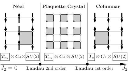
Figure 1: A schematic phase diagram of the $J_{1}$-$J_{2}$ model, summarizing our results. In each phase we show spontaneously broken (framed symbols) and unbroken symmetries (usual symbols). The translational invariance is broken along both directions in the Néel and paramagnetic phases, and only along the $y$–direction in the columnar phase. This fact is indicated by the subscripts $xy$ and $y$ after $T$. Conclusions regarding the order of the phase transition, separating Néel and plaquette crystal phases, as well as symmetries of various phases, are based upon extrapolation of our results towards the thermodynamic limit.

In the present work we construct HMF approximations for the $J_{1}$-$J_{2}$ model. The crux of our method is the identification of a plaquette (spin cluster $2\times 2$ or even larger $4\times 4$ (superplaquette) symmetry-preserving cluster) as the relevant elementary degree of freedom, which captures necessary quantum correlations to represent essential features of the phase diagram. The importance of this degree of freedom was realized only recently in the present context Takano_2003 , and somewhat earlier in connection with $SU(4)$ spin-orbital Mila_2000 , and Hubbard Altman_2002 models. Besides being variational, our formalism has the attractive feature of preserving fundamental lattice point symmetries and the $SU(2)$ symmetry of the Hamiltonian, by utilizing the Schwinger boson-type representation and Racah algebra technology. Remarkably, such simple mean-field calculation already yields all known results, concerning the phase diagram of the $J_{1}$-$J_{2}$ model, with a good accuracy, namely: existence of a Néel-ordered phase with antiferromagnetic wavevector $(\pi,\pi)$ and spin-wave type excitations for $J_{2}/J_{1}\lesssim 0.42$, a non-magnetic intermediate gapped phase, separated by a second order quantum phase transition, and a first order transition point, which is characterized by the discontinuous disappearance of the energy gap and connects the paramagnetic state with the columnar antiferromagnetic phase at $(\pi,0)$ and $(0,\pi)$ for $J_{2}/J_{1}\gtrsim 0.66$.

We emphasize that our investigation primarily focuses on the symmetry analysis of the various phases. Out of many possible coarse graining scenarios, such as covering of the 2D lattice with plaquettes, dimers and crosses, only the $C_{4}$-symmetry preserving plaquette (or superplaquette) covering (which reproduces the original Bravais lattice) displays the correct phase diagram. In particular, the intermediate paramagnetic phase is shown to be a plaquette crystal, which preserves spin and lattice rotational symmetries. For all other scenarios, including dimerized (bond-ordered) phases, we were unable to reproduce all known quantum phase transition points of the model.

We notice that the HMF coarse graining procedure leads to an explicit breaking of a particular translational symmetry. As a result, one can not draw rigorous conclusions on the order of the phase transitions, based solely on a fixed coarse graining. Nevertheless, it is still possible to make some predictions, using a finite-size scaling of the relevant degree of freedom towards the thermodynamic limit, where the effects associated with coarse graining should disappear.

Next two sections are devoted to the formulation of the HMF approach. Then, we present results of our calculations and close the paper with a discussion. Our main conclusions are summarized in Fig. 1, which emphasizes symmetry relations between different phases of the model.

II The plaquette degree of freedom

We consider the spin-$1/2$ antiferromagnetic Heisenberg model with frustrated next-nearest neighbor interactions $J_{2}$, defined on a 2D bipartite lattice with $N$ sites:

$$H=J_{1}\sum_{\langle i,j\rangle}{\bm{S}}_{i}\cdot{\bm{S}}_{j}+J_{2}\sum_{\langle\langle i,j\rangle\rangle}{\bm{S}}_{i}\cdot{\bm{S}}_{j}.$$ (1)

As mentioned already in the Introduction, we choose the plaquette, Fig. 2, as our elementary degree of freedom. Then, assuming that $N$ is chosen appropriately, the entire lattice can be covered with such plaquettes in a sub-exponentially Mila_2000 ($\sim 2^{\sqrt{N}}$) large number of ways.

Aiming at illustrating the main idea of the method, in this section we consider in detail only the symmetric covering of the lattice with $2\times 2$ plaquettes, which preserves the $C_{4}$ lattice symmetry, see Fig. 3, although later the displaced covering (Fig. 4), which breaks $C_{4}$ down to $C_{2}$ (two-fold symmetry axis), and the case of larger plaquettes (superplaquettes, Fig. 13) will be analyzed as well.

It is convenient to take as a basis the states

$$|a\rangle=|l_{1}l_{2}LM\rangle,$$ (2)

where ${\bm{l}}_{1}={\bm{S}}_{1}+{\bm{S}}_{4}$ and ${\bm{l}}_{2}={\bm{S}}_{2}+{\bm{S}}_{3}$ are total spins of the plaquette diagonals, while ${\bm{L}}={\bm{l}}_{1}+{\bm{l}}_{2}$ is the total spin of the entire plaquette and $M$ is its $z$-component. In this basis the Hamiltonian of a single plaquette,

$$H_{\Box}=J_{1}\bigl{(}{\bm{S}}_{1}+{\bm{S}}_{4}\bigr{)}\bigl{(}{\bm{S}}_{2}+{\bm{S}}_{3}\bigr{)}+J_{2}\bigl{(}{\bm{S}}_{1}\cdot{\bm{S}}_{4}+{\bm{S}}_{2}\cdot{\bm{S}}_{3}\bigr{)}$$ (3)

is diagonal with eigenvalues

$$\epsilon_{l_{1}l_{2}L}= \frac{J_{1}}{2}\bigl{[}L\bigl{(}L+1\bigr{)}-l_{1}\bigl{(}l_{1}+1\bigr{)}-l_{2}\bigl{(}l_{2}+1\bigr{)}\bigr{]}+$$

$$+ \frac{J_{2}}{2}\bigl{[}l_{1}\bigl{(}l_{1}+1\bigr{)}+l_{2}\bigl{(}l_{2}+1\bigr{)}-3\bigl{]}.$$ (4)

We note that the basis of Eq. (2) is a natural one and allows us to explicitly label states with corresponding representations of $SU(2)$.

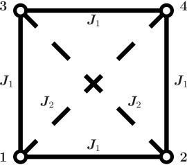
Figure 2: A single $2\times 2$ plaquette has each vertex occupied by a $S=1/2$ spin. The diagonal spins interact through a Heisenberg term of strength $J_{2}$, while nearest neighbor spins interact with strength $J_{1}$.

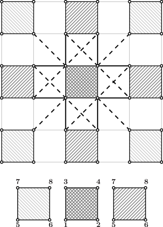
Figure 3: Symmetric covering of the 2D lattice with $2\times 2$ plaquettes. Each plaquette is connected to 4 nearest and 4 next-nearest neighbors.

The next step is to establish how a plaquette couples to the rest of the system. In Fig. 3 we show the symmetric plaquette covering of the 2D lattice. In the figure the vertices of every non-central plaquette are similarly labeled by the numbers $5,6,7,8$, and total spins of diagonals are ${\bm{l}}_{3}={\bm{S}}_{5}+{\bm{S}}_{8}$ and ${\bm{l}}_{4}={\bm{S}}_{6}+{\bm{S}}_{7}$. In the uncoupled basis matrix elements of the inter-plaquette interaction are:

$$\bigl{(}H_{\rm int}^{\sigma} \bigr{)}^{a_{1}^{\prime}a_{2}^{\prime}}_{a_{1}a_{2}}=\sum_{LM}\bigl{\langle}\lambda_{1}^{\prime}\lambda_{2}^{\prime},LM|H_{\rm int}^{\sigma}|\lambda_{1}\lambda_{2},LM\bigr{\rangle}\times$$ (5)

$$\times\bigl{\langle}L_{1}^{\prime}M_{1}^{\prime}L_{2}^{\prime}M_{2}^{\prime}|L_{1}^{\prime}L_{2}^{\prime}LM\bigr{\rangle}\bigl{\langle}L_{1}M_{1}L_{2}M_{2}|L_{1}L_{2}LM\bigr{\rangle},$$

where $\sigma=1$ ($\sigma=2$) corresponds to the nearest (next-nearest) neighbor interaction, $L_{1}$,$L_{2}$ ($L_{1}^{\prime}$,$L_{2}^{\prime}$) represent initial (final) angular momenta of the two plaquettes and ${\bm{L}}={\bm{L}}_{1}+{\bm{L}}_{2}$ is their total angular momentum. In this equation we have introduced the notations $\lambda_{1}=\{l_{1}l_{2}L_{1}\}$, $\lambda_{2}=\{l_{3}l_{4}L_{2}\}$ and $a_{i}=\{\lambda_{i}M_{i}\}$, and similarly for the primed indices. Because each plaquette has 4 nearest neighbors and 4 next-nearest neighbors (see Fig. 3), the symmetrized next-nearest neighbor interaction may be written as:

$$\bigl{\langle} \lambda_{1}^{\prime}\lambda_{2}^{\prime},LM|H_{\rm int}^{2}|\lambda_{1}\lambda_{2},LM\bigr{\rangle}=J_{2}\rho_{L_{1}L_{2}}^{L_{1}^{\prime}L_{2}^{\prime}}(L)\times$$ (6)

$$\times \biggl{(}\!S_{3}^{\lambda_{1}^{\prime}\lambda_{1}}S_{6}^{\lambda_{2}^{\prime}\lambda_{2}}\!\!+S_{1}^{\lambda_{1}^{\prime}\lambda_{1}}S_{8}^{\lambda_{2}^{\prime}\lambda_{2}}\!\!+S_{2}^{\lambda_{1}^{\prime}\lambda_{1}}S_{7}^{\lambda_{2}^{\prime}\lambda_{2}}\!\!+S_{4}^{\lambda_{1}^{\prime}\lambda_{1}}S_{5}^{\lambda_{2}^{\prime}\lambda_{2}}\!\biggr{)}.$$

while the symmetrized nearest neighbor plaquette interaction has the form:

$$\bigl{\langle}\lambda_{1}^{\prime} \lambda_{2}^{\prime},LM|H_{\rm int}^{1}|\lambda_{1}\lambda_{2},LM\bigr{\rangle}=J_{1}\rho_{L_{1}L_{2}}^{L_{1}^{\prime}L_{2}^{\prime}}(L)\times$$ (7)

$$\times\bigl{[}\bigl{(}S_{1}^{\lambda_{1}^{\prime}\lambda_{1}}+S_{4}^{\lambda_{1}^{\prime}\lambda_{1}}\bigr{)}\bigl{(}S_{6}^{\lambda_{2}^{\prime}\lambda_{2}}+S_{7}^{\lambda_{2}^{\prime}\lambda_{2}}\bigr{)}+$$

$$\qquad+\bigl{(}S_{2}^{\lambda_{1}^{\prime}\lambda_{1}}+S_{3}^{\lambda_{1}^{\prime}\lambda_{1}}\bigr{)}\bigl{(}S_{5}^{\lambda_{2}^{\prime}\lambda_{2}}+S_{8}^{\lambda_{2}^{\prime}\lambda_{2}}\bigr{)}\bigr{]}+$$

$$\qquad+2\bigl{\langle}\lambda_{1}^{\prime}\lambda_{2}^{\prime},LM|H_{\rm int}^{2}|\lambda_{1}\lambda_{2},LM\bigr{\rangle},$$

In Eqs. (6) and (7) the symbols $S_{n}^{\lambda^{\prime}\lambda}=\langle\lambda^{\prime}\|S_{n}\|\lambda\rangle$ denote reduced matrix elements of the $n$-th spin operator, and:

$$\rho_{L_{1}L_{2}}^{L_{1}^{\prime}L_{2}^{\prime}}(L)=\frac{1}{4}(-1)^{L+L_{2}^{\prime}+L_{1}}\left\{\begin{array}[]{ccc}L_{1}^{\prime}&L_{2}^{\prime}&L\\ L_{2}&L_{1}&1\end{array}\right\},$$

where $\{\cdots\}$ are Wigner $6j$ symbols (or Racah coefficients) Edmonds_1957 .

Let us now identify the plaquette degree of freedom with a Schwinger boson which creates a specific state of the plaquette. Then, the Hamiltonian of Eq. (1) in the plaquette basis can be expressed as:

$$H= \sum_{i,a}\epsilon_{a}\gamma_{ia}^{\dagger}\gamma_{ia}+\sum_{\langle ij\rangle}\bigl{(}H_{\rm int}^{1}\bigr{)}^{a_{1}^{\prime}a_{2}^{\prime}}_{a_{1}a_{2}}\gamma_{ia_{1}^{\prime}}^{\dagger}\gamma_{ja_{2}^{\prime}}^{\dagger}\gamma_{ia_{1}}\gamma_{ja_{2}}+$$

$$+\sum_{\langle\langle ij\rangle\rangle}\bigl{(}H_{\rm int}^{2}\bigr{)}^{a_{1}^{\prime}a_{2}^{\prime}}_{a_{1}a_{2}}\gamma_{ia_{1}^{\prime}}^{\dagger}\gamma_{ja_{2}^{\prime}}^{\dagger}\gamma_{ia_{1}}\gamma_{ja_{2}},$$ (8)

where the operator $\gamma_{ia}^{\dagger}$ creates a boson on site $i$ of the plaquette lattice (which contains $N_{\Box}=N/4$ sites) in the state, denoted by an index $a$, running through the entire single-plaquette Hilbert space (of dimension $2^{4}=16$) and the summation is performed over doubly repeated dummy indices. The unphysical states are eliminated by enforcing the local constraint $\sum_{a}\gamma_{ia}^{\dagger}\gamma_{ia}=1$. In what follows, we impose periodic boundary conditions on the plaquette lattice.

The bosonic operators $\gamma_{ia}$ define the hierarchical language Ortiz_2003 for our problem. It will be used in the next section, where we develop an approximation scheme for diagonalizing the Hamiltonian of Eq. (8).

III Hierarchical mean-field approximation

As it follows from Eq. (4), the lowest single-plaquette state has the energy $\epsilon_{1100}/4=-J_{1}/2+J_{2}/8$ per spin, which, when $J_{2}=0$, gives only the energy of a classical 2D antiferromagnet. Thus, it is necessary to take into account the interaction term in Eq. (8).

The HMF approximation is a mean-field approach, performed on the relevant degrees of freedom. In the present section we discuss only the simplest one – a Hatree-Fock like (HF) approximation. A possible way to include fluctuation corrections is presented in Appendix B. The HF approximation introduces the mixing of single-plaquette states which minimizes the total energy of the system and is based on a canonical transformation among the bosons, which we will restrict to be uniform (plaquette independent):

$$\gamma_{ia}=R_{a}^{n}\Gamma_{in}.$$ (9)

The real matrix $R$ satisfies canonical orthogonality and completeness relations:

$$R_{a}^{n}R_{a}^{n^{\prime}}=\delta_{nn^{\prime}};\,\,\,R_{a}^{n}R_{a^{\prime}}^{n}=\delta_{aa^{\prime}}$$

A translationally invariant variational ansatz for the ground state (vacuum) is a boson condensate in the lowest HF single-particle energy state ($n=0$):

$$|{\rm HF}\rangle=\prod_{i}\Gamma_{i0}^{\dagger}|0\rangle,$$ (10)

and since it has one boson per plaquette, there is no need to impose the Schwinger boson constraint in the calculation.

Minimizing the total energy with respect to $R$, we arrive at the self-consistent equation:

$$\biggl{\{}\epsilon_{a}\delta_{aa^{\prime}}+\sum_{\sigma}z_{\sigma}\bigl{(}H_{\rm int}^{\sigma}\bigr{)}^{aa_{1}}_{a^{\prime}a_{2}}R_{a_{1}}^{0}R_{a_{2}}^{0}\biggr{\}}R_{a^{\prime}}^{n}=\varepsilon_{n}R_{a}^{n},$$ (11)

where $z_{1}=z_{2}=4$ are the nearest- and next-nearest coordination numbers. The ground state energy (GSE) per spin is then given by the expression:

$$\frac{E_{0}}{N}=\frac{\langle{\rm HF}|H|{\rm HF}\rangle}{N}=\frac{1}{8}\biggl{(}\varepsilon_{0}+\sum_{a}\epsilon_{a}\bigl{(}R_{a}^{0}\bigr{)}^{2}\biggr{)},$$ (12)

with $\varepsilon_{0}$ being the lowest eigenvalue of Eq. (11).

Another fundamental quantity to compute is the polarization of spins within a plaquette:

$$\langle{\rm HF}|S_{in}^{z}|{\rm HF}\rangle=\left(S_{n}^{z}\right)_{a^{\prime}a}R^{0}_{a^{\prime}}R^{0}_{a},$$

where $n=1,\dots,4$ is the spin index, and the matrix elements (determined from the Wigner-Eckart theorem) are:

$$\left(S_{n}^{z}\right)_{a^{\prime}a}=\langle l_{1}^{\prime}l_{2}^{\prime}L^{\prime}M^{\prime}|S_{n}^{z}|l_{1}l_{2}LM\rangle=$$ (13)

$$= (-1)^{L+L^{\prime}+1}\delta_{MM^{\prime}}\frac{\langle 10LM|1LL^{\prime}M\rangle}{\sqrt{2L^{\prime}+1}}\langle l_{1}^{\prime}l_{2}^{\prime}L^{\prime}||S_{n}||l_{1}l_{2}L\rangle.$$

This enables us to define the staggered and collinear (along $x$ and $y$ axes) magnetizations:

$$M_{\rm stag} =(1/4)\langle{\rm HF}|S_{1}^{z}+S_{4}^{z}-S_{2}^{z}-S_{3}^{z}|{\rm HF}\rangle;$$ (14)

$$M_{\rm col}(x,y) =(1/4)\langle{\rm HF}|S_{1}^{z}-S_{4}^{z}+S_{2,3}^{z}-S_{3,2}^{z}|{\rm HF}\rangle.$$

Notice the extreme simplicity of the HMF approximation. The reason why it is able to realize meaningful results is that the plaquette degree of freedom seems to contain the main correlations defining the physics behind the Hamiltonian of Eqs. (1), and (8). To avoid confusion, we emphasize that the HF approximation and the fluctuation theory of Appendix B are physically (and obviously mathematically) different from the spin-wave or canonical Schwinger-Wigner boson mean-field approach to spin systems Auerbach_1994 . In particular, we make no assumption about the underlying ground state, thus allowing for an interplay of various quantum phases. Moreover, it will be demonstrated, that the collective excitation spectra in each phase consistently reflect spontaneously broken symmetries, unlike the usual Schwinger boson case Auerbach_1994 , in which one obtains gapped excitations.

IV Ground state properties and excitation spectrum of the model

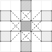
Figure 4: The displaced plaquette covering. Notice that the $C_{4}$ symmetry is broken down to $C_{2}$.

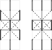
Figure 5: Connectivity of the dimer lattice for symmetric (right panel) and displaced dimer coverings (left panel). The rotational $C_{4}$ symmetry is lowered to $C_{2}$ in both cases.

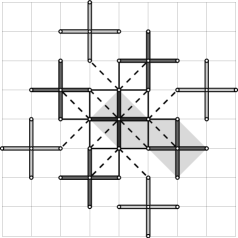
Figure 6: Covering of the lattice with crosses – arrays of five spins. Since one cross cannot form a singlet, it is necessary to double the unit cell, as indicated by the gray shading. This choice of a degree of freedom clearly preserves the $C_{4}$ symmetry, but the resulting lattice breaks it.

Our choice of the plaquette as an elementary degree of freedom remains unjustified at this point. In order to show its relevance we applied the analysis of two previous sections to several other coarse grainings (besides the symmetric plaquette covering, case (a), shown in Fig. 3): (b) superplaquette (spin cluster $4\times 4$) degree of freedom, covering the lattice in such a way that $C_{4}$ is preserved (see Appendix A for details); (c) displaced plaquette covering of the lattice, Fig. 4; (d) symmetric and displaced dimer coverings, shown respectively in right and left panels of Fig. 5; (e) cross degree of freedom, Fig. 6. One should observe that symmetries of the original Bravais lattice are preserved only in cases (a) and (b). In cases (c) and (d) the lattice rotational symmetry $C_{4}$ is lowered to $C_{2}$. Case (e) is special in the sense that an isolated degree of freedom does not possess a singlet ground state. The information about a particular configuration is encoded in matrix elements of $H_{\rm int}^{\sigma}$, whose calculation is elementary. Other equations, presented in Secs. II and III, retain their form.

For each of the above cases we iteratively solve Eq. (11) and compute the GSE (12), and staggered and collinear magnetizations (14). The main message, which we would like to convey in this section is that only the plaquette degree of freedom (of any size) is relevant for constructing the phase diagram of the Hamiltonian of Eq. (1).

IV.1 Symmetry preserving plaquette configurations

Let us focus first on cases (a) and (b), i.e. symmetry-preserving coverings of the lattice with plaquette, Fig. 3, and superplaquette degrees of freedom. The resulting GSE as a function of $J_{2}/J_{1}$ is shown in Fig. 7. One immediately observes a level-crossing at $J_{2}^{c2}\approx 0.67J_{1}$, indicating the first-order transition and a second-order quantum critical point at $J_{2}^{c1}\approx 0.42J_{1}$, which is supported by a jump of the second order derivative $d^{2}E_{0}/dJ_{2}^{2}$, Fig. 8. Both Néel and columnar phases are characterized by spontaneously broken $SU(2)$ symmetry. The former exhibits a nonvanishing staggered magnetization, $M_{\rm stag}$, while the latter has nonzero collinear magnetization along the $x$-direction, $M_{\rm col}(x)$. Both order parameters become zero in the paramagnetic phase, suggesting that $SU(2)$ is restored. These results are summarized in Fig. 9, from which it also follows that the phase transition at $J_{2}^{c1}$ is continuous, while $J_{2}^{c2}$ corresponds to a first-order transition point. We remind, in this connection, that our approach does not explicitly break the spin rotational symmetry, thus allowing for the treatment of competing ground states.

As expected, considering a larger elementary degree of freedom – superplaquette – leads to a significant improvement of the GSE and reduction of the magnetization, due to larger quantum fluctuations. The finite-size scaling (insets in Figs. 7 and 9), using these two sizes ($2\times 2$ and $4\times 4$), indicates that $E_{0}(J_{2}=0)/N\to-0.64J_{1}$ and $M_{z}(J_{2}=0)\to 0.39$ in the thermodynamic limit, a satisfying result for a HF approximation, which completely ignores fluctuations (these numbers should be compared with well-known results of Monte-Carlo simulations Ceperly_1989 : $E_{0}/N\approx-0.67J_{1}$ and $M_{z}\approx 0.31$).

Figure 7: Ground state energy per spin computed at the HF level for the $2\times 2$ and $4\times 4$ plaquette elementary degrees of freedom. The inset shows finite-size scaling in the AF phase at $J_{2}=0$.

Figure 8: Second-order derivative $d^{2}E_{0}/dJ_{2}^{2}$ for the $2\times 2$ and $4\times 4$ plaquette degrees of freedom. The discontinuity at $J_{2}/J_{1}\approx 0.42$ is indicative of a second-order quantum phase transition. In the inset we present finite-size scaling for the jump $g\equiv\left(J_{1}d^{2}E_{0}/NdJ_{2}^{2}\right)_{J_{2}^{c1}-0}^{J_{2}^{c1}+0}$.

Figure 9: Staggered magnetization, $M_{\rm stag}$, for $J_{2}\leq J_{2}^{c1}$ and collinear magnetization along the $x$-direction, $M_{\rm col}(x)$, for $J_{2}\geq J_{2}^{c2}$ (for the $2\times 2$ and $4\times 4$ plaquette degrees of freedom), computed at the HF level. Notice the continuous phase transition at $J_{2}/J_{1}\approx 0.42$ and a first order transition at $J_{2}/J_{1}\approx 0.68$ ($2\times 2$) and $J_{2}/J_{1}\approx 0.66$ ($4\times 4$). The inset shows finite-size scaling of $M_{z}$ at $J_{2}=0$.

Next, we discuss in more detail symmetry properties of the various phases in Figs. 7, 9. At all values of $J_{2}\leq J_{2}^{c2}$, the lattice translational symmetry $T$ is broken cluster , but the rotational $C_{4}$ symmetry is preserved. For $J_{2}\leq J_{2}^{c1}$ this corresponds to a Néel-type long-range order with spontaneously broken $SU(2)$. At large values $J_{2}\geq J_{2}^{c2}$, we observe the columnar ordering, which spontaneously breaks $C_{4}$ down to $C_{2}$, and $SU(2)$, but partially (i.e., along one direction) restores the lattice translational symmetry. We present a more detailed discussion of the spatial symmetries later in this section. In the intermediate region $J_{2}\in(J_{2}^{c1},J_{2}^{c2})$ the spin $SU(2)$ rotational symmetry is restored. In this paramagnetic phase the ground state wavefunction is a tensor product of individual plaquette ground states (with quantum numbers $l_{1}=l_{2}=1$, $L=M=0$):

$$|1100\rangle=\frac{1}{2\sqrt{3}}\biggl{[} 2\bigl{(}|\uparrow_{1}\uparrow_{4}\downarrow_{2}\downarrow_{3}\rangle+|\downarrow_{1}\downarrow_{4}\uparrow_{2}\uparrow_{3}\rangle\bigr{)}-$$

$$-\bigl{(}|\uparrow_{1}\downarrow_{4}\uparrow_{2}\downarrow_{3}\rangle+|\uparrow_{1}\downarrow_{4}\downarrow_{2}\uparrow_{3}\rangle+$$ (15)

$$\,\,\,\,\,\,\,\,+|\downarrow_{1}\uparrow_{4}\uparrow_{2}\downarrow_{3}\rangle+|\downarrow_{1}\uparrow_{4}\downarrow_{2}\uparrow_{3}\rangle\bigr{)}\biggr{]}.$$

This ground state necessarily breaks the lattice translational symmetry, but preserves $C_{4}$. In fact, the paramagnetic region on the phase diagram of Figs. 7 and 9 is a trivial plaquette crystal: a set of non-interacting plaquettes, because the expectation value of the plaquette interaction (see Eq. (8)) in the singlet state $\prod_{i}\gamma^{\dagger}_{i,1100}|0\rangle$ vanishes. An analogous situation is realized when the superplaquette is chosen as an elementary degree of freedom: the paramagnetic phase is a crystal of superplaquettes. It is interesting to note that in Ref. Sorella_2000, a “plaquette resonating-valence-bond state”, exactly equal to (15), has been proposed. However, later Sorella_2001 the intermediate phase was argued to be a spin liquid, i.e., a state that preserves the lattice translational symmetry.

In order to learn about spatial symmetries in various phases, we compare magnitudes of the several lattice symmetry-breaking observables proposed in the literature. We consider the following three, introduced in Ref. Richter_2008, (in the notation of that paper):

$$F_{1}= \frac{1}{N}\sum_{x,y}(-1)^{x}{\bm{S}}_{x,y}{\bm{S}}_{x+1,y};$$

$$F_{2}= \frac{1}{N}\sum_{x,y}{\bm{S}}_{x,y}\bigl{(}{\bm{S}}_{x+1,y}-{\bm{S}}_{x,y+1}\bigr{)};$$

$$F_{4}= \frac{1}{N}\sum_{x,y}{\bm{S}}_{x,y}\bigl{[}(-1)^{x}{\bm{S}}_{x+1,y}+(-1)^{y}{\bm{S}}_{x,y+1}\bigr{]},$$

where indices $x,y$ specify a spin in the 2D lattice. The operator $F_{4}$ probes the plaquette ordering, which preserves the lattice rotational symmetry, while $F_{1}$ and $F_{2}$ correspond to the columnar ordering. We note, however, that $F_{1}$ is already non-zero for an isolated plaquette (or superplaquette). These functions can be combined in the complex “order parameter”, introduced in Ref. Sachdev_2004, . Here we show details of the calculation of functions $F_{1,2,4}$ for the plaquette degree of freedom, case (a), and only present the result for $F_{4}$ for the superplaquette case (b). In the plaquette representation the above operators are written as:

$$F_{1}= \frac{1}{N}\sum_{i,j}\bigl{[}\bigl{(}{\bm{S}}_{1;i,j}{\bm{S}}_{2;i,j}+{\bm{S}}_{3;i,j}{\bm{S}}_{4;i,j}\bigr{)}-$$

$$\,\quad\qquad-\bigl{(}{\bm{S}}_{2;i,j}{\bm{S}}_{5;i+1,j}+{\bm{S}}_{4;i,j}{\bm{S}}_{7;i+1,j}\bigr{)}\bigr{]};$$

$$F_{2,4}= \frac{1}{N}\sum_{i,j}\bigl{[}\bigl{(}{\bm{S}}_{1;i,j}\mp{\bm{S}}_{4;i,j}\bigr{)}\bigl{(}{\bm{S}}_{2;i,j}\mp{\bm{S}}_{3;i,j}\bigr{)}\pm$$ (16)

$$\,\quad\qquad\pm\bigl{(}{\bm{S}}_{2;i,j}{\bm{S}}_{5;i+1,j}+{\bm{S}}_{4;i,j}{\bm{S}}_{7;i+1,j}\mp$$

$$\,\,\qquad\qquad\mp{\bm{S}}_{3;i,j}{\bm{S}}_{5;i,j+1}\mp{\bm{S}}_{4;i,j}{\bm{S}}_{6,i,j+1}\bigr{)}\bigr{]}.$$

In this equation the indices $i,j$ are coordinates of a plaquette in the lattice.

Figure 10: HF ground state expectation values of the symmetry-breaking perturbations, given by Eq. (16), plotted as functions of $J_{2}/J_{1}$ for the plaquette and superplaquette degrees of freedom. Due to the unbroken $C_{4}$ symmetry in the Néel and paramagnetic phases, values of $F_{4}$ are twice larger than the corresponding values of $F_{1}$, except in the columnar phase, where $C_{4}$ is spontaneously broken down to $C_{2}$. The inset shows finite-size scaling for $F_{4}$ for three values of $J_{2}/J_{1}$: $0$ (circles), $0.504$ (triangles) and $0.997$ (rhombs).

Figure 11: The two lowest excitation energies taken at the center of the plaquette Brillouin zone. The main panel shows the self-consistent solution to Bogoliubov’s equations, while the inset corresponds to the time-dependent Gross-Pitaevskii equation (weak coupling). Since wavefunctions of collective excitations in the Néel and columnar phases have different symmetries, there are level crossings in the non-magnetic phase (cusps in the plot).

Expectation values of the functions Eq. (16) in the HF ground state are shown in Fig. 10. Both phase transition points $J_{2}^{c1}$ and $J_{2}^{c2}$ are clearly seen from this plot. All functions change continuously across the second-order critical point $J_{2}^{c1}$ and jump at the first-order transition point $J_{2}^{c2}$. Except in the columnar phase the values of $F_{4}$ are everywhere exactly twice larger than those of $F_{1}$, which is an indication of the unbroken four-fold rotational symmetry of the lattice in these regions. In the columnar phase, on the other hand, this symmetry is broken and the above relation does not hold. While in the Néel and columnar phases nonlocal terms in Eq. (16) are important, in the paramagnetic state the only contribution to either expectation value comes from isolated plaquettes (local terms in Eq. (16)), or superplaquettes. This observation is consistent with properties of the ground state in the non-magnetic phase, discussed earlier in this section.

As mentioned in the Introduction, any choice of degree of freedom breaks explicitly the lattice translational symmetry $T$, with the result that links in the lattice become inequivalent. Indeed, the functions of Eq. (16), defined on the links, have non-zero values even in the AF phase at $J_{2}=0$. However, this effect vanishes in the thermodynamic limit (i.e., as the size of the degree of freedom is increased). The finite-size scaling for $F_{4}(J_{2}/J_{1})$ is presented in the inset to Fig. 10. The three extrapolated values: $F_{4}(0)=-0.075$, $F_{4}(0.504)=-0.245$ and $F_{4}(0.997)=-0.004$, suggest that the “link-wise” translational invariance is restored in the thermodynamic limit in the Néel and columnar phases, but not in the plaquette crystal phase. Moreover, the value of the jump $g\equiv\frac{J_{1}d^{2}E_{0}}{NdJ_{2}^{2}}\bigr{|}_{J_{2}^{c1}-0}^{J_{2}^{c1}+0}$, extrapolated to the thermodynamic limit (see inset to Fig. 8) remains finite: $g(J_{2}^{c1})=-1.006$. In other words, these results imply that the critical point $J_{2}^{c1}$ corresponds to the usual Landau second-order phase transition.

IV.2 Excitations in the plaquette crystal phase

Until now we have considered only ground-state properties of the model Eq. (1). However, low-lying excited states are also of considerable interest. In particular, the paramagnetic phase is known to have gapped excitations, while Néel and columnar phases exhibit Goldstone modes. Thus, the phase transition points $J_{2}^{c1}$ and $J_{2}^{c1}$ must be accompanied by the opening of a gap in the excitation spectrum: the former in a continuous and the latter in a discontinuous fashion. In Appendix B we present a particular method to obtain the collective spectrum of the system. The main idea of this approximation is borrowed from the Bogoliubov-Fetter theory of superfluidity Fetter_1972 . Namely, assume that on each plaquette the majority of Schwinger bosons form a condensate in an appropriately chosen lowest energy state and neglect fluctuations in the number of condensed particles. We note, however, that due to the Schwinger boson constraint, this quantity has the meaning of a probability to find a given plaquette in the lowest energy HF state, rather than the number of particles. Nevertheless, we will call it the condensate fraction $n_{0}$, which, in principle, should be determined self-consistently, and is a measure of the applicability of the entire approximation: it should satisfy the inequality $|n_{0}-1|\ll 1$. Once the condensation part is separated from $\gamma_{ia}$, what remains describes fluctuation corrections to the HF ground state. These fluctuations have rather strong effects near the phase transition points, leading to the modification of $J_{2}^{c1}$ to a $\lambda$-point and its considerable shift. The value of $J_{2}^{c2}$ also changes, but much less significantly. These facts imply that our approximation breaks down near the phase transition points. Indeed, in Appendix B it is shown that close to the transition, the condensate is strongly suppressed. However, deep in each phase $n_{0}\sim 0.9$, thus allowing us to draw conclusions about general properties of the collective spectrum.

Figure 12: HF ground state energy per spin for the displaced plaquette and cross (upper panel), and dimer (lower panel) coverings.

The complete summary of the results is given in Appendix B, here we only present the most interesting one: The gap in the excitation spectrum as a function of $J_{2}/J_{1}$. Although we focus only on case (a) ($2\times 2$ plaquette), the superplaquette degree of freedom can be considered in a similar manner. The gap always occurs in momentum space at ${\bm{k}}=0$, which reflects translational invariance of the plaquette lattice. Below we focus only on this point in the plaquette Brillouin zone. In fact, there are $16-1=15$ collective branches and only some of them become gapless in the phases with spontaneously broken $SU(2)$. However, in the paramagnetic phase all branches develop a gap. In Fig. 11 we show the energy gap $\Delta(J_{2})=\omega({\bm{k}}=0,J_{2})$ for the two lowest excitation branches in a system of $100\times 100$ plaquettes, which approximates well the thermodynamic limit. The main panel shows results of the self-consistent solution of Bogoliubov’s equations. The inset compares it with the solution of the time-dependent Gross-Pitaeveskii equation (28), which corresponds to the weak-coupling approximation. In the Néel and columnar phases there are two spin wave-type Goldstone modes, both of which acquire a gap in the paramagnetic phase, at $J_{2}^{c1}$ and $J_{2}^{c2}$. However, as it follows from Fig. 11, positions of these points change from their HF values to: $J_{2}^{c1}\approx 0.33J_{1}$ and $J_{2}^{c2}\approx 0.65J_{1}$. The critical point $J_{2}^{c1}$ was obtained by extrapolation of the staggered magnetization curve (Fig. 16) to zero, while the first-order point $J_{2}^{c2}$ by extrapolating the two GSE curves in Fig. 14 until intersection. The single-plaquette physical picture, discussed previously in connection with the paramagnetic phase, remains valid, e.g. the condensation occurs again in the plaquette state $|1100\rangle$. Using this observation and symmetries of the matrix elements $\bigr{(}H_{\rm int}^{\sigma}\bigr{)}^{a^{\prime}b^{\prime}}_{ab}$, one can rigorously show the existence of a gap in the non-magnetic region. In fact, we can say, that it is a property of our HMF approximation, rather than a numerical evidence.

IV.3 Other degrees of freedom

Finally, we comment on the results for cases (c)-(e), which, contrary to the configurations considered before, explicitly break lattice rotational symmetry, see Figs. 4-6. The corresponding GSEs are shown in Fig. 12. In contrast to the previously considered scenarios, these cases give qualitatively wrong phase diagrams. Indeed, if we cover the lattice with displaced plaquettes or crosses, there exists no classical spin configuration, which gives the long-range Néel order. On the other hand, such configuration exists for the columnar state. For the displaced plaquette covering the low-$J_{2}$ phase $J_{2}\leq J_{2}^{c2}$ is an $SU(2)$ singlet, and spatially is a set of non-interacting plaquettes (notice the coincidence of $2\times 2$–plaquette energies in the paramagnetic phases of Figs. 7 and 12). Thus, the phase transition to the columnar state is of the first-order. For the cross covering, on the other hand, $SU(2)$ is explicitly broken for all values of $J_{2}$, but since the columnar phase partially restores the lattice translational invariance, it is again separated from the non-magnetic state by a first-order phase transition point. The two dimer configurations, case (d), are complementary to each other in the sense that one of them has only the classical Néel state and another – only columnar phase. It follows that these configurations can have only one second-order critical point at which $SU(2)$ is restored and other symmetries remain broken. As a result, one obtains the phase diagram, shown in the lower panel of Fig. 12, which is invariant under reflection in the plane $J_{2}=J_{2}^{c1}$. These observations imply that the coarse graining prescriptions (c)-(e) are probably a bad starting point for any approximation scheme.

V Discussion

In this section we would like to put our main results in perspective by making several summarizing remarks. It should be emphasized, that the discussion below is based on our finite-size scaling results.

First of all, from our analysis it follows that dimer (bond) order is always unfavorable in the non-magnetic phase. Notice that even when the plaquette coverings were considered such an order did not occur, although spontaneous dimerization was not explicitly prohibited. Instead, the quantum paramagnetic phase prefers to preserve the lattice rotational symmetry, which makes the phase transition separating it from the Néel phase fit perfectly well within the Ginzburg-Landau-Wilson paradigm. The data presented for the staggered magnetization, Fig. 9, and symmetry-breaking observables, Fig. 10, indicate that the symmetry group of the Néel state is a subgroup of the symmetry group in the paramagnetic phase, as both phases break $T$ and preserve $C_{4}$, but the latter also preserves $SU(2)$. On the contrary, there is no such group-subgroup relation between the paramagnetic and columnar antiferromagnetic phases. Consequently, the transition between these two states is first order. These observations are summarized in Fig. 1. Indeed, starting from the known symmetry in the Néel state and assuming validity of the Landau theory, one can unambiguously rule out dimerized structures in the paramagnetic phase, since they break lattice rotational symmetry. Therefore, our results do not favor the scenario of deconfined quantum criticality, advocated in Refs. Sachdev_2004, ; Richter_2008, . As already discussed in the previous section, our method explicitly breaks a particular lattice translational symmetry: The ground state in Eq. (10) at $J_{2}=0$ (AF phase), is not invariant under a $[11]$ lattice translation. One way to cure this problem is to consider variational wavefunctions of the “resonating plaquette” type:

$$|\Psi\rangle=\bigl{(}1+T_{11}\bigr{)}|{\rm HF}\rangle,$$

which restore that symmetry, with $T_{11}$ the translation operator along the $[11]$ direction in the lattice. This state describes two resonating plaquette configurations, shifted with respect to each other along [11]. Results of calculations using this wavefunction for systems up to $6\times 6$ spins indicate that for $J_{2}<J_{2}^{c1}$ the ground state has long-range Néel order and is paramagnetic for $J_{2}\in(J_{2}^{c1},J_{2}^{c2})$. The intermediate phase has a plaquette crystal order, but with partially restored translational invariance. The phase transition at $J_{2}^{c1}$ is still of the second-order, which is not surprising, as it can be described solely in terms of the $SU(2)$ order parameter. However, based on these system sizes, we can not definitively conclude whether this phase transition remains of the second-order or becomes weakly first-order in the thermodynamic limit.

Next, we observe that despite profound differences between the 2D and 1D equivalent $J_{1}$-$J_{2}$ models, their non-magnetic phases present some similarities. The one-dimensional model is known to be quasi-exactly solvable MG at the point $J_{2}=0.5J_{1}$ and exhibits a paramagnetic ground state with short-range correlations for $J_{2}$ above the critical value Okamoto_1992 $J_{2}^{c}\approx 0.24J_{1}$ (however, due to the peculiar physics in one dimension, the critical point $J_{2}^{c}$ is an essential singularity and, therefore, not obviously accessible for the HMF approximation of the type presented here). In this non-magnetic region the ground state is doubly degenerate, corresponding to two possible coverings of a 1D lattice with dimers, in accordance with the Lieb-Schultz-Mattis theorem LSM . Unfortunately, a finite-size scaling calculation for the gap between the lowest and first excited energy levels, based on exact diagonalization of the $2\times 2$ and $4\times 4$ clusters with periodic boundary conditions, does not provide a definitive answer to the question on whether the ground state of the 2D $J_{1}$-$J_{2}$ model becomes degenerate in the region $J_{2}^{c1}\leq J_{2}\leq J_{2}^{c2}$. This is indeed what one would expect on the basis of a generalization of the Lieb-Schultz-Mattis theorem to higher space dimensions (see, e.g. Ref. Hastings_2004, ). At the HF level, it is true that different plaquette coverings of the lattice have the same energy (simply because each plaquette is in its singlet ground state). However, the total number of such configurations grows sub-exponentially $\sim 2^{\sqrt{N}}$, which should be contrasted with the dimer covering problem, where this number is known Fisher_1961 to be exponentially large. Based on this distinction, one may speculate that if our plaquette picture is valid, there are not enough different plaquette configurations for the paramagnetic phase to become a spin liquid (i.e., a resonating plaquette state). This statement, certainly, requires a separate investigation.

Finally, we emphasize that the main goal of this work is to investigate the fundamental symmetries of the phases exhibited by the $J_{1}$-$J_{2}$ model. Although the energies presented for the $2\times 2$ and $4\times 4$ plaquette cases are different from those, obtained by more sophisticated numerical methods, they can be systematically improved by considering correlated trial wavefunctions or by using more complex methods, which build upon the results reported here. However, we expect that symmetry-wise our conclusions will remain unchanged. One of such methods suited for computing the phase diagram of the model (1), which received significantly less attention, amounts to applying the Wilson renormalization group procedure Kruger_2006 and the density matrix renormalization group (DMRG) method Leeuwen_2000 . Application of the latter faces serious difficulties in 2D (see Ref. White_1996, for a related discussion) and requires a mapping of the 2D system onto a chain, which introduces a certain bias to the final results Leeuwen_2000 . While formulation of a practical and efficient DMRG approach to 2D systems is yet to be developed, we note that our results may provide a useful and rational initial input for such an algorithm.

VI Conclusion

In summary, we analyzed the phase diagram of the 2D $J_{1}$-$J_{2}$ model on a square lattice, focusing on symmetries of the various phases.

We showed that in this model the hierarchical language Ortiz_2003 is defined by identifying the plaquette as a relevant degree of freedom. Using an unbiased and manifestly symmetry-conserving mean-field approach we compared it with several other possible candidates: dimer and cross degrees of freedom, as well as different ways to cover a 2D lattice with plaquettes. Our results indicate that the plaquette (and superplaquette) covering, which preserves the lattice rotational symmetry has the best energy among considered coarse graining scenarios and it is the only one to reproduce known facts, such as the intermediate phase with gapped excitations, concerning the phase diagram of the model, while other configurations fail to exhibit all quantum phase transition points.

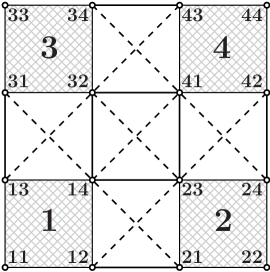
Figure 13: The $4\times 4$ superplaquette degree of freedom. Each spin carries two indices: a $2\times 2$ plaquette number and a coordinate within this plaquette.

Consistent with the previous work on the subject, we found the quantum paramagnetic phase in the interval $0.42\leq J_{2}/J_{1}\leq 0.66$. Main controversies revolve around the nature of this intermediate non-magnetic phase and of the quantum critical point separating it from the Néel – ordered state. We found that the paramagnetic phase is a plaquette crystal, preserving both lattice and spin rotational symmetries. Extrapolation of our numerical results to the thermodynamic limit suggests that the Ginzburg-Landau-Wilson paradigm of phase transitions is perfectly applicable in this case. Indeed, within the HMF, there is a group-subgroup relation between symmetries of the non-magnetic and Néel phases, which are thus separated by a second-order phase transition. On the contrary, such relation does not exist between the plaquette crystal and columnar antiferromagnetic phases, so the corresponding transition is of the first order. Our plaquette crystal is quite different from the usually proposed dimerized (bond-ordered) phases in this non-magnetic region.

We also proposed a way to include fluctuations around the HF ground state and showed that properties of the collective excitation spectrum are consistent with the overall picture of spontaneously broken symmetries. In particular, it was demonstrated that the quantum paramagnetic state is characterized by a finite gap in the excitation spectrum, which vanishes in the Néel and columnar phases, producing a doubly degenerate Goldstone mode.

Although currently there exists no known material whose ground state realizes the paramagnetic phase of the $J_{1}$-$J_{2}$ model, in the future momentum-resolved measurements, such as neutron diffraction methods, can be used to identify the plaquette crystal phase of the type proposed here. Its experimental signature will be the unbroken four-fold lattice rotational symmetry on both sides of the second-order phase transition at the critical point $J_{2}^{c1}$.

We acknowledge fruitful discussions with C. D. Batista, C. Esebbag and E. Fradkin. This work was supported in part by the Spanish MEC under grant No. FIS2006-12783-C03-01.

VII Appendix A: Superplaquette degree of freedom

Here we present details of the HF calculation which uses the $4\times 4$ superplaquette, shown in Fig. 13, as an elementary degree of freedom. It turns out that the full angular momentum basis is inconvenient, thus we use the $2\times 2$ plaquette product states in order to perform the mean-field calculations. Each spin is characterized by two indices: the plaquette number $i=1,\ldots,4$ and an index $n=1\ldots 4$, which specifies a vertex in the plaquette. The singlet sector of the superplaquette Hilbert space is spanned by the states:

$$|A\rangle=\sideset{}{{}^{\prime}}{\prod}_{i=1}^{4}|a_{i}\rangle,$$

where prime indicates the constraint $\sum_{i=1}^{4}M_{i}=0$. Using these states, we can write down matrix elements like

$$\langle a^{\prime}_{1}\ldots a^{\prime}_{4}|{\bm{S}}_{in}{\bm{S}}_{jn^{\prime}}|a_{1}\ldots a_{4}\rangle$$

in the compact form:

$$\langle A^{\prime}|{\bm{S}}_{in}{\bm{S}}_{jn^{\prime}}|A\rangle=\bigl{(}\sigma_{nn^{\prime}}\bigr{)}_{a_{i}a_{j}}^{a_{i}^{\prime}a_{j}^{\prime}}\prod_{l\neq i,j}\delta_{a_{l}^{\prime}a_{l}}$$ (17)

with the symmetric matrices $\bigl{(}\sigma_{nm}\bigr{)}_{a_{i}a_{j}}^{a_{i}^{\prime}a_{j}^{\prime}}=\bigl{(}\sigma_{mn}\bigr{)}_{a_{j}a_{i}}^{a_{j}^{\prime}a_{i}^{\prime}}=\bigl{(}\sigma_{nm}\bigr{)}^{a_{i}a_{j}}_{a_{i}^{\prime}a_{j}^{\prime}}$ defined as:

$$\bigl{(}\sigma_{nn^{\prime}}\bigr{)}_{a_{i}a_{j}}^{a_{i}^{\prime}a_{j}^{\prime}}= \sum_{K,M}\bigl{(}-1\bigr{)}^{L_{i}+L_{j}^{\prime}+K}\langle L_{i}^{\prime}M_{i}^{\prime}L_{j}^{\prime}M_{j}^{\prime}|L_{i}^{\prime}L_{j}^{\prime}KM\rangle\langle L_{i}M_{i}L_{j}M_{j}|L_{i}L_{j}KM\rangle\times$$

$$\qquad\qquad\times\left\{\begin{array}[]{ccc}L_{i}^{\prime}&L_{j}^{\prime}&K\\ L_{j}&L_{i}&1\end{array}\right\}\langle\lambda_{i}^{\prime}\|S_{n}\|\lambda_{i}\rangle\langle\lambda_{j}^{\prime}\|S_{n^{\prime}}\|\lambda_{j}\rangle,$$ (20)

The Hamiltonian of a single superplaquette consists of two parts: a diagonal one, involving only $2\times 2$ plaquette contributions and a non-diagonal part, which accounts for the plaquette interactions. The former is written down straightforwardly as a matrix:

$$\bigl{(}H_{\rm d}\bigr{)}_{A^{\prime}A}=\prod_{i}\delta_{a_{i}^{\prime}a_{i}}\sum_{i}\epsilon_{a_{i}},$$ (21)

where $\epsilon_{a}$ is the plaquette self-energy, Eq. (4). The non-diagonal part has the operator form:

$$H_{\rm nd} =J_{1}\bigl{[}({\bm{S}}_{14}+{\bm{S}}_{41})({\bm{S}}_{23}+{\bm{S}}_{32})+{\bm{S}}_{12}{\bm{S}}_{21}+{\bm{S}}_{13}{\bm{S}}_{31}+{\bm{S}}_{34}{\bm{S}}_{43}+{\bm{S}}_{24}{\bm{S}}_{42}\bigr{]}+$$

$$+J_{2}\bigl{[}{\bm{S}}_{12}{\bm{S}}_{23}+{\bm{S}}_{14}{\bm{S}}_{21}+{\bm{S}}_{23}{\bm{S}}_{42}+{\bm{S}}_{41}{\bm{S}}_{24}+{\bm{S}}_{34}{\bm{S}}_{41}+{\bm{S}}_{32}{\bm{S}}_{43}+$$ (22)

$$\quad\qquad+{\bm{S}}_{31}{\bm{S}}_{14}+{\bm{S}}_{13}{\bm{S}}_{32}+{\bm{S}}_{14}{\bm{S}}_{41}+{\bm{S}}_{32}{\bm{S}}_{23}\bigr{]}.$$

Let us now proceed with interaction terms in the $J_{1}$-$J_{2}$ Hamiltonian (1). Each superplaquette has 4 nearest and 4 next-nearest neighbors. Within each neighboring superplaquette we enumerate $2\times 2$ plaquettes by the indices 5, 6, 7, 8, so that $1\to 5$, $2\to 6$, $3\to 7$ and $4\to 8$. Enumeration of vertices within a plaquette stays the same. In this manner we have the symmetrized nearest neighbor

$$H_{1} =\frac{J_{1}}{4}\bigl{[}{\bm{S}}_{11}({\bm{S}}_{73}+{\bm{S}}_{62})+{\bm{S}}_{12}{\bm{S}}_{74}+{\bm{S}}_{13}{\bm{S}}_{64}+{\bm{S}}_{31}{\bm{S}}_{82}+{\bm{S}}_{34}{\bm{S}}_{52}+{\bm{S}}_{33}({\bm{S}}_{84}+{\bm{S}}_{51})+$$

$$\quad\qquad+{\bm{S}}_{21}{\bm{S}}_{83}+{\bm{S}}_{24}{\bm{S}}_{53}+{\bm{S}}_{22}({\bm{S}}_{84}+{\bm{S}}_{51})+{\bm{S}}_{43}{\bm{S}}_{61}+{\bm{S}}_{42}{\bm{S}}_{71}+{\bm{S}}_{44}({\bm{S}}_{73}+{\bm{S}}_{62})\bigr{]}+$$

$$+\frac{J_{2}}{4}\bigl{[}{\bm{S}}_{11}({\bm{S}}_{74}+{\bm{S}}_{64})+{\bm{S}}_{12}({\bm{S}}_{73}+{\bm{S}}_{83})+{\bm{S}}_{13}({\bm{S}}_{62}+{\bm{S}}_{82})+{\bm{S}}_{21}({\bm{S}}_{74}+{\bm{S}}_{84})$$ (23)

$$\quad\qquad+{\bm{S}}_{22}({\bm{S}}_{53}+{\bm{S}}_{83})+{\bm{S}}_{24}({\bm{S}}_{51}+{\bm{S}}_{71})+{\bm{S}}_{31}({\bm{S}}_{84}+{\bm{S}}_{64})+{\bm{S}}_{33}({\bm{S}}_{82}+{\bm{S}}_{52})+$$

$$\quad\qquad+{\bm{S}}_{34}({\bm{S}}_{51}+{\bm{S}}_{61})+{\bm{S}}_{42}({\bm{S}}_{73}+{\bm{S}}_{53})+{\bm{S}}_{43}({\bm{S}}_{62}+{\bm{S}}_{52})+{\bm{S}}_{44}({\bm{S}}_{71}+{\bm{S}}_{61})\bigr{]},$$

and next-nearest neighbor

$$H_{2}=\frac{J_{2}}{4}\bigl{[}{\bm{S}}_{11}{\bm{S}}_{84}+{\bm{S}}_{22}{\bm{S}}_{73}+{\bm{S}}_{33}{\bm{S}}_{62}+{\bm{S}}_{44}{\bm{S}}_{51}\bigr{]}$$ (24)

superplaquette interactions. Using Eq. (17), one can easily construct matrix elements of the operators (22)-(24), which are required to obtain the HF equation of the type (11).

Having computed the single-superplaquette ground state wavefunction $R^{0}_{A}=R^{0}_{a_{1}a_{2}a_{3}a_{4}}$, we can use it to determine the spin polarizations:

$$\langle{\rm HF}|S^{z}_{1n}|{\rm HF}\rangle=\bigl{(}S^{z}_{n}\bigr{)}_{a_{1}^{\prime}a_{1}}R {}^{0}_{a_{1}^{\prime}a_{2}a_{3}a_{4}}R^{0}_{a_{1}a_{2}a_{3}a_{4}};$$

$$\vdots$$

$$\langle{\rm HF}|S^{z}_{4n}|{\rm HF}\rangle=\bigl{(}S^{z}_{n}\bigr{)}_{a_{4}^{\prime}a_{4}}R {}^{0}_{a_{1}a_{2}a_{3}a_{4}^{\prime}}R^{0}_{a_{1}a_{2}a_{3}a_{4}},$$

where $\bigl{(}S^{z}_{n}\bigr{)}_{a^{\prime}a}$ is given by Eq. (13).

VIII Appendix B: Fluctuation corrections – superfluid mean-field

In this Appendix we extend the analysis of Sec. III by considering fluctuations around the HF ground state. While not unique, a natural way to achieve this goal is to perform a superfluid-type mean-field approximation. As a result one can obtain the collective spectrum and corrections to the GSE and magnetization. Of primary interest is, of course, the energy gap in the excitation spectrum.

The structure of the superfluid mean-field is similar to the Fetter-Bogoliubov approach to inhomogeneous Bose liquids Fetter_1972 . Although we shall present results only for the $2\times 2$ plaquette degree of freedom, it can equally be applied to the $4\times 4$ superplaquette case.

VIII.1 General formulation

Let us return to the original Hamiltonian (8) and explicitly separate out the condensate mode in the operators $\gamma_{ia}$:

$$\gamma_{ia}=g_{a}+\beta_{ia}.$$ (25)

The condensation will occur in a certain superposition of the single-plaquette states. The real-valued multiplet $g_{a}$ plays the role of a condensate wavefunction (CWF) Fetter_1972 . Here it is chosen to be spatially homogeneous, but inhomogeneous phases can also be included. The CWF is normalized to the condensate fraction:

$$\sum_{a}g_{a}^{2}=n_{0}.$$

The non-condensate bosonic operators $\beta_{ia}$ describe fluctuation corrections to the HF solution. If they are neglected, we naturally return to the results of Sec. III. It is important to observe, however, that the HF ground state corresponds to the Bose condensation on each lattice site, not only in the ${\bm{k}}=0$ mode.

The superfluid mean-field approximation amounts to enforcing the Schwinger boson constraint on average:

$$n_{0}+\frac{1}{N_{\Box}}\sum_{i,a}\langle\beta_{ia}^{\dagger}\beta_{ia}\rangle=1,$$ (26)

neglecting fluctuations in the condensate channel, and retaining only terms quadratic in $\beta$ in the Hamiltonian (8):

$$H =N_{\Box}\biggl{[}\frac{1}{2}\biggl{(}\mu n_{0}+\sum_{a}\epsilon_{a}g_{a}^{2}\biggr{)}-\mu n_{0}\biggr{]}+$$

$$+\sum_{i,a}(\epsilon_{a}-\mu)\beta_{ia}^{\dagger}\beta_{ia}+4\sum_{i,\sigma}\bigl{(}H_{\rm int}^{\sigma}\bigr{)}^{a_{1}^{\prime}a_{2}^{\prime}}_{a_{1}a_{2}}g_{a_{2}^{\prime}}g_{a_{2}}\beta_{ia_{1}^{\prime}}^{\dagger}\beta_{ia_{1}}+$$

$$+\sum_{\sigma,\langle ij\rangle_{\sigma}}\bigl{(}H_{\rm int}^{\sigma}\bigr{)}^{a_{1}^{\prime}a_{2}^{\prime}}_{a_{1}a_{2}}\bigl{[}g_{a_{1}^{\prime}}g_{a_{2}^{\prime}}(\beta_{ia_{1}}^{\dagger}\beta_{ja_{2}}^{\dagger}+\beta_{ia_{1}}\beta_{ja_{2}})+$$

$$\qquad\qquad\qquad\qquad+2g_{a_{1}}g_{a_{2}^{\prime}}\beta_{ia_{1}^{\prime}}^{\dagger}\beta_{ja_{2}}\bigr{]},$$ (27)

where we abbreviated $\langle ij\rangle_{\sigma}=\bigl{(}\langle ij\rangle,\langle\langle ij\rangle\rangle\bigr{)}$ and matrix elements of $H_{\rm int}^{\sigma}$ are given by Eq. (5).

Figure 14: Ground state energy for the self-consistent solution (main panel) and after the first iteration (inset). The critical point $J_{2}^{c1}$ becomes a $\lambda$-point. The absence of points in the main panel around $J_{2}^{c1}$ is due to bad convergence in the simulation.

The CWF $g_{a}$ is determined by the Gross-Pitaevskii equation, similar to the HF equation (11):

$$\biggl{\{}\epsilon_{a}\delta_{aa^{\prime}}+4\sum_{\sigma}\bigl{(}H_{\rm int}^{\sigma}\bigr{)}^{aa_{1}}_{a^{\prime}a_{2}}g_{a_{1}}g_{a_{2}}\biggr{\}}g_{a^{\prime}}=\mu g_{a},$$ (28)

which defines the chemical potential $\mu$ and guarantees the disappearance of linear terms in $\beta$ from the Hamiltonian of Eq. (27). It is clear that $g_{a}(n_{0}=1)=R_{a}^{0}$ and $\mu(n_{0}=1)=\varepsilon_{0}$. In other words, Eq. (28) reproduces the results of Sec. III, if $n_{0}$ is forced to be unity. Naturally, the first line in Eq. (27) coincides in this limit (up to the chemical potential) with the expression (12) for $E_{0}$. Quadratic terms in Eq. (27) represent fluctuation corrections to the HF results and constitute the focus of our analysis below.

Figure 15: Condensate fraction for the self-consistent solution (main panel) and after the first iteration (inset). Notice the shift of quantum phase transition points $J_{2}^{c1,2}$.

The next step is to transform the quadratic part ($H_{2}$) of the Hamiltonian in Eq. (27) into momentum space:

$$H_{2} =\sum_{{\bm{k}},a}(\epsilon_{a}-\mu)\beta_{{\bm{k}}a}^{\dagger}\beta_{{\bm{k}}a}+\sum_{{\bm{k}},\sigma}\bigl{(}H_{\rm int}^{\sigma}\bigr{)}^{a_{1}^{\prime}a_{2}^{\prime}}_{a_{1}a_{2}}\bigl{\{}\Theta_{\bm{k}}^{\sigma}\bigl{[}g_{a_{1}^{\prime}}g_{a_{2}^{\prime}}\times$$

$$\times(\beta_{{\bm{k}}a_{1}}^{\dagger}\beta_{-{\bm{k}}a_{2}}^{\dagger}+\beta_{{\bm{k}}a_{1}}\beta_{{\bm{k}}a_{2}})+2g_{a_{1}}g_{a_{2}^{\prime}}\beta_{{\bm{k}}a_{1}^{\prime}}^{\dagger}\beta_{{\bm{k}}a_{2}}\bigr{]}+$$

$$+4g_{a_{2}^{\prime}}g_{a_{2}}\beta_{{\bm{k}}a_{1}^{\prime}}^{\dagger}\beta_{{\bm{k}}a_{1}}\bigr{\}},$$ (29)

where $\Theta_{\bm{k}}^{\sigma}=(\cos k_{x}+\cos k_{y},2\cos k_{x}\cos k_{y})$ and ${\bm{k}}$ is defined within the plaquette Brillouin zone (i.e., there are $N_{\Box}$ ${\bm{k}}$- states). This Hamiltonian can be diagonalized by the Bogoliubov’s transformation:

$$\alpha_{{\bm{k}}\nu}= \sum_{a}\bigl{(}u_{{\bm{k}}a}^{\nu}\beta_{{\bm{k}}a}-v_{{\bm{k}}a}^{\nu}\beta_{-{\bm{k}}a}^{\dagger}\bigr{)};$$

$$\alpha_{-{\bm{k}}\nu}^{\dagger}= \sum_{a}\bigl{(}-v_{{\bm{k}}a}^{\nu}\beta_{{\bm{k}}a}+u_{{\bm{k}}a}^{\nu}\beta_{-{\bm{k}}a}^{\dagger}\bigr{)},$$ (30)

to a new set of bosonic operators $\alpha_{{\bm{k}}\nu}$, which represent quasiparticle excitations and annihilate the new ground state: $\alpha_{{\bm{k}}\nu}|\Psi_{0}\rangle=0$. Of course, only positive quasiparticle energies, labeled by $\nu$, have physical meaning, however, in order to obtain closure relations for the wavefunction $\bigl{(}u_{{\bm{k}}a}^{\nu},v_{{\bm{k}}a}^{\nu}\bigr{)}$ (which is, obviously, even in ${\bm{k}}$), we need to include zero-energy eigenvectors as well Ripka .

Figure 16: Self-consistently computed staggered magnetization, $M_{\rm stag}$, for $J_{2}\leq J_{2}^{c1}$ and columnar magnetization along the $x$-direction, $M_{\rm col}(x)$, for $J_{2}\geq J_{2}^{c2}$.

This completeness relation has the form, valid for all wavevectors:

$$\sum_{\nu}\bigl{(}u_{{\bm{k}}a}^{\nu}u_{{\bm{k}}b}^{\nu}-v_{{\bm{k}}a}^{\nu}v_{{\bm{k}}b}^{\nu}\bigr{)}= \delta_{ab};$$

$$\sum_{\nu}\bigl{(}u_{{\bm{k}}a}^{\nu}v_{{\bm{k}}b}^{\nu}-v_{{\bm{k}}a}^{\nu}u_{{\bm{k}}b}^{\nu}\bigr{)}= 0.$$ (31)

The amplitudes $u_{a}^{\nu}({\bm{k}})$ and $v_{a}^{\nu}({\bm{k}})$ are determined from Bogoliubov’s equations:

$$U_{ab}^{N}({\bm{k}})u_{{\bm{k}}b}^{\nu}+U_{ab}^{A}({\bm{k}})v_{{\bm{k}}b}^{\nu}= \omega_{\nu}({\bm{k}})u_{{\bm{k}}a}^{\nu};$$

$$U_{ab}^{A}({\bm{k}})u_{{\bm{k}}b}^{\nu}+U_{ab}^{N}({\bm{k}})v_{{\bm{k}}b}^{\nu}= -\omega_{\nu}({\bm{k}})v_{{\bm{k}}a}^{\nu},$$ (32)

where we have introduced symmetric matrices:

$$U_{ab}^{N}({\bm{k}})= \frac{1}{2}\bigl{(}\epsilon_{a}-\mu\bigr{)}\delta_{ab}+\sum_{\sigma}\bigl{(}H_{\rm int}^{\sigma}\bigr{)}^{aa_{1}}_{a_{2}b}\Theta_{\bm{k}}^{\sigma}g_{a_{1}}g_{a_{2}}+$$

$$\quad+2\sum_{\sigma}\bigl{(}H_{\rm int}^{\sigma}\bigr{)}^{aa_{1}}_{ba_{2}}g_{a_{1}}g_{a_{2}};$$ (33)

$$U_{ab}^{A}({\bm{k}})= \sum_{\sigma}\bigl{(}H_{\rm int}^{\sigma}\bigr{)}^{a_{1}a_{2}}_{ab}\Theta_{\bm{k}}^{\sigma}g_{a_{1}}g_{a_{2}}.$$

It follows from Eq. (32) that at each ${\bm{k}}$ the quasiparticle amplitudes obey the orthogonality conditions:

$$\sum_{a}\bigl{(}u_{{\bm{k}}a}^{\nu}u_{{\bm{k}}a}^{\nu^{\prime}}-v_{{\bm{k}}a}^{\nu}v_{{\bm{k}}a}^{\nu^{\prime}}\bigr{)}= \delta_{\nu\nu^{\prime}};$$

$$\sum_{a}\bigl{(}u_{{\bm{k}}a}^{\nu}v_{{\bm{k}}a}^{\nu^{\prime}}-v_{{\bm{k}}a}^{\nu}u_{{\bm{k}}a}^{\nu^{\prime}}\bigr{)}= 0.$$ (34)

For any value of ${\bm{k}}$ Bogoliubov’s equations (32) always have at least two zero eigenvalues, which correspond to the zero-norm eigenvector $u=-v=g$. This means that our case differs fundamentally from the canonical superfluid Bose gas: instead of having a macroscopic number of particle in one particular energy state, we obtain a macroscopic number (equal to $N_{\Box}$) of condensation modes, each containing less than one boson.

The quasiparticle energy equals $2\omega_{\nu}({\bm{k}})$ and the GSE, condensate fraction and spin polarization are expressed in terms of $u_{{\bm{k}}a}^{\nu}$ and $v_{{\bm{k}}a}^{\nu}$ as:

$$\frac{E_{0}}{N}= \frac{1}{8}\biggl{(}\mu n_{0}+\sum_{a}\epsilon_{a}g_{a}^{2}\biggr{)}+\frac{1}{4}\mu(1-n_{0})-$$

$$\quad-\frac{2}{N}\sideset{}{{}^{\prime}}{\sum}_{{\bm{k}},\nu,a}\omega_{\nu}({\bm{k}})\bigl{(}v_{{\bm{k}}a}^{\nu}\bigr{)}^{2};$$ (35)

$$n_{0}= 1-\frac{1}{N_{\Box}}\sideset{}{{}^{\prime}}{\sum}_{{\bm{k}},\nu,a}\bigl{(}v_{{\bm{k}}a}^{\nu}\bigr{)}^{2};$$

$$\langle S^{z}_{in}\rangle= \bigl{(}S^{z}_{n}\bigr{)}_{a^{\prime}a}\biggl{[}g_{a^{\prime}}g_{a}+\frac{1}{N_{\Box}}\sideset{}{{}^{\prime}}{\sum}_{{\bm{k}},\nu}v^{\nu}_{{\bm{k}}a^{\prime}}v^{\nu}_{{\bm{k}}a}\biggr{]}.$$

In this expression ${\bm{k}}$-summations are extended over the plaquette Brillouin zone and $\nu$-summations over positive eigenvalues of Eq. (32), as indicated by the primes.

Figure 17: The lowest excitation branch $\omega_{1}({\bm{k}})$ along the $[10]$ and $[11]$ directions for three values of $J_{2}/J_{1}$ chosen in different phases.

VIII.2 Results for the symmetric plaquette covering

The condensate fraction $n_{0}$ should, in principle, be determined self-consistently. The approximation is reasonable if $n_{0}\sim 1$. However, close to the phase transition points this is not true, since fluctuations are very large in their vicinity. But deeply in each phase the approximation works reasonably well, because $n_{0}$ turns out to be of the order of $0.9$. Results of the numerical solution of Eqs. (28), (32) and (35) for the symmetric covering of the lattice with $2\times 2$ plaquettes are shown in Figs. 14-17. The system size is $100\times 100$ plaquettes and periodic boundary conditions are assumed. Figures’ main panels correspond to the self-consistent solution and their insets give results after the first iteration, which is equivalent to solving the time-dependent Gross-Pitaevskii equation Ripka . Due to bad convergence close to the transition points (see, for instance, Fig. 14) the values of $J_{2}^{c1}$ and $J_{2}^{c2}$ were determined by extrapolation: $J_{2}^{c1}\approx 0.33J_{1}$ and $J_{2}^{c2}\approx 0.65J_{1}$. The large shift of $J_{2}^{c1}$ compared to the HF value is due to fluctuations in the $\beta$-channel, which renders this point to be a $\lambda$-point, reduces the nominal value of the magnetization in the Néel phase down to $M(J_{2}=0)\approx 0.37$ (Fig. 16), and causes a great suppression of the condensate, as shown in Fig. 15.

However, the most interesting quantity to observe is the gap in the excitation spectrum. Due to the homogeneity of the plaquette lattice, it occurs at ${\bm{k}}=0$ and is shown in Fig. 11.

Technically, one may show that its very existence reflects the nature of the ground state in the paramagnetic phase. Indeed, introducing linear combinations of the amplitudes $u$ and $v$: $\varphi=u+v$ and $\chi=u-v$, Bogoliubov’s Eq. (32) can be rewritten in the form:

$$\bigl{(}U^{N}+U^{A}\bigr{)}\bigl{(}U^{N}-U^{A}\bigr{)}\chi=\omega^{2}\chi.$$

In the non-magnetic phase the condensation occurs in the lowest plaquette state $|1100\rangle$: $g_{a}=\sqrt{n_{0}}\delta_{a,1100}$ and the chemical potential coincides with its energy: $\mu=\epsilon_{1100}$. Moreover, the matrix $\sum_{\sigma}\bigl{(}H_{\rm int}^{\sigma}\bigr{)}_{b,1100}^{a,1100}$ vanishes. Writing down the remaining matrices in (33) at ${\bm{k}}=0$, it is easy to see that there exists only one vector $\chi$, which is annihilated by $\bigl{(}U^{N}-U^{A}\bigr{)}$. Outside the intermediate region this simple situation is not valid and there exist three eigenvectors $\chi$, which correspond to $\omega^{2}=0$. One of them is the condensate mode and should be discarded. The other two give doubly degenerate Goldstone modes in the Néel and columnar phases. Here the self-consistent field, determined by $g_{a}$, breakes the spin-rotational symmetry of the original Hamiltonian. However, since the CWF $g_{a}$ belongs to the $M=0$ subspace, the generator $S_{z}$ remains an integral of motion. Thus, there should be two Goldstone modes associated with rotations around the $x$ and $y$ axes Ripka .

Our approximation correctly describes the excitation spectrum only at small ${\bm{k}}$. However, this is more than enough to observe that the collective modes are of the spin-wave type in the Néel and columnar phases, while in the paramagnetic phase the excitation band is parabolic. These conclusions are summarized in Fig. 17, where we show the lowest branch $\omega_{1}({\bm{k}})$ along two directions ${\bm{k}}\|[10]$ and ${\bm{k}}\|[11]$ for three values of $J_{2}/J_{1}$, chosen in different phases.

References

- (1) P. Carretta, R. Melzi, N. Papinutto and P. Millet, Phys. Rev. Lett. 88, 047601 (2002); A. Bombardi, J. Rodriguez-Carvajal, S. Di Matteo, F. de Bergevin, L. Paolasini, P. Carretta, P. Millet and R. Caciuffo, ibid. 93, 027202 (2004).
- (2) P. Carretta, N. Papinutto, C. B. Azzoni, M. C. Mozzati, E. Pavarini, S. Gonthier and P. Millet, Phys. Rev. B66, 094420 (2002).
- (3) R. Nath, A. A. Tsirlin, H. Rosner and C. Geibel, arXiv:0803.3535v1 [cond-mat.str-el].
- (4) S. Sachdev, Quantum Phase Transitions (Cambridge University Press, Cambridge, 1999).
- (5) G. Misguich and C. Lhuillier in Frustrated Spin Systems, edited by H. T. Diep (World Scientific, Singapore, 2004).
- (6) L. Capriotti and S. Sorella, Phys. Rev. Lett. 84, 3173 (2000).
- (7) L. Capriotti, F. Becca, A. Parola and S. Sorella, Phys. Rev. Lett. 87, 097201 (2001).
- (8) M. S. L. du Croo de Jongh, J. M. J. van Leeuwen and W. van Saarloos, Phys. Rev. B62, 14844 (2000).
- (9) R. Darradi, O. Derzhko, R. Zinke, J. Schulenburg, S. E. Krueger and J. Richter, Phys. Rev. B78, 214415 (2008).
- (10) R. R. P. Singh, Z. Weihong, C. J. Hamer and J. Oitmaa, Phys. Rev. B60, 7278 (1999).
- (11) K. Takano, Y. Kito, Y. Ono and K. Sano, Phys. Rev. Lett. 91, 197202 (2003).
- (12) V. Kotov, J. Oitmaa, O. Sushkov and Z. Weihong, Phys. Rev. B60, 14613 (1999).
- (13) V. Lante and A. Parola, Phys. Rev. B73, 094427 (2006).
- (14) N. Read and S. Sachdev, Phys. Rev. Lett. 66, 1773 (1991).
- (15) T. Senthil, L. Balents, S. Sachdev, A. Vishwanath and M. P. A. Fisher, Phys. Rev. B70, 144407 (2004).
- (16) L. D. Landau, E. M. Lifshitz and L. P. Pitaevskii, Statistical Physics, parts. 1 and 2 (Butterworth-Heinemann, New-York, 1999); K. G. Wilson and J. Kogut, Phys. Rep. 12, 75 (1974).
- (17) E. Manousakis, Rev. Mod. Phys. 63, 1 (1991).
-
(18)
That the translational symmetry is broken in the Néel phase is easy
to see, if one assumes broken spin symmetry. Then, due
to the principle of weakening of correlations, the staggered
correlation function satisfies:
which can be constant only if depends on . - (19) J. Sirker, Z. Weihong, O. Sushkov and J. Oitmaa, Phys. Rev. B73, 184420 (2006).
- (20) A. W. Sandvik, Phys. Rev. Lett. 98, 227202 (2007).
- (21) C. D. Batista and S. A. Trugman, Phys. Rev. Lett. 93, 217202 (2004).
- (22) G. Ortiz and C. D. Batista, Phys. Rev. B67, 134301 (2003); in Condensed Matter Theories, vol. 18, M. de Llano et al. (ed.), Nova Science Publishers, 2003.
- (23) M. van den Bossche, F.-C. Zhang and F. Mila, Eur. Phys. J. B17, 367 (2000).
- (24) E. Altman and A. Auerbach, Phys. Rev. B65, 104508 (2002).
- (25) A. R. Edmonds, Angular Momentum in Quantum Mechanics (Princeton University Press, Princeton, 1957).
- (26) A. Auerbach, Interacting Electrons and Quantum Magnetism (Springer-Verlag, New York, 1994).
- (27) N. Trivedi and D. M. Ceperley, Phys. Rev. B40, 2737 (1989).
- (28) A. L. Fetter, Ann. Phys. 70, 67 (1972).
- (29) C. K. Majumdar and D. K. Ghosh, J. Math. Phys. 10, 1388 (1969).
- (30) K. Okamoto and K. Nomura, Phys. Lett. A169, 433 (1992).
- (31) E. H. Lieb, T. D. Schultz and D. C. Mattis, Ann. Phys. 16, 407 (1961).
- (32) M. B. Hastings, Phys. Rev. B69, 104431 (2004).
- (33) M. E. Fisher, Phys. Rev. 124, 1664 (1961).
- (34) F. Kruger and S. Scheidl, Europhys. Lett. 74, 896 (2006).
- (35) S. R. White, Phys. Rev. Lett. 77, 3633 (1996).
- (36) J. P. Blaizot and G. Ripka, Quantum theory of finite systems (The MIT Press, Cambridge, 1986).