Chimera states in heterogeneous networks

Abstract

Chimera states in networks of coupled oscillators occur when some fraction of the oscillators synchronise with one another, while the remaining oscillators are incoherent. Several groups have studied chimerae in networks of identical oscillators, but here we study these states in heterogeneous models for which the natural frequencies of the oscillators are chosen from a distribution. For a model consisting of two subnetworks we obtain exact results by reduction to a finite set of differential equations, and for a network of oscillators in a ring we generalise known results. We find that heterogeneity can destroy chimerae, destroy all states except chimerae, or destabilise chimerae in Hopf bifurcations, depending on the form of the heterogeneity.

Synchronisation of interacting oscillators is a problem of fundamental importance, with applications from Josephson junction circuits to neuroscience [19, 24, 22, 27]. Since oscillators are unlikely to be identical, the effects of heterogeneity on their collective behaviour is of interest. One well-studied system of heterogeneous phase oscillators is the Kuramoto model [4, 9, 23], for which there is global coupling. Generalisations of this model with nonlocal coupling [3, 21, 2, 10, 16], or several populations of oscillators [1], have shown interesting types of behaviour referred to as “chimera” states in which some oscillators are synchronised with one another while the remainder are incoherent. Even though the effects of heterogeneity on synchronisation have been emphasised in the past [4, 13, 9, 23], all chimerae have so far been studied in networks of identical oscillators. This raises the obvious question: do chimerae exist in networks of nonidentical oscillators? Here we address the question analytically, first using recent results to exactly derive a finite set of differential equations governing the dynamics of chimerae in two coupled networks of heterogeneous phase oscillators, and then using a similar idea to extend the results of Abrams and Strogatz [3] for chimera states in a ring of coupled oscillators.

1 Introduction

Networks of coupled oscillators have been studied for many years [24, 13, 1, 3, 19, 20, 5]. One well-known system is the Kuramoto model [4, 9, 6, 10, 23] of phase oscillators. In the last few years several authors have studied “chimera” states in networks of identical Kuramoto oscillators, in which some oscillators are synchronised with one another while the remainder are incoherent. Much analytical progress has been made in the study of these states [1, 3, 21, 2, 10, 16]. It is very unlikely that any physical system being modelled by a network of coupled oscillators will have identical units, so the robustness of chimerae to network heterogeneity is naturally of interest. Certain networks of coupled oscillators are known to have non-generic properties [25, 26], and it is of interest to know whether chimera states are generic and stable (and thus expected to be generally observed) or not.

Here we conduct an analytical investigation into the robustness of previously-studied chimerae with respect to heterogeneity in the intrinsic frequencies of oscillators. We find that chimerae are robust with respect to this type of heterogeneity, and show some of the bifurcations that chimera and other states undergo as the oscillators in the network are made more dissimilar. Our results provide more evidence that the Ott-Antonsen ansatz [17] correctly describes attracting states in Kuramoto-type networks when the oscillators are not identical. Some of the ideas here have recently been used by others to study a single population of oscillators with a bimodal frequency distribution [14] and the periodically forced Kuramoto model [7].

Note that the term “chimera” has been used in the past to refer to certain states in networks of identical oscillators [16, 21, 1, 3], but here we also use the term to describe similar states in heterogeneous networks in the obvious way. A state found by numerically continuing from a chimera state in a network of identical oscillators is also referred to as a chimera.

In Sec. 2 we present the first model of two coupled networks, then consider its continuum limit and use the remarkable recent result of Ott and Antonsen [17] to derive three ODEs which exactly describe some of its behaviour. In Sec. 3 we perform a limited bifurcation analysis of these ODEs and interpret the results. In Secs. 4 and 5 we consider other distributions of the intrinsic oscillator frequencies, and generalisations, respectively. In Sec. 6 we consider oscillators on a ring.

2 Two coupled networks

We first consider two networks of coupled oscillators with uniform coupling between oscillators within each network, and a weaker coupling to those in the other network. Our model equations are

$$\frac{d\theta_{i}^{k}}{dt}=\omega_{i}^{k}+\sum_{m=1}^{2}\frac{K_{km}}{N}\sum_{j=1}^{N}\sin{(\theta_{j}^{m}-\theta_{i}^{k}-\alpha)}$$ (1)

for $i=1,\ldots N$ and $k=1,2$, where the natural frequencies $\omega_{i}^{k}$ are chosen from a distribution $g_{k}(\omega^{k})$. Our system is the same as that of Montbrió et al. [15]; the system of Abrams et al. [1] is a special case of that studied here. A similar system was studied by Barreto et al. [6], but their focus was the onset of synchrony, as was Montbrió et al’s. Like Abrams et al. [1], we choose $K_{11}=K_{22}=\mu$ and $K_{12}=K_{21}=\nu$, set $\mu+\nu=1$ (by rescaling time if necessary), and choose $\mu>\nu$. We define $A=\mu-\nu$ and $\beta=\pi/2-\alpha$. Abrams et al. found that for $\beta$ and $A$ sufficiently small and positive (and all $\omega_{i}^{k}$ equal), both the completely synchronised state ($\theta_{j}^{m}=\theta_{i}^{k}$ for all $j,i,m,k$) and the chimera state (all oscillators in one population perfectly synchronised, all oscillators in the other population incoherent) were stable.

We take the continuum limit of (1), letting $N\rightarrow\infty$. The system is then described by the probability density function (PDF) $f_{k}(\omega^{k},\theta^{k},t)$ for each population $k$. We define two order parameters

$$z_{k}(t)=\int_{-\infty}^{\infty}\int_{0}^{2\pi}\exp{(i\theta^{k})}f_{k}(\omega^{k},\theta^{k},t)\ d\theta^{k}\ d\omega^{k}$$ (2)

for $k=1,2$. Each $f_{k}$ satisfies a continuity equation

$$\frac{\partial f_{k}}{\partial t}+\frac{\partial}{\partial\theta^{k}}(f_{k}v_{k})=0$$ (3)

where the velocity

$$v_{k} = \omega^{k}+\{\exp{[-i(\theta^{k}+\alpha)]}(\mu z_{k}+\nu z_{k^{\prime}})$$ (4)

$$-\exp{[i(\theta^{k}+\alpha)]}(\mu\bar{z}_{k}+\nu\bar{z}_{k^{\prime}})\}/(2i),$$

$k^{\prime}=3-k$, and an overbar denotes the complex conjugate. Writing $f_{k}$ as a Fourier series in $\theta^{k}$ we have

$$f_{k}(\omega^{k},\theta^{k},t)=\frac{g_{k}(\omega^{k})}{2\pi}\left[1+\left\{\sum_{n=1}^{\infty}h_{n}(\omega^{k},t)\exp{(in\theta^{k})}+c.c.\right\}\right]$$ (5)

where “$c.c.$” denotes the complex conjugate of the previous term. Substituting (5) into (3) and (2), one can derive an infinite set of integro-differential equations for the $h_{n}$ [15]. However, Ott and Antonsen [17] noticed that for the special choice

$$h_{n}(\omega^{k},t)=\left[a_{k}(\omega^{k},t)\right]^{n}$$ (6)

i.e. $h_{n}$ is $a_{k}$ raised to the $n$th power, all of these differential equations are actually the same, and we are left with a single PDE governing the dynamics of $a_{k}(\omega^{k},t)$:

$$\frac{\partial a_{k}}{\partial t}+i\omega^{k}a_{k}-(e^{i\alpha}/2)(\mu\bar{z}_{k}+\nu\bar{z}_{k^{\prime}})$$

$$+(e^{-i\alpha}/2)(\mu z_{k}+\nu z_{k^{\prime}})a_{k}^{2} = 0$$ (7)

where

$$z_{k}(t)=\int_{-\infty}^{\infty}\bar{a}_{k}(\omega^{k},t)g_{k}(\omega^{k})\ d\omega^{k}$$ (8)

The ansatz (6) is not trivial, and the reduction from an infinite set of differential equations to one is remarkable. Ott and Antonsen [17] give more detail on the circumstances under which this ansatz is valid, and we discuss its usefulness in describing attracting states below.

As is well-known [15, 17, 9, 14], if $g_{k}$ is a Lorentzian distribution the integral (8) can be evaluated analytically. Suppose that

$$g_{k}(\omega^{k}) = \frac{D_{k}/\pi}{(\omega^{k}-\Omega_{k})^{2}+D_{k}^{2}}$$ (9)

i.e. the $\omega^{k}_{i}$ are from a distribution centred at $\Omega_{k}$ with half-width-at-half-maximum $D_{k}$. Then $z_{k}(t)=\bar{a}_{k}(\Omega_{k}-iD_{k},t)$ and evaluating (7) at $\omega^{k}=\Omega_{k}-iD_{k}$ we obtain

$$\frac{d\bar{z}_{k}}{\partial t}+(D_{k}+i\Omega_{k})\bar{z}_{k}-(e^{i\alpha}/2)(\mu\bar{z}_{k}+\nu\bar{z}_{k^{\prime}})$$

$$+(e^{-i\alpha}/2)(\mu z_{k}+\nu z_{k^{\prime}})\bar{z}_{k}^{2} = 0$$ (10)

i.e. a complex ODE for each $k$. Writing $z_{1}=r_{1}e^{-i\phi_{1}}$ and $z_{2}=r_{2}e^{-i\phi_{2}}$ and defining $\phi=\phi_{1}-\phi_{2}$ we obtain the three real ODEs:

$$\frac{dr_{1}}{dt} = -D_{1}r_{1}+\left(\frac{1-r_{1}^{2}}{2}\right)[\mu r_{1}\cos{\alpha}+\nu r_{2}\cos{(\phi-\alpha)}]$$ (11)

$$\frac{dr_{2}}{dt} = -D_{2}r_{2}+\left(\frac{1-r_{2}^{2}}{2}\right)[\mu r_{2}\cos{\alpha}+\nu r_{1}\cos{(\phi+\alpha)}]$$ (12)

$$\frac{d\phi}{dt} = \left(\frac{r_{1}^{2}+1}{2r_{1}}\right)[\mu r_{1}\sin{\alpha}-\nu r_{2}\sin{(\phi-\alpha)}]+\Omega_{2}$$ (13)

$$- \left(\frac{r_{2}^{2}+1}{2r_{2}}\right)[\mu r_{2}\sin{\alpha}+\nu r_{1}\sin{(\phi+\alpha)}]$$

where, without loss of generality, we have set $\Omega_{1}=0$. When $D_{1}=D_{2}=\Omega_{2}=0$, we recover the results of Abrams et al. [1]. In particular, $r_{1}=1$ ($\theta^{1}_{i}$ all equal) is invariant. If $r_{1}=1$, there also exists the perfect synchrony state ($r_{2}=1,\phi=0$) and, depending on parameters (see Fig. 4 in [1]) two other fixed points with $r_{2}\neq 1$ (the chimerae). When they exist, one of these fixed points is a saddle while the other is either stable or unstable, changing stability via a supercritical Hopf bifurcation. We now proceed with a limited analysis of (11)-(13).

3 Results

3.1 Varying distribution widths, no frequency offset

First consider the case when $D_{1}=D_{2}=D$ and $\Omega_{2}=0$. The system (11)-(13) possesses $\mathbb{Z}_{2}$ symmetry: $(r_{1},r_{2},\phi)\rightarrow(r_{2},r_{1},-\phi)$. We choose $A=0.2$ and $\beta=0.07$ so that for $D=0$, there exist five fixed points of (11)-(13): the perfect synchrony state $(r_{1},r_{2},\phi)=(1,1,0)$ and two chimerae (one stable and one a saddle) for which $r_{1}=1$ and $r_{2}\neq 1$ and $\phi\neq 0$, and their symmetrically related states. The fixed points of (11)-(13) and their stability as a function of $D$ are shown in Fig. 1.

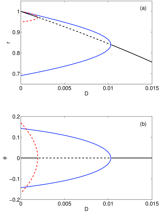
Figure 1: (Colour online) Fixed points of (11)-(13) when $D_{1}=D_{2}=D,\Omega_{2}=0$. (a): $r_{1}$ and $r_{2}$ as a function of $D$. (b): $\phi$ as a function of $D$. Blue curve: stable chimera. Red curve: saddle chimera. Black curve: symmetric state ($r_{1}=r_{2}$). Solid lines indicate stable solutions, dashed lines unstable. Other parameters: $A=0.2,\beta=0.07$.

There are several interesting observations to be made here. Firstly (for these parameter values), increasing the heterogeneity of the network first destabilises the symmetric state ($r_{1}=r_{2}$), then restabilises it. Secondly, increasing the heterogeneity actually decreases the width of the angular distribution of the unsynchronised population in the chimera state (lower blue branch in panel (a) of Fig. 1).

3.2 Varying one distribution width, no frequency offset

Now consider varying $D_{2}$, while $D_{1}=\Omega_{2}=0$. The system no longer possesses any symmetry, so the effect of increasing $D_{2}$ from zero on the chimerae with $r_{1}=1,r_{2}\neq 1$ will be different from its effect on the chimerae with $r_{1}\neq 0,r_{2}=1$. We choose $A=0.2$ and $\beta=0.1$, so that as before, when $D_{2}=0$ there exist five fixed points of (11)-(13). Results are shown in Fig. 2. With five solutions to track, we do not show $\phi$. Also, even though $D_{2}<0$ is not physically meaningful we plot fixed points for $D_{2}<0$ to show how branches of solutions are connected.

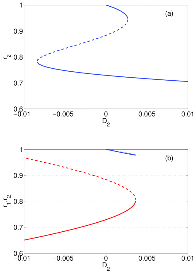
Figure 2: (Colour online) Fixed points of (11)-(13) when $D_{1}=\Omega_{2}=0$. (a): $r_{2}$ as a function of $D_{2}$ when $r_{1}=1$. (b): $r_{1}$ (red) and $r_{2}$ (blue) as a function of $D_{2}$. Solid lines indicate stable solutions, dashed lines unstable. Other parameters: $A=0.2,\beta=0.1$.

Panel (a) in Fig. 2 shows fixed points for which $r_{1}=1$ (recall that we are making population 2 heterogeneous). As $D_{2}$ is increased, the perfectly synchronous solution that exists at $D_{2}=0$ is destroyed in a saddle-node bifurcation, while the chimera with population 2 desynchronised persists. Panel (b) shows the fate of the two chimerae (one stable and one a saddle) for which $r_{2}=1$ when $D_{2}=0$. We see that they are both destroyed in a saddle-node bifurcation as $D_{2}$ is increased. From this figure we see that if one population is made sufficiently heterogeneous, the only solution that persists is the chimera for which the oscillators in that population are desynchronised. Interestingly, if $D_{2}$ is increased to larger values ($D_{2}\approx 0.1$), the state where both populations are in the “splay” state, with uniform angular density, i.e. $r_{1}=r_{2}=0$ and $\phi$ is no longer meaningful, becomes stable (not shown).

3.3 Varying frequency offset $\Omega_{2}$

We now consider varying $\Omega_{2}$ with $D_{1}=D_{2}=0$. Since we are interested in states for which at least one of the populations is in complete synchrony we set $r_{1}=1$ and only consider (12)-(13). The completely synchronised state, $(r_{2},\phi)=(1,0)$, exists when $\Omega_{2}=0$, and as $\Omega_{2}$ is increased it persists as the fixed point $(r_{2},\phi)=(1,\phi)$, where $\phi$ is the solution closest to zero of $2\nu\cos{\alpha}\sin{\phi}=\Omega_{2}$. Numerical results are shown in Fig. 3.

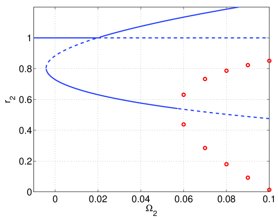
Figure 3: (Colour online) $r_{2}$ as a function of $\Omega_{2}$, when $r_{1}=1$. Solid lines indicate stable fixed points of (11)-(13), dashed lines unstable. Circles are the maximum and minimum of $r_{2}$ during stable periodic oscillations. Note that the branch with $r_{2}>1$ is not physically meaningful. Other parameters: $A=0.2,\beta=0.1$.

We see that as $\Omega_{2}$ is increased from zero, the synchronised state for which $r_{2}=1$ is destroyed in a transcritical bifurcation involving the saddle chimera, while the stable chimera undergoes a supercritical Hopf bifurcation, leading to oscillations in $r_{2}$ and $\phi$. However, decreasing $\Omega_{2}$ from zero causes destruction of the stable chimera in a saddle-node bifurcation with the saddle chimera. For these parameter values, one can see that the stable chimera is much more robust to speeding up the asynchronous oscillators, as opposed to a slowing them down.

3.4 Discussion

Our bifurcation analysis in this section has found all four codimension-1 bifurcations of ODEs (saddle-node, pitchfork, transcritical and Hopf) and a two-parameter study is likely to find higher codimension bifurcations.

Pikovsky and Rosenblum [18] recently studied (1) with identical $\omega_{i}^{k}$ (i.e. the system of Abrams et al. [1], and our system when $D_{1}=D_{2}=\Omega_{2}=0$) as a special case and found that the ansatz (6) did not completely describe the possible dynamics of this system. However, Pikovsky and Rosenblum [18] and other authors [14] found that when the oscillators are non-identical, this ansatz does successfully allow one to describe attracting states. We also find this behaviour here: extensive numerical simulations show that the stable states shown in Figs. 1 and 2 for $D,D_{2}>0$ are attracting, and that the angular distributions of these stable states are given by (5)-(6), even if the initial distributions are not. However, the same cannot be said for the results in Fig. 3, for which oscillators within each of the two networks are identical. This figure correctly predicts the dynamics if the initial angular distribution is given by (5)-(6) but other initial conditions give solutions not described by Fig. 3 (not shown). This relationship between initial conditions and dynamics when oscillators within each network are identical was also noticed by Montbrió et al. [15]. The results in Fig. 3 are likely to be a subset of those that could be found using the approach in Ref. [18].

In related results, Montbrió et al. [15] fixed $\Omega_{2}\neq 0$ and varied both $\alpha$ and $\nu$ and found chimera states, both for homogeneous and heterogeneous networks.

4 Other distributions

Now we consider the effects of choosing the $\omega^{k}_{i}$ from distributions other than the Lorentzian, first numerically and then analytically.

4.1 Gaussian distribution: numerical simulations

Figure 4 shows the results of fitting the time-dependent PDF

$$f_{k}(\theta,t) = \frac{1}{2\pi}\left[1+\left\{\sum_{n=1}^{\infty}\left(r_{k}e^{i\phi_{k}}\right)^{n}e^{in\theta}+c.c.\right\}\right]$$ (14)

$$= \frac{1-r_{k}^{2}}{2\pi[1-2r_{k}\cos{(\phi_{k}-\theta)}+r_{k}^{2}]}$$

to each population in simulations of (1) after transients, where all $\omega_{i}^{k}$ are chosen from a normal distribution of mean zero and standard deviation $\sigma$. We found that both $r_{1}$ and $r_{2}$ tended to constant values, as did $\phi_{2}-\phi_{1}$ (not shown). Only stable states are shown in Fig. 4, but the results are compatible with those shown in Fig. 1, suggesting that there is nothing special about the Lorentzian distribution, as has been noted by others [14, 7]. The unstable states could presumably be found using the “equation-free” method [13, 8, 12] of analysing low-dimensional descriptions of high-dimensional systems, under the assumption that these states are also exactly described by the variables $r,\phi$ for each population.

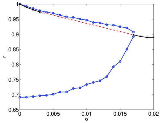
Figure 4: (Colour online) $r_{1}$ and $r_{2}$ fitted to simulations of (1), where all $\omega_{i}^{k}$ are chosen from a normal distribution of mean zero and standard deviation $\sigma$. Blue circles joined by a line: stable chimera. Black crosses joined by a line: stable symmetric state ($r_{1}=r_{2}$). Red dashed line: presumed unstable symmetric state. Compare with Fig. 1. See the text for details on the fitting. Other parameters: $A=0.2,\beta=0.07,N=1000$.

4.2 Another distribution

As an alternative [17], we suppose that the $\omega_{i}^{k}$ are chosen from the distribution

$$g_{k}(\omega)=\frac{\sqrt{2}s_{k}^{3}}{\pi}\left(\frac{1}{\omega^{4}+s_{k}^{4}}\right)$$ (15)

which has mean zero (for simplicity) and variance $s_{k}^{2}$. This $g_{k}(\omega)$ has poles at $\omega=s_{k}(\pm 1\pm i)/\sqrt{2}$, and the integral (8) gives

$$z_{k}=\left(\frac{1+i}{2}\right)z_{k}^{-}+\left(\frac{1-i}{2}\right)z_{k}^{+}$$ (16)

where $z_{k}^{\pm}$ satisfy

$$\frac{dz^{\pm}_{k}}{dt}-\left[s_{k}(1\pm i)/\sqrt{2}\right]z^{\pm}_{k}-(e^{-i\alpha}/2)(\mu z_{k}+\nu z_{k^{\prime}})$$

$$+(e^{i\alpha}/2)(\mu\bar{z}_{k}+\nu\bar{z}_{k^{\prime}})\left(z^{\pm}_{k}\right)^{2}=0$$ (17)

Thus we have four coupled complex ODEs, rather than the two (10). This can clearly be generalised to other distributions which are rational functions of $\omega$.

5 Generalisations

We now briefly mention several generalisations of the results above. Suppose that the system (1) is periodically forced, i.e. we add the term $\Lambda_{k}\sin{(\widehat{\Omega}t-\theta_{i}^{k})}$ to (1), as done recently for a single population [7]. Going to a coordinate frame rotating with angular frequency $\widehat{\Omega}$, we find that (10) is replaced by

$$\frac{d\bar{z}_{k}}{\partial t}+(D_{k}+i(\Omega_{k}-\widehat{\Omega}))\bar{z}_{k}-\left[\frac{\Lambda_{k}+e^{i\alpha}(\mu\bar{z}_{k}+\nu\bar{z}_{k^{\prime}})}{2}\right]$$

$$+\left[\frac{\Lambda_{k}+e^{-i\alpha}(\mu z_{k}+\nu z_{k^{\prime}})}{2}\right]\bar{z}_{k}^{2}=0$$

The system is no longer invariant under a translation of time, so during the derivation of ODEs like (11)-(13) we find that we need both $\phi_{1}$ and $\phi_{2}$, not just their difference.

Another possibility is that there is a uniform delay of $\tau$ between the two populations, but zero delay within them, i.e. we replace $\theta_{j}^{m}$ in (1) by $\theta_{j}^{m}(t-\tau)$ when $m=k^{\prime}$. The effect of this is to replace $z_{k^{\prime}}(t)$ in (10) by $z_{k^{\prime}}(t-\tau)$ and the equivalent of (11)-(13) is now the four delay differential equations:

$$\frac{dr_{1}}{dt}+D_{1}r_{1}+\left(\frac{r_{1}^{2}-1}{2}\right)[\mu r_{1}\cos{\alpha}+\nu r_{2}(t-\tau)\cos{\{\phi_{1}-\phi_{2}(t-\tau)-\alpha\}}] = 0$$

$$\frac{d\phi_{1}}{dt}-\left(\frac{r_{1}^{2}+1}{2r_{1}}\right)[\mu r_{1}\sin{\alpha}-\nu r_{2}(t-\tau)\sin{\{\phi_{1}-\phi_{2}(t-\tau)-\alpha\}}] = 0$$

$$\frac{dr_{2}}{dt}+D_{2}r_{2}+\left(\frac{r_{2}^{2}-1}{2}\right)[\mu r_{2}\cos{\alpha}+\nu r_{1}(t-\tau)\cos{\{\phi_{2}-\phi_{1}(t-\tau)-\alpha\}}] = 0$$

$$\frac{d\phi_{2}}{dt}+\Omega_{0}-\left(\frac{r_{2}^{2}+1}{2r_{2}}\right)[\mu r_{2}\sin{\alpha}-\nu r_{1}(t-\tau)\sin{\{\phi_{2}-\phi_{1}(t-\tau)-\alpha\}}] = 0$$

If all of the variables on the RHS of (1) were delayed by $\tau$, we could define $\phi=\phi_{1}-\phi_{2}$ as before, and derive three coupled DDEs rather than four above. The analysis of the equations in this section remains an open problem.

6 Oscillators on a ring

We now consider a ring of oscillators, with non-local coupling between them. The original presentation of chimerae was in such a system, with identical oscillators [3, 2, 10]. The chimera state for this system consists of oscillators on one part of the ring being synchronised, while over the remainder of the ring they are incoherent. Simulations reported in [3] indicate that these states are also robust with respect to perturbations of the oscillators’ natural frequencies, and we now show how to use the ideas above to investigate this analytically.

Consider the model consisting of oscillators on a ring studied in refs. [10, 3], but include heterogeneity in the intrinsic frequencies of the oscillators. The system is

$$\frac{d\phi_{i}}{dt}=\omega_{i}-\frac{2\pi}{N}\sum_{j=1}^{N}G\left(\frac{2\pi|i-j|}{N}\right)\cos{(\phi_{i}-\phi_{j}-\beta)}$$ (18)

for $i=1,\ldots N$, where the natural frequencies $\omega_{i}$ are chosen from a distribution $g(\omega)$. The coupling function $G$ is periodic with period $2\pi$. Equation (18) is the discrete version of

$$\frac{\partial\phi}{\partial t}=\omega-\int_{0}^{2\pi}G(x-y)\cos{[\phi(x,t)-\phi(y,t)-\beta]}dy$$ (19)

which for constant $\omega$ is the same as that studied by [10, 3]. The analysis for a heterogeneous network is very similar to that for a network of identical oscillators, so we skip many of the details here and refer the reader to [3]. The main difference is that $\omega$ is now a variable, and certain quantities now have to be replaced by integrals over $\omega$, weighted by $g(\omega)$.

6.1 Analysis

First we go to a rotating reference frame with angular speed $\Omega$, i.e. let $\theta=\phi-\Omega t$. Then we define an order parameter

$$R(x,t)e^{i\Theta(x,t)}=\int_{0}^{2\pi}G(x-y)e^{i\theta(y,t)}dy$$

so that (19) can be written

$$\frac{\partial\theta}{\partial t}=\omega-\Omega-R\cos{(\theta-\Theta-\beta)}$$ (20)

We now look for stationary states, so that $R$ and $\Theta$ are independent of $t$. At position $y$, if $R(y)>|\omega-\Omega|$, then the oscillators will move to the stable fixed point $\theta^{\ast}$, which is given by the solution of

$$\omega-\Omega=R\cos{[\theta^{\ast}-\Theta-\beta]}$$

For those drifting oscillators at $y$ with $R(y)<|\omega-\Omega|$, we replace $e^{i\theta(y)}$ in the order parameter definition with its average over $\theta$ [3, 10], but now weighted by $g(\omega)$ (over the appropriate range of $\omega$). After some calculation the result is that at stationarity we have

$$R(x)e^{i\Theta(x)}=$$

$$e^{i\beta}\int_{0}^{2\pi}G(x-y)e^{i\Theta(y)}\int_{-\infty}^{\infty}\left(\frac{\omega-\Omega-\sqrt{(\omega-\Omega)^{2}-R^{2}(y)}}{R(y)}\right)g(\omega)d\omega\ dy$$ (21)

In some cases this double integral can be exactly evaluated. We follow [3] and suppose that $G(x)=(1+A\cos{x})/(2\pi)$, so that $G(x-y)=(1+A\cos{x}\cos{y}+A\sin{x}\sin{y})/(2\pi)$. Let us define

$$h(y)=\int_{-\infty}^{\infty}\left(\frac{\omega-\Omega-\sqrt{(\omega-\Omega)^{2}-R^{2}(y)}}{R(y)}\right)g(\omega)d\omega$$

Thus under the assumption that $R$ and $\Theta$ are even (which can be shown to be self-consistent)

$$R(x)e^{i\Theta(x)}=c+a\cos{x}$$ (22)

where

$$c=\frac{e^{i\beta}}{2\pi}\int_{0}^{2\pi}e^{i\Theta(y)}h(y)dy$$ (23)

and

$$a=\frac{Ae^{i\beta}}{2\pi}\int_{0}^{2\pi}e^{i\Theta(y)}h(y)\cos{y}\ dy$$ (24)

Since (21) is unchanged by the shift $\Theta(x)\rightarrow\Theta(x)+\Theta_{0}$, we can take $c$ to be real. To write the right hand sides of (23) and (24) in terms of $a$ and $c$, note that

$$R^{2}(y)=\left[R(y)e^{i\Theta(y)}\right]\left[R(y)e^{-i\Theta(y)}\right]=c^{2}+2c\mbox{Re}(a)\cos{y}+|a|^{2}\cos^{2}{y}$$

and

$$e^{i\Theta(y)}h(y) = R(y)e^{i\Theta(y)}\frac{h(y)}{R(y)}$$

$$= (c+a\cos{y})\int_{-\infty}^{\infty}\left(\frac{\omega-\Omega-\sqrt{(\omega-\Omega)^{2}-R^{2}(y)}}{R^{2}(y)}\right)g(\omega)d\omega$$

$$= \frac{1}{c+\bar{a}\cos{y}}\int_{-\infty}^{\infty}\left(\omega-\Omega-\sqrt{(\omega-\Omega)^{2}-R^{2}(y)}\right)g(\omega)d\omega$$

where overbar indicates complex conjugate. Thus we have

$$c=\frac{e^{i\beta}}{2\pi}\int_{0}^{2\pi}\frac{1}{c+\bar{a}\cos{y}}\int_{-\infty}^{\infty}f(\omega,y)g(\omega)d\omega\ dy$$ (25)

and

$$a=\frac{Ae^{i\beta}}{2\pi}\int_{0}^{2\pi}\frac{\cos{y}}{c+\bar{a}\cos{y}}\int_{-\infty}^{\infty}f(\omega,y)g(\omega)d\omega\ dy$$ (26)

where

$$f(\omega,y)\equiv\omega-\Omega-\sqrt{(\omega-\Omega)^{2}-c^{2}-2c\mbox{Re}(a)\cos{y}-|a|^{2}\cos^{2}{y}}$$

Taking the real and imaginary parts of (25) and (26) we obtain four real equations for the four real unknowns $c,\mbox{Re}(a),\mbox{Im}(a)$ and $\Omega$.

As in Sec. 2, suppose that

$$g(\omega) = \frac{D/\pi}{\omega^{2}+D^{2}}=\frac{1}{2\pi i}\left[\frac{1}{\omega-iD}-\frac{1}{\omega+iD}\right]$$ (27)

i.e. the $\omega_{i}$ are from a distribution centred at zero with half-width-at-half-maximum $D$. (There is no loss of generality by assuming that the distribution is centred at zero, since if this wasn’t so, the effect would just be to add a constant to $\Omega$.) Then for any function $F(\omega)$ analytic in the lower half of the complex $\omega$ plane,

$$\int_{-\infty}^{\infty}F(\omega)g(\omega)d\omega=F(-iD)$$

and thus (25) and (26) become

$$c=\frac{-e^{i\beta}}{2\pi}\int_{0}^{2\pi}\frac{\Omega+iD+\sqrt{(\Omega+iD)^{2}-c^{2}-2c\mbox{Re}(a)\cos{y}-|a|^{2}\cos^{2}{y}}}{c+\bar{a}\cos{y}}\ dy$$ (28)

and

$$a=\frac{-Ae^{i\beta}}{2\pi}\int_{0}^{2\pi}\frac{\left(\Omega+iD+\sqrt{(\Omega+iD)^{2}-c^{2}-2c\mbox{Re}(a)\cos{y}-|a|^{2}\cos^{2}{y}}\right)\cos{y}}{c+\bar{a}\cos{y}}\ dy$$ (29)

Note that by setting $D=0$ in (28) and (29) we recover the results of Abrams and Strogatz [3].

6.2 Results

We now show results of following solutions of (28) and (29), using $D$ and $\beta$ as bifurcation parameters. It is known for identical oscillators (i.e. $D=0$) that for fixed $A>0$ chimerae exist for a range $0<\beta\leq\beta^{\ast}$, and that $\beta^{\ast}$ is an increasing function of $A$ (see Fig. 8 in [3]). Here we set $A=0.95$. Results for $D=0$ are shown in Fig. 5; four types of solution are shown.

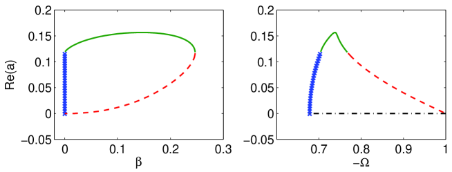
Figure 5: Solutions of (28) and (29) when $D=0$. Left: Re($a$) versus $\beta$. Right: Re($a$) versus $-\Omega$, for $A=0.95$.

Blue crosses indicate the modulated drift state which occurs for $\beta=0,\mbox{Im}(a)=0$. In this state none of the oscillators have synchronised with one another. The green solid line indicates the stable chimera, for which some of the oscillators are synchronised with one another while the remainder drift. The red dashed curve is the unstable chimera. The black dash-dot line represents the uniform drift state for which $\beta=a=0$. Along this line (which has collapsed to a point in the left panel of Fig. 5) all oscillators are synchronised, $\theta_{i}=\theta_{j},\forall i,j$. If $A$ was decreased, the saddle-node bifurcation seen in the left panel of Fig. 5 would move to a lower value of $\beta$. (Note that stability of solutions is inferred, as it was by Abrams and Strogatz [3]. All we have in (28) and (29) are algebraic equations governing the steady states, with no dynamics.)

A similar picture when $D=0.01$ is shown in Fig. 6, with the same conventions. We see that the modulated drift state (which no longer has $\mbox{Im}(a)=0$) has moved away from $\beta=0$, as has the uniform drift state ($a=0$). Although we have not indicated it in Fig. 5, for $D=0$ and $0<\beta$, the synchronised state (with $a=0$) is stable. However for $0<D$ there is now a range of $\beta$ (approximately $0.03<\beta<0.165$ when $D=0.01$) for which the synchronised state is unstable. (This is the extent of the dash-dotted line in the left panel of Fig. 6.) For $\beta$ outside this range, i.e. for $\beta$ small enough or large enough, the synchronised state remains stable.

Comparing the left panels of Fig. 5 and Fig. 6 we see that the case of identical oscillators ($D=0$) is degenerate in the sense that both the modulated and uniform drift states are “hidden” at $\beta=0$, but both occur over finite intervals of $\beta$ when $0<D$.

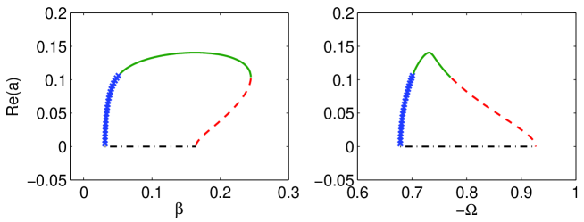
Figure 6: Solutions of (28) and (29) when $D=0.01$. Left: Re($a$) versus $\beta$. Right: Re($a$) versus $-\Omega$, for $A=0.95$.

Fig. 7 shows the results of following the pitchfork and saddle-node bifurcations seen in Fig. 6 as $D$ is varied. Note that the two pitchfork bifurcations emanate from $(D,\beta)=(0,0)$. The rightmost pitchfork bifurcation changes from sub- to super-critical at the termination of the curve of saddle-node bifurcations. For approximately $0.047<D<0.058$ there is no bistability; instead there is a range of $\beta$ values for which only the chimera state is stable. Outside this range only the synchronous state is stable. For $D$ greater than about 0.058 there do not exist any chimera states.

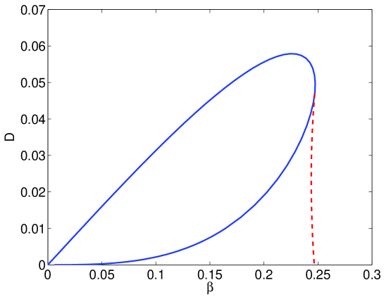
Figure 7: Curves of pitchfork (solid) and saddle-node (dashed) bifurcations of solutions of (28) and (29). Fig. 6 corresponds to a horizontal “slice” through this figure at $D=0.01$. $A=0.95$.

From Fig. 7 we see that with $\beta$ small and fixed, increasing $D$ first destabilises and then restabilises the synchronous state. This is the same behaviour as observed in Fig. 1 for the model (1), and is demonstrated in Fig. 8 where we fix $\beta=0.15$ and successively increase $D$ from 0 to 0.02 to 0.06. For $D=0$ the synchronised state is stable (bottom left panel). At $t\approx 100$ a chimera forms, with the center of the unsynchronised cluster at $i\approx 200$ and the center of the synchronised cluster at $i\approx 700$ (bottom middle panel). Once $D$ is increased above the upper blue curve in Fig. 7 only the (noisy) synchronised state is stable (bottom right panel).

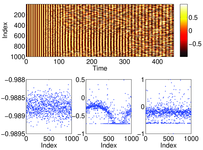
Figure 8: Results of a simulation of (18) for which $D$ is switched from 0 to 0.02 at $t=50$, and then increased to 0.06 at $t=300$. Top: $\sin{\phi_{i}}$. Bottom row: average of $d\phi_{i}/dt$ as a function of index $i$ over the time intervals $[0,50]$ (left), $[150,300]$ (middle) and $[300,450]$ (right). $N=1000,\beta=0.15,A=0.95$.

6.3 Generalisations

As shown in Sec. 4.2, if

$$g(\omega)=\frac{\sqrt{2}D^{3}}{\pi}\left(\frac{1}{\omega^{4}+D^{4}}\right)$$

we could repeat the analysis of (19), obtaining equations similar to, though more complicated than, (28) and (29), still with the unknowns $c,a$ and $\Omega$. Indeed, for any distribution $g$ the double integrals (25) and (26) could be evaluated numerically.

The form of (22) is a direct result of choosing $G$ to have one Fourier mode. If more modes were used in $G$ (if, for example, we were approximating a given coupling function with a finite Fourier series), eqn. (22) would have more terms and thus more coefficients to be found.

6.4 Chimera states and “bumps”

Chimera states as studied in this section are very similar to “bump” states which have been studied in computational neuroscience modelling [12, 11]. The main difference between bump states in neural models and the chimera states studied here is that in neural models, the uncoupled unit is a model neuron which — as an input current is increased — starts to fire periodically once the current has passed a threshold [11], whereas in the chimera states studied here the uncoupled unit is a phase oscillator with uniform angular velocity. In neural models, a bump is a self-consistent state for which some neurons receive subthreshold input (and are thus quiescent) while other receive superthreshold input (and are thus firing). It is the coupling of phase oscillators through a sinusoidal function of the phase itself (as in (20)) which allows some oscillators to lock and rotate at a uniform frequency (which can be set to zero by moving to a rotating coordinate frame), while others drift, and thus a chimera can form.

To further emphasise the similarity, compare Fig. 4 in [11] with the insets in Fig. 12 in [3], and with the middle plot in the bottom row of Fig. 8 (keeping in mind that this is a disordered system). The bifurcations of bumps are also very similar to those of chimerae on a ring — they both typically appear as unstable states bifurcating from a spatially-uniform state; compare Fig. 10 in [12] with Fig. 12 in [3].

7 Summary

We have considered the effects of heterogeneity in the intrinsic frequencies of oscillators on chimera states in Kuramoto-type networks of coupled phase oscillators. Previous authors had only considered these states in networks of identical oscillators [1, 2, 3, 10, 16, 21]. By assuming a Lorentzian distribution of intrinsic frequencies we have generalised the results of Abrams et al. [1] and Abrams and Strogatz [2, 3], obtaining similar equations to them, but with an extra parameter, viz. the width of the Lorentzian distribution. All of our results show that chimerae are robust — within limits — to heterogeneity in their intrinsic frequencies, and we have shown some of the interesting bifurcations that can be induced by such heterogeneity.

Importantly, in light of the recent results of Pikovsky and Rosenblum [18] regarding the validity of the Ott-Antonsen ansatz (6) used in this paper, our numerical results in Sec. 3 support the observation by Martens et al. [14] that this ansatz can be used to study all attractors of a Kuramoto-type system whenever the oscillators have randomly distributed frequencies.

The results presented here rely on the form of the equations studied. In particular, the results in Secs. 2-5 rely on the remarkable recent results of Ott and Antonsen [17] showing that the infinite network can be exactly described by a finite number of ODEs, although not necessarily completely [18]. Similarly, the analysis in Sec. 6 depended on the form of the coupling in (18), through a trigonometric function of phase differences. The challenge remains to discover similar results for oscillators not described by a single variable, and not coupled in this way.

Acknowledgements: I thank the referees for their very helpful comments.

References

- [1] Abrams, D. M., Mirollo, R., Strogatz, S. H., and Wiley, D. A. Solvable model for chimera states of coupled oscillators. Phys. Rev. Lett. 101 (2008), 084103.
- [2] Abrams, D. M., and Strogatz, S. H. Chimera states for coupled oscillators. Phys. Rev. Lett. 93 (2004), 174102.
- [3] Abrams, D. M., and Strogatz, S. H. Chimera states in rings of nonlocally coupled oscillators. Int. J. Bifn. Chaos 16 (2006), 21–37.
- [4] Acebrón, J., Bonilla, L., Pérez Vicente, C., Ritort, F., and Spigler, R. The Kuramoto model: A simple paradigm for synchronization phenomena. Rev. Mod. Phys. 77 (2005), 137–185.
- [5] Baesens, C., Guckenheimer, J., Kim, S., and MacKay, R. Three coupled oscillators: mode-locking, global bifurcations and toroidal chaos. Physica D 49, 3 (1991), 387–475.
- [6] Barreto, E., Hunt, B., Ott, E., and So, P. Synchronization in networks of networks: The onset of coherent collective behavior in systems of interacting populations of heterogeneous oscillators. Phys. Rev. E 77 (2008), 036107.
- [7] Childs, L. M., and Strogatz, S. H. Stability diagram for the forced kuramoto model. arXiv.org:0807.4717.
- [8] Kevrekidis, I., Gear, C., and Hummer, G. Equation-free: The computer-aided analysis of complex multiscale systems. AIChE Journal 50 (2004), 1346–1355.
- [9] Kuramoto, Y. Chemical oscillations, waves, and turbulence. Springer-Verlag, 1984.
- [10] Kuramoto, Y., and Battogtokh, D. Coexistence of Coherence and Incoherence in Nonlocally Coupled Phase Oscillators. Nonlinear Phenom. Complex Syst. 5 (2002), 380 – 385.
- [11] Laing, C., and Chow, C. Stationary Bumps in Networks of Spiking Neurons. Neural Comput. 13 (2001), 1473–1494.
- [12] Laing, C. R. On the application of equation-free modelling to neural systems. J. Comput. Neurosci. 20 (2006), 5 – 23.
- [13] Laing, C. R., and Kevrekidis, I. G. Periodically-forced finite networks of heterogeneous coupled oscillators: a low-dimensional approach. Physica D 237 (2008), 207–215.
- [14] Martens, E. A., Barreto, E., Strogatz, S. H., Ott, E., So, P., and Antonsen, T. M. Exact results for the kuramoto model with a bimodal frequency distribution. arXiv.org:0809.2129.
- [15] Montbrió, E., Kurths, J., and Blasius, B. Synchronization of two interacting populations of oscillators. Phys. Rev. E 70 (2004), 056125.
- [16] Omel chenko, O., Maistrenko, Y., and Tass, P. Chimera States: The Natural Link Between Coherence and Incoherence. Phys. Rev. Lett. 100 (2008), 044105.
- [17] Ott, E., and Antonsen, T. M. Low dimensional behavior of large systems of globally coupled oscillators. Chaos 18 (2008), 037113.
- [18] Pikovsky, A., and Rosenblum, M. Partially integrable dynamics of hierarchical populations of coupled oscillators. arXiv:0809.3700v2.
- [19] Pikovsky, A., Rosenblum, M., and Kurths, J. Synchronization. Cambridge University Press, 2001.
- [20] Ren, L., and Ermentrout, B. Phase locking in chains of multiple-coupled oscillators. Physica D 143, 1-4 (2000), 56–73.
- [21] Sethia, G., Sen, A., and Atay, F. Clustered Chimera States in Delay-Coupled Oscillator Systems. Phys. Rev. Lett. 100 (2008), 144102.
- [22] Singer, W. Neuronal Synchrony: A Versatile Code for the Definition of Relations? Neuron 24 (1999), 49–65.
- [23] Strogatz, S. From Kuramoto to Crawford: exploring the onset of synchronization in populations of coupled oscillators. Physica D 143 (2000), 1–20.
- [24] Strogatz, S. Sync: The Emerging Science of Spontaneous Order. Hyperion, 2003.
- [25] Watanabe, S., and Strogatz, S. Integrability of a globally coupled oscillator array. Physical Review Letters 70 (1993), 2391–2394.
- [26] Watanabe, S., and Strogatz, S. Constants of motion for superconducting Josephson arrays. Physica. D 74 (1994), 197–253.
- [27] Wiesenfeld, K., Colet, P., and Strogatz, S. Synchronization transitions in a disordered josephson series array. Phys. Rev. Lett. 76 (1996), 404–407.