Constraining Cosmology with High Convergence Regions
in Weak Lensing Surveys

Abstract

We propose to use a simple observable, the fractional area of “hot spots” in weak gravitational lensing mass maps which are detected with high significance, to determine background cosmological parameters. Because these high-convergence regions are directly related to the physical nonlinear structures of the universe, they derive cosmological information mainly from the nonlinear regime of density fluctuations. We show that in combination with future cosmic microwave background anisotropy measurements, this method can place constraints on cosmological parameters that are comparable to those from the redshift distribution of galaxy cluster abundances. The main advantage of the statistic proposed in this paper is that projection effects, normally the main source of uncertainty when determining the presence and the mass of a galaxy cluster, here serve as a source of information.

1. Introduction

Weak gravitational lensing (WL), i.e., the coherent distortion of images of faint distant galaxies by the gravitational tidal field of the intervening matter distribution (Tyson, Wenk, & Valdes, 1990), has been established as a powerful cosmological tool [see, e.g., Bartelmann & Schneider (2001) for a review]. Since this effect is purely gravitational, it directly probes the matter distribution along the line of sight, thus providing a way to understand the nature and the evolutionary history of the universe that is relatively insensitive to how light or baryons trace dark matter. Since the earliest measurements of WL by galaxy clusters (Fort et al., 1988; Tyson, Wenk, & Valdes, 1990), WL by large-scale structure, known as “cosmic shear”, has been detected based on optical (Wittman et al., 2000; Van Waerbeke et al., 2000; Bacon, Refregier, & Ellis, 2000; Kaiser, Wilson, & Luppino, 2000) and radio observations (Chang, Refregier, & Helfand, 2004).

Future WL surveys, such as the Large Synoptic Survey Telescope (LSST), will measure the cosmic shear field with great precision over half the sky. Recent attention has focused on how best to extract information from the shear/convergence field in order to constrain cosmological parameters. The primary focus so far has been using the standard two-point statistics (Blandford et al., 1991; Miralda-Escudé, 1991; Kaiser, 1992), which probes the underlying matter power spectrum in projection. In this paper, we propose to use a simple, direct observable: the fraction of high signal-to-noise ratio ($S/N$) points detected in WL surveys, as another discriminator of cosmology. We utilize the results of an N-body simulation to quantify both the theoretical predictions and the observational uncertainties of this statistic.

As is well-known, the common two-point statistics do not contain all the statistical information of the WL convergence field, as the nonlinear gravitational instability induces non-Gaussian signatures in the mass distribution and hence in the WL convergence field as well. Unfortunately, there is no complete statistical analysis in practice for the underlying matter density field in the nonlinear regime. Previous studies of weak lensing statistics on small angular scales, correspondingly, were restricted to the low-order statistics, using the halo model [see, e.g., Cooray & Sheth (2002) for a review], or the “scaling ansatz” (Hamilton et al., 1991), later extended and calibrated by N-body simulations (Jain, Mo, & White, 1995; Peacock & Dodds, 1996; Smith et al., 2003), for the nonlinear evolution of clustering. These low-order statistics include: the two-point correlation function or equivalently the power spectrum, at small scales (Jain & Seljak, 1997), the three-point correlation function or the bispectrum (Takada & Jain, 2003a, b, 2004), the third-order moment: skewness (Bernardeau, van Waerbeke, & Mellier, 1997; Jain & Seljak, 1997; Hui, 1999) and the fourth-order moment: kurtosis (Takada & Jain, 2002). An alternative approach is to use the redshift distribution of nonlinear object abundance (Haiman, Mohr, & Holder, 2001), such as shear-selected galaxy cluster samples (Weinberg & Kamionkowski, 2003; Wang et al., 2004; Fang & Haiman, 2007), using the Press-Schechter prescription (Press & Schechter, 1974; Bond et al., 1991) with calibration by N-body simulations (Sheth & Tormen, 1999; Jenkins et al., 2001). In addition, the “ratio-statistic” (Jain & Taylor, 2003; Bernstein & Jain, 2004; Song & Knox, 2004; Hu & Jain, 2004; Zhang, Hui, & Stebbins, 2005) has been constructed to use the geometrical information from tomographic shear/convergence power spectra on small scales. These analyses have shown that comparable information may be contained in the linear and in the nonlinear regime.

The statistics mentioned above are by no means a full characterization of the convergence field, yet they all face challenges, either from the theoretical or the observational side, which need to be addressed. Including higher-order statistics might give a substantial increase in information, but they are in practice noisy and computationally intensive. To take advantage of the synergy between these statistics, one needs to account for their covariance, which is difficult to calculate analytically. One hope is to run large simulations and directly measure this covariance. Galaxy cluster samples selected optically, by their X-ray flux or by their Sunyaev-Zel’dovich effect signatures, are limited by the uncertain astrophysics when modeling the mass-observable relations and require “self-calibration” (Majumdar & Mohr, 2003; Wang et al., 2004; Lima & Hu, 2005), as the mass function is exponentially sensitive to errors of limiting mass. Shear-selected galaxy clusters, on the other hand, have the advantage that the selection function can be determined ab initio by N-body simulations, since only gravity is involved. However, projection effects result in false detections, missing clusters (White, van Waerbeke, & Mackey, 2002; Hamana, Takada, & Yoshida, 2004; Hennawi & Spergel, 2005), and producing significant uncertainty in the cluster mass derived from the shear signals (Metzler et al., 1999; de Putter & White, 2005), degrading the cosmological information content.

In this paper, we instead focus on the one-point probability distribution function (PDF) of the WL convergence field. There are three main motivations. First, the one-point PDF is a simple yet powerful tool to probe non-Gaussian features, and since the non-Gaussianity in the convergence field is induced by the growth of structure, it holds cosmological information (Reblinsky et al., 1999; Jain, Seljak, & White, 2000; Kruse & Schneider, 2000; Valageas, Munshi, & Barber, 2005). These previous works have shown that the one-point PDF is capable of discriminating cosmologies with different $\Omega_{m}$, such as an open cold dark matter (CDM) model, a flat cosmological constant-dominated ($\Lambda$)-CDM model, and a standard CDM model.

Second, and the primary motivation of this work, is that the fractional area statistic we propose in this paper takes into account projection effects by construction. Determined by the high-convergence tail of the PDF, it is an analog of Press-Schechter formalism, thus similar to the abundance of galaxy clusters but without contamination due to projection effects. This statistic also utilizes information mainly from the nonlinear regime and complements the well-established statistics in the linear regime. The goal of our work is to give a more quantitative assessment of the statistical information in the nonlinear regime (particularly focusing on the properties of dark energy) provided by this fractional area statistic and its complementarity to other probes of cosmology, e.g., the cosmic microwave background (CMB) anisotropies.

Third, besides utilizing the cosmic shear field (Zhang & Pen, 2005) which we will focus on in this paper, there are several other observational techniques which could be used to map out the convergence PDF. For example, with forthcoming large samples of high redshift supernovae from LSST-like or Joint Dark Energy Mission (JDEM)-like surveys, one could measure the magnification distribution of these standard candles due to lensing by the large scale structure in the foreground, and construct the convergence PDF (Dodelson & Vallinotto, 2006; Cooray, Holz, & Huterer, 2006); it is also possible to measure the convergence field through the statistics of cosmic magnification (Jain, 2002), using, for instance, 21cm-emitting galaxies (Zhang & Pen, 2005, 2006).

The rest of this paper is organized as follows. Our basic calculational methodology, including a calibration of the (co)variance using simulation outputs, is described in § 2. Results of using the fractional area statistic for an LSST-like WL survey are presented in § 3, with discussions of its complementarity to other dark energy probes, as well as of various uncertainties. Conclusions and implications of this work are given in § 4. Finally, in a series of appendices, we show the details of our calculations.

2. Calculational Method

2.1. Convergence Field with Gaussian Smoothing

Consider some source galaxies detected in a WL survey, with a redshift distribution of $n(z)$ and a surface density of $n_{g}=\int n(z)dz$. The shear field is measured from the distortion of their images. A convergence field, or sometimes called mass map, can be reconstructed from the shear field (Kaiser & Squires, 1993; Squires & Kaiser, 1996; Bartelmann et al., 1996; Van Waerbeke, Bernardeau & Mellier, 1999), smoothed over scale $\theta_{G}$ with a Gaussian window function $W_{G}(\theta)=\exp(-\theta^{2}/\theta^{2}_{G})/(\pi\theta^{2}_{G})$. This map is a sum of the true, smoothed convergence field and the noise field due to the randomly oriented intrinsic ellipticities of source galaxies:

$$K(\vec{\theta})=\kappa_{(S)}(\vec{\theta})+\kappa_{(N)}(\vec{\theta}).$$ (1)

Both fields are assumed to have zero mean and are statistically isotropic (ensemble average is same along each line of sight).

Under the assumption that the correlation of intrinsic ellipticities and the clustering of the source galaxies can be neglected, and no other systematic errors are present, Van Waerbeke (2000) has shown that the noise field $\kappa_{(N)}$ can be modeled as a Gaussian random field with variance:

$$\sigma^{2}_{(N)}\equiv\langle\kappa_{(N)}^{2}\rangle=\frac{\sigma^{2}_{\epsilon}}{4\pi\theta^{2}_{G}n_{g}},$$ (2)

where $\sigma_{\epsilon}$ is the root-mean-square value of the intrinsic ellipticity of source galaxies. The two-point correlation function of $\kappa_{(N)}$ induced by the smoothing is

$$C_{(N)}(\theta)=\sigma^{2}_{(N)}\exp\left(-\frac{\theta^{2}}{2\theta^{2}_{G}}\right),$$ (3)

where $\theta\equiv|\vec{\theta}_{1}-\vec{\theta}_{2}|$ is the angular separation between two points in the field.

The true convergence field, on the other hand, is essentially non-Gaussian. Its one-point PDF is skew, because $\kappa_{(S)}$ has a minimum value, corresponding to an totally empty path between the source and the observer. The convergence without smoothing, by using Born approximation, is a weighted projection along a particular line of sight of the mass density perturbation field (Bernardeau, van Waerbeke, & Mellier, 1997):

$$\kappa(\vec{\theta})=\int^{\infty}_{0}d\chi\,W_{\rm len}(\chi)\delta(\chi\vec{\theta},\chi),$$ (4)

where $\chi$ is the comoving distance to redshift $z$, and $\delta$ is the over-density at comoving distance $\chi$. Taking $\delta=-1$ everywhere along the line of sight, gives the minimum value of $\kappa_{(S)}$:

$$\kappa_{(S)\rm min}=\kappa_{\rm min}=-\int^{\infty}_{0}d\chi\,W_{\rm len}(\chi),$$ (5)

as the smoothing has no effect on a constant. For a fixed source plane at redshift $z_{s}$ corresponding to $n(z)=n_{g}\delta(z-z_{s})$, the weight function is given by (assuming a flat universe for simplicity):

$$W_{\rm len}(\chi,\chi_{s})=\frac{3}{2}\,\Omega_{m}\left(\frac{H_{0}}{c}\right)^{2}(1+z)\,\chi\left(1-\frac{\chi}{\chi_{s}}\right)\mathcal{H}(\chi_{s}-\chi),$$ (6)

where $\chi_{s}\equiv\chi(z_{s})$ denotes the comoving distance to the source plane and $\mathcal{H}$ is the Heaviside step function. Note that this quantity $\kappa_{\rm min}$, which is a source of the non-Gaussianity of the convergence field, depends on the source redshift and on cosmology. The covariance and the correlation function of the smoothed convergence field, using Limber’s approximation, are given in Appendices A and C as Eq. (C1) and (A3).

Points with high $S/N$ in the convergence field are of both experimental and theoretical interest: not only are they related to the underlying physical density field at high fidelity, but they capture the important features of the nonlinear regime as well. Mathematically, they correspond to the so-called “excursion set”, whose properties have been studied extensively in other similar contexts (most famously to describe the halo mass function, e.g., Bond et al., 1991). For pedagogical purposes, let us consider the excursion set $E_{\nu}$ of the true smoothed convergence field at redshift $z_{s}$, defined as the union of all points with $\kappa_{(S)}>\nu\sigma_{(N)}$ (see § 3 for including the noise field). The fractional area of $E_{\nu}$ is then given by

$$\mathcal{F}(\nu,z_{s})\equiv\frac{A_{\nu}}{A_{\rm tot}}=\frac{1}{A_{\rm tot}}\int d^{2}\vec{\theta}\,\mathcal{H}[\kappa_{(S)}(\vec{\theta},z_{s})-\nu\sigma_{(N)}],$$ (7)

where $A_{\nu}$ is the area of the excursion set $E_{\nu}$, and $A_{\rm tot}$ is the total sky coverage of a survey. $\kappa_{(S)}$ is a statistical quantity, so the fractional area has a mean value of

$$\langle\mathcal{F}(\nu,z_{s})\rangle=\frac{\langle A_{\nu}\rangle}{A_{\rm tot}}=\int_{\nu\sigma_{(N)}}^{\infty}d\kappa_{(S)}\,P_{1}(\kappa_{(S)}),$$ (8)

where $P_{1}$ is the one-point PDF of $\kappa_{(S)}$. The spatial integration cancels with $A_{\rm tot}$ because of the statistical isotropy of the field. Similarly, the fractional area has a variance determined by the two-point PDF, which is given in Appendix C by Eq. (C4).

2.2. Statistical Properties of the True Convergence Field

Let us first focus on the one-point PDF of $\kappa_{(S)}$ at different redshifts: $P_{1}(\kappa_{(S)},z_{s})$, which determines the mean fractional area $\langle\mathcal{F}(\nu,z_{s})\rangle$. Several works have used the “stable-clustering ansatz” (Peebles, 1980) to derive the one-point PDF of the true convergence, with (Valageas, 2000b; Munshi & Jain, 2000; Wang, Holz, & Munshi, 2002) and without (Valageas, 2000a) smoothing, calibrated by N-body simulations. The important conclusion of these works is that there exists a universal one-point PDF, well approximated by a two-parameter family: the variance of the reduced convergence $\langle\kappa^{2}_{(S)}\rangle/\kappa^{2}_{\rm min}$ and the minimum convergence $\kappa_{\rm min}$.

In this section, we concentrate on the constraint equations of the one-point PDF required by the normalization, the mean, and the variance (Das & Ostriker, 2006). By normalizing $\kappa_{(S)}$ to $\kappa^{\prime}=\kappa_{(S)}/|\kappa_{\rm min}|$, the constraints can be written as

$$\int_{-1}^{\infty}d\kappa^{\prime}\,P_{1}(\kappa^{\prime}) = 1,$$

$$\int_{-1}^{\infty}d\kappa^{\prime}\,P_{1}(\kappa^{\prime})\kappa^{\prime} = 0,$$ (9)

$$\int_{-1}^{\infty}d\kappa^{\prime}\,P_{1}(\kappa^{\prime})\kappa^{\prime 2} = \langle\kappa_{(S)}^{2}\rangle/\kappa^{2}_{\rm min}.$$

We consider three different fitting formulae for the one-point PDF of the convergence field from the literature. In the next section, we will use WL simulation outputs to assess the accuracy of the high convergence tail of these three models.

The first model we consider is the log-normal distribution studied in Taruya et al. (2002), and is given by

$$P_{1}(\kappa_{(S)})\,d\kappa_{(S)}=\frac{d\kappa_{(S)}}{|\kappa_{\rm min}|+\kappa_{(S)}}$$ (10)

$$\times\frac{1}{\sqrt{2\pi\sigma^{2}_{LN}}}\exp\left\{-\frac{[\ln(1+\kappa_{(S)}/|\kappa_{\rm min}|)+\sigma^{2}_{LN}/2]^{2}}{2\sigma^{2}_{LN}}\right\}.$$

Only one parameter, $\sigma^{2}_{LN}=\ln{(1+\langle\kappa^{2}_{(S)}\rangle/\kappa^{2}_{\rm min})}$, is needed to satisfy the constraint equations.

The second model is the stretched Gaussian distribution proposed in Wang, Holz, & Munshi (2002),

$$P_{1}(\kappa_{(S)})\,d\kappa_{(S)}=\frac{d\kappa_{(S)}}{|\kappa_{\rm min}|}C_{\rm norm}\exp\left\{-\left[\frac{(1+\kappa_{(S)}/|\kappa_{\rm min}|)-\eta_{\rm peak}}{p(1+\kappa_{(S)}/|\kappa_{\rm min}|)^{q}}\right]^{2}\right\}.$$ (11)

Here we closely follow the original notation, except the PDF is now written in terms of $\kappa_{(S)}$ instead of $\eta\equiv 1+\kappa_{(S)}/|\kappa_{\rm min}|$. As stated earlier, the four fitting parameters $C_{\rm norm}$, $\eta_{\rm peak}$, $p$ and $q$ depend only upon $\langle\kappa^{2}_{(S)}\rangle/\kappa^{2}_{\rm min}$ [see Eq. (8) of Wang, Holz, & Munshi (2002)]. The complication of this model is that there is a need to impose an upper limit of the convergence $\kappa_{\rm max}$ in order to get the correct variance.

The third model takes the form of a modified log-normal distribution as proposed in Das & Ostriker (2006):

$$P_{1}(\kappa_{(S)})\,d\kappa_{(S)}=\frac{d\kappa_{(S)}}{|\kappa_{\rm min}|+\kappa_{(S)}}$$ (12)

$$\times N\exp\left\{-\frac{[\ln(1+\kappa_{(S)}/|\kappa_{\rm min}|)+\Sigma^{2}/2]^{2}[1+A/(1+\kappa_{(S)}/|\kappa_{\rm min}|)]}{2\Sigma^{2}}\right\}.$$

Given $\langle\kappa^{2}_{(S)}\rangle/\kappa^{2}_{\rm min}$, we can uniquely specify $N$, $\Sigma$ and $A$ by numerically solving the three constraint equations. The dependence of these three parameters on the variance is plotted in Figure 2 of Das & Ostriker (2006).

For the analysis in this paper, we emphasize that the cosmological dependence of these PDFs, i.e., information on dark energy, enters only through the variance of the reduced convergence: $\langle\kappa^{2}_{(S)}\rangle/\kappa^{2}_{\rm min}$, and through the minimum: $\kappa_{\rm min}$ as an additional scaling factor.

Once the form of the convergence PDF is specified, the mean fractional area is determined by its integral [Eq. (8)]. The (co)variance of the fractional area for various thresholds and redshifts, $\mathrm{Cov}[\mathcal{F}(\mu,z_{i}),\mathcal{F}(\nu,z_{j})]$, on the other hand, requires knowing the joint two-point PDF of the convergence field, as we can see, e.g., in Eq. (C4). To the best of our knowledge, among the three cases considered above, the two-point function can be computed analytically only in the log-normal model; the results are presented in Appendix C. Note that we do not use the covariance matrix of the log-normal model for our actual calculations – we will instead utilize simulation outputs to directly measure the (co)variance. The results for the log-normal model will be used only for comparison, and to justify extrapolations from simulations, as we discuss in the next section.

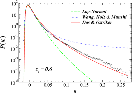
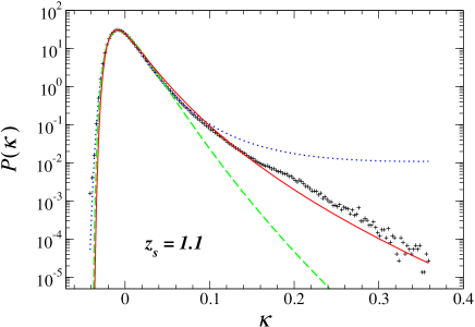
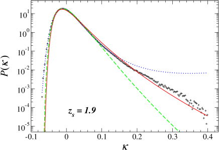
Figure 1.— One-point PDFs of the convergence fields. Three panels correspond to three distinct redshift bins. The cross symbols are (binned) normalized histograms measured directly from the simulation outputs. The three curves in each panel are best-fits to the simulation data using different models as described in the text. Note that the ranges of $x$ and $y$-axes are different for each panel.

2.3. Simulation and Model-Fitting

The simulation outputs we use are those of White (2005). There are a total of 32 convergence fields from two independent N-body simulation runs. Each field is $3\times 3$ deg², divided into $1024\times 1024$ pixels, so that the angular size of a pixel is $\sim$10.5 arcsec. There are three source redshift planes at $z_{s}=0.6$, 1.1, and 1.9 for each field, representing the mean redshift of three source galaxy bins of an LSST-like survey. The cosmological parameters are adopted from first-year measurements by the Wilkinson Microwave Anisotropy Probe (WMAP), as summarized in Table 1 of Spergel et al. (2003): a spatially flat $\Lambda$CDM model with a scale-invariant initial scalar power spectrum ($n_{s}=1$) and present-day normalization $\sigma_{8}=0.9$. The matter density is $\Omega_{m}=0.28$ and the baryon density is $\Omega_{b}=0.049$. The Hubble constant is $H_{0}=70$ km/s/Mpc.

We first apply a Gaussian window function to smooth all the fields, with $\theta_{G}$ chosen to be 1 arcmin ($\sim$ 5.7 pixel):

$$\kappa_{(S)}(i,j)=\displaystyle\sum_{m^{2}+n^{2}\leq 32^{2}}\kappa(i+m,j+n)\exp\left(-\frac{m^{2}+n^{2}}{5.7^{2}}\right)$$

$$\div\sum_{m^{2}+n^{2}\leq 32^{2}}\exp\left(-\frac{m^{2}+n^{2}}{5.7^{2}}\right).$$ (13)

$(i,j)$ and $(m,n)$ are integers used to label the coordinates. For each pixel, we smooth it with nearby pixels within a circle of a 32-pixel radius which is roughly 6 arcmin, as the Gaussian weighting is negligible outside. We discard 32 pixels on each side of the field to avoid possible edge effects, and use only $960\times 960$ pixel² in the center of each smoothed field for the analysis.

In Figure 1, we show fits to the normalized histograms of the smoothed convergence fields for the three different PDFs discuss above (using a bin-size of $\Delta\kappa_{(S)}=0.0025$). As described earlier, for all three models, there are only two parameters to fit: the minimum of the distribution and the variance. For the log-normal model and the model proposed by Das & Ostriker (2006), all fitting parameters are fixed once these two quantities are given. However, for the model proposed by Wang, Holz, & Munshi (2002), there is a further complication in determining $\kappa_{\rm max}$. For this model, we have therefore relaxed the assumption above, and allowed all parameters to vary simultaneously, except we imposed a prior that they lie in the ranges roughly matching Figure 2 in Wang, Holz, & Munshi (2002): $0.6<\eta_{\rm peak}<1$, $0<w<0.5$, and $0.5<q<2.5$.

Recall that the log-normal distribution would be a symmetric parabola on a log-log plot. The actual distribution from simulations, however, is skewed toward the high-$\kappa_{(S)}$ tail [see also Das & Ostriker (2006)], so the log-normal PDF under-predicts the tail of the distribution. In contrast, the Wang, Holz, & Munshi (2002) model over-predicts the distribution in this range, as the distribution is cut at $\kappa_{\rm max}$. Overall, the model by Das & Ostriker (2006) goes through the simulation data points remarkably well at all three redshifts.

A slightly different expression for $\kappa_{\rm min}$ was given in Linder (2007), taking into account density inhomogeneities by applying an extended Dyer-Roder formalism (Dyer & Roeder, 1972, 1973) to a completely empty line of sight [also see Seitz & Schneider (1992)]. The correction to the commonly used Eq. (5) is only large when the sources are at very high redshifts ($10\%$ for our fiducial cosmology at redshift $z=3$). In principle, $\kappa_{\rm min}$ affects the high-tail of the distribution, since it is used to normalize the universal PDF. One could also directly measure this minimum quantity from the simulations. However, the low end of the PDF might be really suppressed, because a completely empty line of sight is extremely unlikely in a finite-size simulation; the smoothing procedure makes it even less probable. We have found that the minimum convergence measured from simulations is nevertheless larger than theoretical predictions, either using Eq. (5) or Linder (2007). The best-fit $\kappa_{\rm min}$ of the Das & Ostriker (2006) model, however, agrees well with the measured minimum value. This is a $\sim 20-50\%$ effect, depending on the source redshift [see a more detailed discussion in Taruya et al. (2002)]. One intriguing question is which, among the minimum values mentioned above, could lead to a more universal PDF? Particular, for the purposes of this paper, which one leads to the most universal high-tail distribution? We hope to investigate this question in future work, using larger-volume simulations with various cosmologies. In this paper, we simply use Eq. (5) to calculate the derivatives of the fractional areas with respect to the cosmological parameters.

To conclude, for the purpose of taking derivatives in the Fisher matrix analysis (see below), we adopt the universal one-point PDF provided by Das & Ostriker (2006), with the variance of the convergence field computed by using the nonlinear matter power spectrum from Smith et al. (2003) as given by Eq. (C1) and the minimum as given by Eq. (5).

Next, we measure directly from the simulation outputs the covariance matrix of the fractional areas with various thresholds and redshifts: ${\rm Cov}[\mathcal{F}(\mu,z_{i}),\mathcal{F}(\nu,z_{j})]$. The variance is given by

$$\mathrm{Var}[\mathcal{F}(\nu,z_{s})]=\frac{1}{N_{f}-1}$$

$$\times\left[\displaystyle\sum_{m=1}^{N_{f}}\left(\frac{N^{(m)}(\nu,z_{s})}{N_{p}}\right)^{2}-\frac{1}{N_{f}}\left(\sum_{m=1}^{N_{f}}\frac{N^{(m)}(\nu,z_{s})}{N_{p}}\right)^{2}\right].$$ (14)

Here $N^{(m)}(\nu,z_{i})$ is the total number of pixels with signal above the threshold $\nu\sigma_{(N)}$, in the $m$-th field at redshift $z_{s}$; $N_{f}=32$ is the total number of fields and $N_{p}=960^{2}$ is the total number of pixels in each field. Similarly, the covariance is given by

$$\mathrm{Cov}[\mathcal{F}(\mu,z_{i}),\mathcal{F}(\nu,z_{j})]=\frac{1}{N_{f}-1}$$ (15)

$$\times\left[\displaystyle\sum_{m=1}^{N_{f}}\frac{N^{(m)}(\mu,z_{i})}{N_{p}}\frac{N^{(m)}(\nu,z_{j})}{N_{p}}-\frac{1}{N_{f}}\sum_{m=1}^{N_{f}}\frac{N^{(m)}(\mu,z_{i})}{N_{p}}\sum_{m=1}^{N_{f}}\frac{N^{(m)}(\nu,z_{j})}{N_{p}}\right].$$

To extrapolate the results we obtain from a 9 deg² simulation field to a 20,000 deg² LSST-like survey, we also measure the covariance matrix as a function of the field size. To do this, we divide each field into several smaller sub-fields. The following cases are considered: $N_{p}=480^{2}$, $240^{2}$, $120^{2}$, $60^{2}$, and $30^{2}$. For each case, we fix $N_{f}=32$. For example, when $N_{p}=480^{2}$, we first use the upper left $480^{2}$ pixel sub-field of all 32 fields to measure the covariance using Eq. (2.3). We repeat the same procedure for the other three sub-fields, and then take the average of the four results.

In Figure 2, we plot the (co)variance of the fractional area, as a function of scale, for different thresholds and redshift bins measured from the simulation outputs. For small fields, we effectively have more realizations to measure the covariance matrix, for which we plot the average. For comparison, we also plot, as dotted curves, the values calculated using the log-normal model.

One expects that when the size of the field $\theta_{\rm max}$ becomes larger than the correlation length of these “biased regions” in the convergence field, the (co)variance scales with respect to the survey size at least as steeply as $\propto A^{-1}_{\rm tot}$ (coinciding with a Poisson-like scaling; see Appendix C). On smaller scales, the slope is generally shallower due to correlations. For example, we can observe this trend analytically in the log-normal case – the covariance is given by a Poisson expression [Eq. (C9)] for large scales and an additional non-Poisson correction term [Eq. (C11)]. The simulation points in Figure 2 show that for low-redshift bins, the scale of 1024 pixel (3 deg) is already within the Poisson region. For higher redshift bins, the slope at 1024 pixel is shallower than Poisson. However, the slope does agree well with the log-normal model, which predicts that the scale of 1024 pixel is very close to the edge of the Poisson region. Thus, for our Fisher matrix analysis, we estimate the covariance matrix of the fractional area for an LSST-like survey by Poisson-scaling the measured value from the simulation outputs with the largest field size of $N_{p}=960^{2}$ pixel. This extrapolation to 20,000 deg² is shown explicitly in Figure 2 as the solid curves. The justification for this extrapolation, using the log-normal model, is admittedly still somewhat heuristic, but measurements of the covariance out to larger scales require larger size simulations; we defer this to future work.

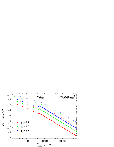
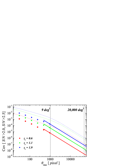
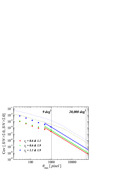
Figure 2.— The top left panel shows the variance $\mathrm{Var}[\mathcal{F}(\mu=2,z_{i})]$ within three distinct redshift bins; the top right panel shows the covariance $\mathrm{Cov}[\mathcal{F}(\mu=2,z_{i}),\mathcal{F}(\nu=2.5,z_{i})]$ within the same three redshift bins. The bottom panel shows $\mathrm{Cov}[\mathcal{F}(\mu=2,z_{i}),\mathcal{F}(\nu=2,z_{j})]$ across three different pairs of redshift bins. All symbols in each panel show results measured directly from the simulation outputs. The solid curves show the estimate of the covariance matrix through Poisson-extrapolation, which we use in the actual calculations. The dotted curves are calculated using the log-normal model, which are plotted only for comparison.

2.4. Random Ellipticity Noise

In order to incorporate the presence of noise into our forecasts, we start with the simplest case: modeling the noise due to the intrinsic ellipticity as a two-dimensional Gaussian random field that is uncorrelated with the signal (Van Waerbeke, 2000; Jain & van Waerbeke, 2000). We use a Gaussian random number generator with zero-mean and a variance of $\sigma_{(N)}$ to generate noise fields and co-add onto the original convergence fields. We adopt $\sigma_{\epsilon}=0.3$, $\theta_{G}=1$ arcmin, and $n_{g}=40/3$ arcmin^-2 (the denominator “3” reflects the redshift binning) in Eq. (2) for an LSST-like survey, thus $\sigma_{(N)}\sim 0.023$. We then repeat the same Gaussian smoothing procedure and measure the covariance matrix of the fractional area. In this case, the one-point PDF is simply a convolution of the original distribution and the Gaussian PDF.

Modeling of the noise field as above might be overly simplified, even in the case when all other systematics are absent. This is because Van Waerbeke (2000) only worked in the WL limit, in which the estimator of the convergence is safely linear. We here typically use a signal threshold of several times $\sigma_{(N)}$, reaching values of order $\sim 5-10\%$. Construction of the convergence field from the observed reduced shear is nonlinear, and therefore gets non-negligible higher-order corrections, which will complicate the expression for the convergence error. Besides the intrinsic ellipticity, there will be other systematic effects, due to the point spread function, mirror distortion, etc, which will increase the scatter, and may produce an unknown bias in measuring the cosmic shear.

In our analysis, we adopt an approach similar to what has been done in the literature for cluster counts in order to account for the uncertainties of the mass-observable relations (Majumdar & Mohr, 2003; Wang et al., 2004; Lima & Hu, 2005). We still make the simple assumption that the overall convergence noise is Gaussian and uncorrelated with the signal, but with unknown variance and bias, which will be included as additional nuisance parameters that are fit by the survey itself, simultaneously with the cosmology parameters (“self-calibration”). We assign the variance and bias in each redshift bin as free parameters, and their fiducial values are $\{\sigma_{(N)},\kappa_{\rm bias}\}=\{0.023,0\}$, chosen to be same for all redshift bins. For WL power spectrum and bispectrum tomography, Huterer et al. (2006) have shown that there is sufficient information in these statistics themselves to successfully self-calibrate additive and multiplicative shear systematics. As we will see below, the nuisance parameters we consider here likewise do not significantly degrade the cosmological constraints derived from the one-point statistic, provided we have some external knowledge of what the intrinsic ellipticity distribution is. The reason for this is essentially that the PDF contains both the tomographic and the shape information (similarly to the case of cluster counts, where the nuisance parameters cannot simultaneously mimic changes in both the shape and the $z$-dependence of the mass function caused by variations in cosmology).

2.5. Error Forecasts

The usual Fisher matrix technique (Tegmark, Taylor, & Heavens, 1997) is employed to assess the cosmological sensitivity of the fractional area statistic. This method allows a quick exploration of the parameter space and gives a lower bound to the statistical uncertainty of each model parameter to be fit by future experimental data.

We consider a WL survey with specifications similar to that planned for LSST: a sky coverage of $A_{\rm tot}=20,000$ deg², source galaxies with the redshift distribution adopted from Eq. (18) in Song & Knox (2004), normalized to a total surface number density of $n_{g}=40$ arcmin^-2, and the intrinsic ellipticity dispersion $\sigma_{\epsilon}=0.3$. The galaxies are divided into three bins with mean redshift $z_{s}=0.6$, 1.1 and 1.9 so that each bin contains the same number of galaxies. The Gaussian smoothing is taken over the scale $\theta_{G}=1$ arcmin within the nonlinear regime. Seven different $S/N$ thresholds, from $\nu=2.0$ to $5.0$ in increment of $\Delta\nu=0.5$, are considered simultaneously for each redshift bin to utilize the information contained in the shape of the PDF (see § 3 below for discussions of different choices of smoothing scale and $S/N$ thresholds).

The full Fisher matrix is given by Eq. (15) of Tegmark, Taylor, & Heavens (1997):

$$F_{\alpha\beta}=\frac{1}{2}\mathrm{Tr}\left[{\bf C}^{-1}{\bf C}_{,\alpha}{\bf C}^{-1}{\bf C}_{,\beta}+{\bf C}^{-1}\left({\vec{\mathcal{F}}}_{,\alpha}{\vec{\mathcal{F}}}^{t}_{,\beta}+{\vec{\mathcal{F}}}_{,\beta}{\vec{\mathcal{F}}}^{t}_{,\alpha}\right)\right]~{},$$ (16)

where ${\vec{\mathcal{F}}}$ is the list of mean fractional areas above different thresholds and at different redshifts, arranged into a vector, and ${\bf C}$ is the covariance matrix between them. We have used the standard comma notation for derivatives.

In this paper, we neglect the cosmological dependence of the covariance matrix, i.e. the sample variance. It is straightforward to spell out the last two terms, which gives

$$F_{\alpha\beta} = \frac{1}{2}\mathrm{Tr}\left[{\bf C}^{-1}\left({\vec{\mathcal{F}}}_{,\alpha}{\vec{\mathcal{F}}}^{t}_{,\beta}+{\vec{\mathcal{F}}}_{,\beta}{\vec{\mathcal{F}}}^{t}_{,\alpha}\right)\right]={\vec{\mathcal{F}}}^{t}_{,\alpha}{\bf C}^{-1}{\vec{\mathcal{F}}}_{,\beta}$$ (17)

$$= \sum_{i,j}\sum_{\mu,\nu}\frac{\partial\langle\mathcal{F}(\mu,z_{i})\rangle}{\partial p_{\alpha}}({\bf C}^{-1})_{(\mu,i)(\nu,j)}\frac{\partial\langle\mathcal{F}(\nu,z_{j})\rangle}{\partial p_{\beta}},$$

where $p_{\alpha}$ includes the cosmological parameters of interest, as well as possible nuisance parameters. The set of different redshift bins and $S/N$ thresholds are labeled by $i$ or $j$, and $\mu$ or $\nu$, respectively.

The covariance matrix ${\bf C}$ is estimated by extrapolation from simulations, as discussed above. Note that in Eq. (17), this covariance matrix is needed only for the fiducial cosmology. The subscript “$(\mu,i)(\nu,j)$” denotes the corresponding matrix element. The choice of cumulative $S/N$ thresholds instead of independent bins is made to simplify the calculations in the Appendices. Note that the off-diagonal terms of the covariance matrix, reflecting the cross-correlations between different redshift bins and $S/N$ thresholds, are nonzero so that double-counting information from overlapping lens redshift and $S/N$ ranges is avoided.

We consider a spatially flat cosmological model with seven parameters. The fiducial values are close to those adopted in the simulations: $\{\Omega_{\rm DE},w_{0},w_{a},\Omega_{m}h^{2},\Omega_{b}h^{2},\sigma_{8},n_{s}\}=$ $\{0.72,-1,0,0.137,0.024,0.9,1\}$ (note a higher $\sigma_{8}$ than WMAP three-year result). The dark energy equation of state is parametrized as (Chevallier & Polarski, 2001; Linder, 2003)

$$w(a)=w_{0}+w_{a}(1-a)=w_{0}+w_{a}\frac{z}{1+z}.$$ (18)

CMB anisotropies have played a crucial role in firmly establishing the current “standard model” of cosmology (Spergel et al., 2003, 2007). To take advantage of the future high precision data which will be available from planned CMB anisotropy measurements, a survey with specifications similar to the Planck surveyor (Planck) is considered. The Fisher matrix for the CMB temperature and polarization anisotropies is constructed as given in Wang et al. (2004).

Table 1Calibrated Cosmological Parameter Constraints from LSST using the fractional area statistic and adding Planck priors: $\Delta\Omega_{m}h^{2}=0.0012$, $\Delta\Omega_{b}h^{2}=0.00014$, and $\Delta n_{s}=0.035$. For the pessimistic scenario, we adopt $1\%$ priors on the additive and multiplicative errors already achieved by current surveys. For the optimistic scenario, we adopt $0.01\%$ and $0.05\%$ priors on the additive and multiplicative error respectively, which is the goal of future surveys.

Parameter Constraints LSST ($\mathcal{F}$) LSST ($\mathcal{F}$) + Planck (priors)   Pessimistic   $\Delta w_{p}$ 0.094 0.022   $z_{p}$ 0.50 0.94   $\Delta w_{0}$ 0.55 0.12   $\Delta w_{a}$ 1.6 0.25   $\Delta\Omega_{\rm DE}$ 0.046 0.0095   $\Delta\sigma_{8}$ 0.047 0.0080   Optimistic   $\Delta w_{p}$ 0.028 0.012   $z_{p}$ 0.60 0.60   $\Delta w_{0}$ 0.16 0.043   $\Delta w_{a}$ 0.42 0.11   $\Delta\Omega_{\rm DE}$ 0.015 0.0038   $\Delta\sigma_{8}$ 0.031 0.0029

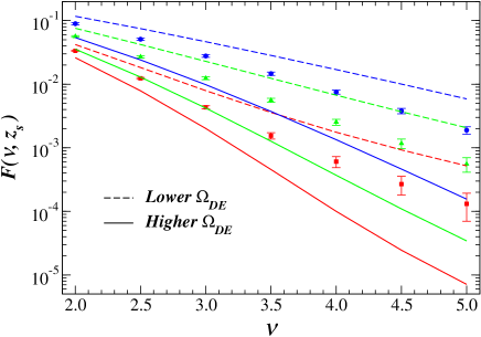
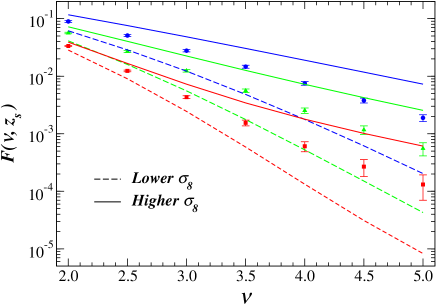
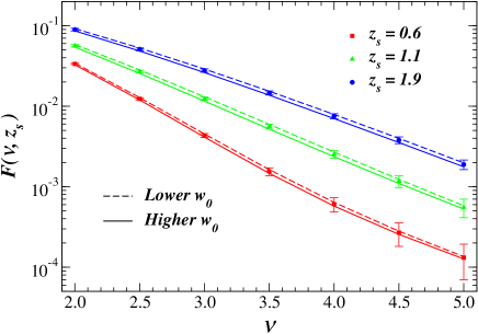
Figure 3.— Mean fractional area $\langle\mathcal{F}\rangle$ for different S/N threshold $\nu$, different redshift $z_{s}$, and its dependence on various cosmological parameters. The symbols in each panel show $\langle\mathcal{F}\rangle$ in the fiducial cosmology (with the intrinsic ellipticity noise taken into account), with the error bars measured directly from the simulations. Note that the error bars are correlated, and they are also enlarged by a factor of 10 to be clearly visible. The solid (dashed) curves show results when the given cosmological parameter is $20\%$ higher (lower) than its fiducial value.

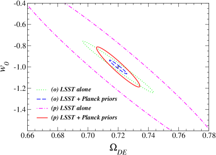
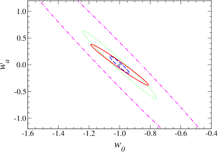
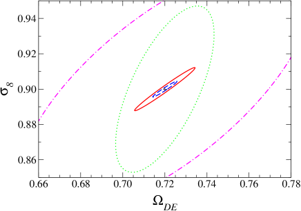
Figure 4.— Constraints on various cosmological parameters from an LSST-like weak lensing survey. The $68\%$ C.L. contours in all panels show reasonable optimistic and pessimistic estimates including systematic errors for an LSST-like survey, with or without priors from a Planck-like CMB survey. The pessimistic scenario corresponds to the additive and multiplicative errors already achieved by current surveys. The optimistic scenario corresponds to the accuracy goal of future surveys, such as LSST. Different contours are for LSST alone (dotted curve) and LSST with priors from Planck (dashed curve) in the optimistic scenario; LSST alone (dot-dashed curve) and with Planck priors (solid curve) in the pessimistic scenario. The contours are marginalized over all other relevant parameters.

3. Results and Discussion

Before we present the results, it is useful to keep several numbers in mind. The variance of the noise field $\sigma_{(N)}\sim 0.023$ due to the intrinsic ellipticities of the source galaxies is the same for each redshift bin; the variance of the true smoothed convergence field $\sigma_{(S)}$ is $\sim 0.009$, 0.017 and 0.025 for $z_{s}=0.6$, 1.1 and 1.9 respectively. The lowest threshold $2\sigma_{(N)}$ is chosen so that the points considered are all in the tail of the underlying PDF: $\kappa_{(S)}(\vec{\theta})>\sigma_{(S)}$. The reason for restricting ourselves to the tail instead of using the full PDF is that the points which lie within $1\sigma_{(S)}$ of the mean probe the linear regime, where the shear field can be well approximated as Gaussian. In this regime the power spectrum, which has already been studied extensively, should contain essentially all of the statistical information.

Figure 3 shows how the fractional area statistic depends on the cosmological parameters $\Omega_{\rm DE},\sigma_{8}$ and $w_{0}$. The data points in each panel are the fractional areas above different thresholds for each redshift bin in the fiducial cosmology. The lines are calculated by varying the parameter in question by $\pm 20\%$ (and leaving all other parameters unchanged). For reference, we have also shown, as the error bars, the variance measured directly from the simulations. The dependencies revealed on this figure make intuitive sense: decreasing $\Omega_{\rm DE}$ (or equivalently, increasing $\Omega_{m}$), increasing $\sigma_{8}$, or making $w_{0}$ more negative all affect the growth of structures in the direction of having larger amplitudes, which increase the shear.

Table 1 summarizes our main results for an LSST-like survey alone, as well as its combination with Planck. We follow the “self-calibration” approach, in which we assume $\sigma_{(N)}$ and $\kappa_{\rm bias}$ are unknown, and fit separately in each redshift bin. To account for the uncertainties of the six extra nuisance parameters, instead of three $S/N$ bins, we utilize seven bins extending from $\nu=2.0$ to $\nu=5.0$ in increments of $\Delta\nu=0.5$. We consider two scenarios for the convergence systematics: the top half of Table 1 shows a rather pessimistic projection of the survey, where we adopt $1\%$ priors on $\sigma_{(N)}$ and $\kappa_{\rm bias}$, corresponding to the additive and multiplicative errors already achieved by current surveys (Fu et al., 2008); the bottom half of Table 1 represents a more optimistic projection of an LSST-like survey, where we adopt a $0.01\%$ prior on $\sigma_{(N)}$ and a $0.05\%$ prior on $\kappa_{\rm bias}$, which is the accuracy goal of future surveys. Note that in the last column, we adopt a conservative approach and only include independent priors on $\Omega_{m}h^{2}$, $\Omega_{b}h^{2}$, and $n_{s}$ (the diagonal approximation instead of the full CMB Fisher matrix). These three parameters are expected to be constrained by Planck alone to $0.9\%$, $0.6\%$ and $0.4\%$ respectively (Hu, 2002).

As noted above, the cosmological dependence of the fractional areas, similar to galaxy cluster abundance, comes in through two quantities: (1) the variance of the reduced convergence, $\langle\kappa^{2}\rangle/\kappa^{2}_{\rm min}$, thus most sensitive to the amplitude of the density fluctuation $\sigma_{8}$; (2) the minimum value of the convergence, $\kappa_{\rm min}$, thus most sensitive to the matter content $\Omega_{m}$, or $\Omega_{\rm DE}$ as a flat universe is assumed. However, the fractional-area statistic also provides good constraints on the dark energy equation of state, for the following reason. With Planck priors for $\Omega_{m}h^{2}$, $\Omega_{b}h^{2}$, and $n_{s}$, which are all below the $1\%$ level, an LSST-like survey can determine $\Omega_{\rm DE}$ and $\sigma_{8}$ very well (to a few percent accuracy) by using the fractional area statistic, which in turn breaks the degeneracies in the growth of structure between these two parameters and the dark energy equation of state parameters: $w_{0}$ and $w_{a}$.

We follow the Dark Energy Task Force (DETF) report (Albrecht et al., 2006) and calculate the pivot scale-factor $a_{p}$, or equivalently the pivot redshift $z_{p}$, where the dark energy equation of state $w(a)$ is best constrained. In the pessimistic case, we find $\Delta w_{p}=0.022$ with $a_{p}=0.52$ ($z_{p}=0.94$) for LSST with Planck prior, where $w_{p}\equiv w(a_{p})$. This is improved to $\Delta w_{p}=0.012$ with $a_{p}=0.63$ ($z_{p}=0.60$) in the optimistic case. The corresponding “figure of merit” is $(\Delta w_{p}\Delta w_{a})^{-1}\sim 180$ for the pessimistic projection, which is at the interesting level [compared to the various stage-III experiments; see Albrecht et al. (2006, page 77)], and 760 for the optimistic scenario; the best-constrained pivot point is also at somewhat higher redshift than other proposed probes, which gives a different degeneracy direction on the $w_{0}$-$w_{a}$ plane, so we expect good synergy between the fractional area statistic and other dark energy probes. It is also different from the main degeneracy direction for CMB anisotropies, the angular diameter distance degeneracy, which gives $a_{p}=0.72$ ($z_{p}=0.38$) for our fiducial cosmology.

In Figure 4, we show the two-dimensional marginalized error contours of various cosmological parameters. As shown in the bottom panel, there is still a strong degeneracy between $\Omega_{\rm DE}$ (or equivalently $\Omega_{m}$, as we have assumed a flat universe) and $\sigma_{8}$ in the self-calibration case. Consequently, this degrades the constraints of $w_{0}$ and $w_{a}$ by large factors, as shown in the upper panels of Figure 4. We have found that, comparing the pessimistic scenario with the optimistic one, there is respectively, a factor of 2 and 2.5 degradation for the constraint on $w_{p}$ and $w_{a}$ (when Planck priors are added; the degradation is more significant for the convergence-statistic only case). As illustrated by Huterer et al. (2006), the prior information of the intrinsic ellipticity noise can help to restore the dark energy constraints. We also note that the prospects for self-calibration of systematic errors of an LSST-like WL survey would be further improved if the extra information from the tomographic power spectrum or bispectrum were added in the analysis.

The numbers quoted above should be interpreted as the lower bound of the cosmological sensitivities one can get from an LSST-like survey using the statistics described (with Planck priors). In reality, various systematics have to be considered, which we discuss next.

For an LSST-like survey, most of the source galaxies will only have photometric redshift information. To check the sensitivity of the fractional area statistic to the redshift uncertainties, we calculated the change in the source redshift which would cause a shift of the fractional area by more than its $1\sigma$ error. It is estimated using $\Delta z_{s}=(d\langle\mathcal{F}\rangle/dz_{s})^{-1}\times$ $\sqrt{\mathrm{Var}[\mathcal{F}(z_{s})]}$, where $d\langle\mathcal{F}\rangle/dz_{s}$ is the derivative of the mean fractional area with respect to source redshift. We have found that the systematic error (bias) of photometric redshift of the source galaxies needs to be below $0.002$ for low redshift and $0.01$ for $z>2$, which is within the expectations of LSST [see assumption in Ma, Hu, & Huterer (2006); Huterer et al. (2006)]. The requirement on the photometric redshift scatter will not be a major problem, because many source galaxies for each redshift bin are needed to reconstruct the convergence field.

There are also several theoretical uncertainties about the use of the fractional area statistic. One important issue is the theoretical understanding of the one-point PDF of the smoothed convergence field. Similar to the case of the universal halo mass function, the one-point PDF has not been tested extensively for different cosmologies. For instance, the expression given by Das & Ostriker (2006), though in excellent agreement with N-body simulations, has only been checked for one flat $\Lambda$CDM cosmology with $\Omega_{m}=0.3$. As the above discussion indicates, the theoretical prediction for the PDF has to be accurate at the $\sim$ 1 percent level. It is conceivable that the universality might break down at this precision. However, the one-point PDF is such a simple statistic and its derivation adds almost no extra computational cost, once WL simulations are made. We expect our work will inspire currently on-going or planned large WL simulations to obtain accurately calibrated formulas for the PDF.

The baryons can cool and collapse into dense regions, which changes the matter distribution within the virialized objects. The effect on the two-point statistics has been shown to be significant (White, 2004; Zhan & Knox, 2004; Jing et al., 2006; Rudd, Zentner, & Kravtsov, 2007), and will therefore have to be modeled in the interpretation of future WL surveys. This baryonic effect would also alter the PDF tail, and thus the fractional area statistic, especially when small smoothing angles are used. However, Zentner, Rudd, & Hu (2007) have shown that it is possible to take into account this uncertainty through “self-calibration”, i.e., constraining simultaneously the dark energy properties and the uncertain halo profile due to baryonic physics, e.g., halo concentration. We hope to explore the utility of a similar self-calibration technique for the one-point statistic, using the halo model approach (Kruse & Schneider, 2000) in the future.

The mass-sheet degeneracy of weak lensing is not an uncertainty for the fractional area statistic. Because the full PDF is measured, any offset can be determined as the mean should be zero. Besides, one can in principle use the one-point PDF of the filtered tangential shear (Valageas, Munshi, & Barber, 2005) directly instead of the convergence PDF.

It is also important to compare the fractional area statistic with other WL statistics. We have found that the fractional area statistic, in combination with CMB anisotropy measurements, may be able to reach a cosmological sensitivity closely approaching those from using a sample of $\sim 200,000$ shear-selected galaxy clusters (Wang et al., 2004). The two methods are very similar and related in practice, as the majority of the high $S/N$ points are candidates for being real galaxy clusters (Reblinsky et al., 1999; Jain & van Waerbeke, 2000; Weinberg & Kamionkowski, 2003). The most important gain for our approach is that projection effects are not a contamination, since they depend on cosmology, and therefore serve as a source of information instead. The fractional area statistic does not suffer from the missing or false cluster problem, which is indeed the main motivation of this work. The trade-off, however, is that counting the number of clusters as a function of redshift plays a crucial role to constrain the evolution of dark energy, while the convergence field is a two-dimensional projection of all the structures along the line of sight. The tomography of the source galaxies does help, but the broad lensing kernel entangles the information from a wide range of redshifts; tomography is also limited by the number of faint galaxies detected within each redshift bin (in order to reconstruct a convergence field that is not shot-noise dominated).

The WL power spectrum tomography (Song & Knox, 2004; Zhan, 2006) and the bispectrum tomography (Takada & Jain, 2004) have been shown to be very powerful cosmological probes and sensitive to the evolution of dark energy. For example, Zhan (2006) find that an LSST-like survey can deliver constraints of $\Delta w_{0}\sim 0.16$ and $\Delta w_{a}\sim 0.36$ from lensing alone. The fractional area statistic must include additional information from higher order statistics, because the one-point PDF is determined by all orders of cumulants (Balian & Schaeffer, 1989). Furthermore, in analogy with cluster counts, the fractional area statistic is helped by the exponential sensitivity of the tail of the PDF to the cosmological parameters. The scale information, imprinted in different multipole moments of power spectrum, can be retrieved with different smoothing scales for the fractional area statistic: the linear regime of the power spectrum should be recovered by using various larger smoothing angular scales and the nonlinear regime by smaller scales. However, unlike in Fourier space where different modes are independent, using different smoothing scales in real space produces mass maps that are correlated with each other. In this work, we only utilize one particular smoothing scale $\theta_{G}=1$ arcmin, which is within the nonlinear regime. As mentioned earlier, in the linear regime, most of the statistical information is already contained in the two-point correlation function. Interesting future work includes studying how to correctly take advantage of the information from the scale-dependence of the fractional area statistic, and its complementarity to other WL statistics.

Finally, we note that the fractional area statistic is known as the first Minkowski functional. In the two-dimensional case, there are two other functionals: the length and the genus of the excursion set. These three Minkowski functionals, which are additive and are invariant under translations as well as rotations, completely characterize the morphological properties of the high convergence regions. These functionals have been extensively studied for CMB as useful tests of the Gaussianity of the primordial density perturbation field [see, e.g., Winitzki & Kosowsky (1998)]. Since the convergence field is definitely non-Gaussian, including the other two functionals which depend on derivatives of the convergence field must yield additional cosmological information (Taruya et al., 2002; Guimarães, 2002).

4. Conclusions

We have shown that, in future wide field weak gravitational lensing surveys, a simple one-point statistic – the total fractional area of high $S/N$ points in the convergence field – is a promising probe of cosmology. It is sensitive to the total matter content of the universe and the amplitude of the density fluctuations, which helps breaking the intrinsic degeneracies in the growth of structure between cosmological parameters, thus constraining the properties of dark energy.

The main conclusion of this work is that the fractional area statistic provides constraints on cosmological parameters similar to the redshift distribution of galaxy cluster abundance, but without suffering from the projection effects. Indeed, the statistic is explicitly constructed to take advantage of projections as part of the signal.

We expect the fractional area statistic will help achieve the goal of “precision cosmology” and shed light on the mystery of dark energy.

Appendix A Limber’s Approximation

In this section, the two-point cross-correlation function (CCF) and auto-correlation function (ACF) of the true convergence field are calculated by using Limber’s approximation. Note that the calculations below do not require the log-normal assumption.

The cross-power spectrum of the convergence field on two different source planes at $z_{i}$ and $z_{j}$, both with Gaussian smoothing, is related to the three-dimensional matter power spectrum $P_{\delta}(k)$ by the Fourier space analogue of Limber’s equation (Kaiser, 1992):

$$\hat{P}_{(S)}(k_{\bot})=\int^{\infty}_{0}d\chi\,\frac{W_{\rm len}(\chi,\chi_{i})W_{\rm len}(\chi,\chi_{j})}{\chi^{2}}P_{\delta}\left(\frac{k_{\bot}}{\chi},\chi\right)\tilde{W}^{2}_{G}(k_{\bot}\theta_{G}),$$ (A1)

where $\chi_{i}\equiv\chi(z_{i})$; $W_{\rm len}(\chi,\chi_{i})$ is given by Eq. (6); $\tilde{W}_{G}(x)=\exp(-x^{2}/4)$ is the Fourier transform of the Gaussian smoothing window function; $k_{\bot}$ denotes the Fourier modes perpendicular to the line of sight, which are the only contribution to the projected power under Limber’s approximation.

The CCF is then the Fourier transform of the cross-power spectrum:

$$\hat{C}_{(S)}(\theta)\equiv\langle\kappa_{(S)}(\vec{\theta}_{1},z_{i})\kappa_{(S)}(\vec{\theta}_{2},z_{j})\rangle=\int^{\infty}_{0}d\chi\,W_{\rm len}(\chi,\chi_{i})W_{\rm len}(\chi,\chi_{j})\left[\pi\int^{\infty}_{0}dk^{\prime}_{\bot}\,\frac{\Delta^{2}(k^{\prime}_{\bot},z)}{k^{\prime\,2}_{\bot}}J_{0}(k^{\prime}_{\bot}\chi\theta)\tilde{W}^{2}_{G}(k^{\prime}_{\bot}\chi\theta_{G})\right],$$ (A2)

where we have changed variable $k^{\prime}_{\bot}=k_{\bot}/\chi$. Here $\Delta^{2}(k,z)=4\pi k^{3}P_{\delta}(k,z)/(2\pi)^{3}$ is the dimensionless nonlinear power spectrum, which is calculated as in Smith et al. (2003); $J_{0}$ denotes the Bessel function of order 0; $\theta\equiv|\vec{\theta}_{1}-\vec{\theta}_{2}|$ is the angular separation of two field points.

The auto-power spectrum and the ACF of $\kappa_{(S)}$ are special cases of the expressions above when $i=j$:

$$P_{(S)}(k_{\bot}) = \int^{\infty}_{0}d\chi\,\frac{W_{\rm len}^{2}(\chi,\chi_{s})}{\chi^{2}}P_{\delta}\left(\frac{k_{\bot}}{\chi},\chi\right)\tilde{W}^{2}_{G}(k_{\bot}\theta_{G}),$$

$$C_{(S)}(\theta) = \int^{\infty}_{0}d\chi\,W_{\rm len}^{2}(\chi,\chi_{s})\left[\pi\int^{\infty}_{0}dk^{\prime}_{\bot}\,\frac{\Delta^{2}(k^{\prime}_{\bot},z)}{k^{\prime\,2}_{\bot}}J_{0}(k^{\prime}_{\bot}\chi\theta)\tilde{W}^{2}_{G}(k^{\prime}_{\bot}\chi\theta_{G})\right].$$ (A3)

Appendix B Log-normal Random Field

There is one specific class of non-Gaussian random fields of theoretical interest, which can be related in some functional way to one or several Gaussian random fields [see, e.g., Coles & Barrow (1987); also see Bardeen et al. (1986) and Bond & Efstathiou (1987) for a general introduction of Gaussian random field]. The useful feature of these non-Gaussian fields is that when the functional form of this mapping is known, the statistical properties are analytically determined from the underlying Gaussian fields.

A log-normal random field is the one for which the mapping from a Gaussian random field and the inverse are given by

$$\kappa = F_{LN}(\alpha)=|\kappa_{\rm min}|\left[\exp\left(\sigma^{~{}}_{LN}\alpha-\frac{\sigma^{2}_{LN}}{2}\right)-1\right],$$

$$\alpha = F^{-1}_{LN}(\kappa)=\frac{1}{\sigma_{LN}}\left[\ln(1+\frac{\kappa}{|\kappa_{\rm min}|})+\frac{\sigma^{2}_{LN}}{2}\right],$$ (B1)

where $\alpha$ is a Gaussian field with zero mean and unit variance. The minimum of the distribution $\kappa_{\rm min}$ and the variance $\sigma^{2}_{LN}\equiv\ln(1+\langle\kappa^{2}\rangle/\kappa^{2}_{\rm min})$ are needed in order to specify $\kappa$. Some relevant statistical properties of the log-normal field $\kappa$ are listed below:

1. The one-point PDF of a log-normal field $\kappa$ is obtained from the corresponding Gaussian PDF of $\alpha$ by simply changing variable:

   $$P_{1}(\kappa)\,d\kappa=\frac{1}{\sqrt{2\pi\sigma^{2}_{LN}}}\exp\left\{-\frac{[\ln(1+\kappa/|\kappa_{\rm min}|)+\sigma^{2}_{LN}/2]^{2}}{2\sigma^{2}_{LN}}\right\}\frac{d\kappa}{|\kappa_{\rm min}|+\kappa}.$$ (B2)

2. The two-point CCF of two log-normal fields $\kappa$ and $\kappa^{\prime}$ is obtained by using the joint two-point PDF of the underlying Gaussian fields $\alpha$ and $\alpha^{\prime}$:

   $$P_{2}[\alpha,\alpha^{\prime};\hat{C}_{G}(\theta)]\,d\alpha d\alpha^{\prime} = \frac{e^{-Q_{2}/2}}{\sqrt{(2\pi)^{2}[1-\hat{C}^{2}_{G}(\theta)]}}\,d\alpha d\alpha^{\prime},$$

   $$Q_{2} = \frac{1}{1-\hat{C}^{2}_{G}(\theta)}[\alpha^{2}-2\hat{C}_{G}(\theta)\alpha\alpha^{\prime}+\alpha^{\prime 2}],$$ (B3)

   where $\hat{C}_{G}(\theta)\equiv\langle\alpha(\vec{\theta}_{1})\alpha^{\prime}(\vec{\theta}_{2})\rangle$ is the CCF of $\alpha$ and $\alpha^{\prime}$; $\theta$ is the angular separation. Carrying out the average gives the relation between these two CCF’s:

   $$\hat{C}(\theta) \equiv \langle\kappa(\vec{\theta}_{1})\kappa^{\prime}(\vec{\theta}_{2})\rangle=\exp[\sigma^{~{}}_{LN}\sigma^{\prime}_{LN}\hat{C}_{G}(\theta)]-1,$$

   $$\hat{C}_{G}(\theta) = \frac{1}{\sigma^{~{}}_{LN}\sigma^{\prime}_{LN}}\ln[1+\hat{C}(\theta)].$$ (B4)

3. The relation between the two-point ACF of a log-normal field and the underlying Gaussian field is a special case of the expression above when $\kappa^{\prime}$ is just $\kappa$:

   $$C(\theta) = \exp[\sigma^{2}_{LN}C_{G}(\theta)]-1,$$

   $$C_{G}(\theta) = \frac{1}{\sigma^{2}_{LN}}\ln[1+C(\theta)],$$ (B5)

   where $C$ and $C_{G}$ are the two-point ACF’s of $\kappa$ and $\alpha$ respectively. When $\theta=0$, $C(0)=\langle\kappa^{2}\rangle/\kappa^{2}_{\rm min}$ thus $C_{G}(0)=\langle\alpha^{2}\rangle=1$ as expected.

Appendix C Statistical Properties of the Fractional Area

In this section, we want to calculate the covariance matrix in Eq. (17) by assuming that the convergence field with Gaussian smoothing can be approximately described by a log-normal random field $\kappa_{(S)}(\alpha)=F_{LN}(\alpha)$. To specify the function $F_{LN}$, the parameter $\kappa_{\rm min}$ is given by Eq. (5) and the other parameter $\sigma^{2}_{LN}$ can be calculated using Eq. (A3):

$$\kappa_{\rm min} = -\int^{\infty}_{0}d\chi\,W_{\rm len}(\chi,\chi_{s}),$$

$$\langle\kappa^{2}_{(S)}\rangle=C_{(S)}(0) = \int^{\infty}_{0}d\chi\,W_{\rm len}^{2}(\chi,\chi_{s})\left[\pi\int^{\infty}_{0}dk^{\prime}_{\bot}\,\frac{\Delta^{2}(k^{\prime}_{\bot},z)}{k^{\prime\,2}_{\bot}}\tilde{W}^{2}_{G}(k^{\prime}_{\bot}\chi\theta_{G})\right],$$ (C1)

as $J_{0}(0)=1$. Note that they both depend on the source redshift $z_{s}$. The CCF of the underlying Gaussian field (similarly for ACF) is obtained by using Eq. (B4), where $\hat{C}(\theta)$ is now $\hat{C}_{(S)}(\theta)$ as given in Eq. (A2).

The mean fractional area of the excursion set $E_{\nu}$ under the log-normal assumption is given by

$$\langle\mathcal{F}(\nu,z_{s})\rangle=\frac{1}{2}\mathrm{erfc}\left(\frac{x_{\nu}}{\sqrt{2}}\right),$$ (C2)

where erfc is the complementary error function; $x_{\nu}\equiv F^{-1}_{LN}(\nu\sigma_{(N)})$ is the effective threshold for $\alpha$.

The covariance between the fractional area with threshold of $\mu$ at redshift $z_{i}$ and the one with threshold of $\nu$ at $z_{j}$ is given by

$$\mathrm{Cov}[\mathcal{F}(\mu,z_{i}),\mathcal{F}(\nu,z_{j})]=\frac{1}{A^{2}_{\rm tot}}\left(\langle A_{\mu}A_{\nu}\rangle-\langle A_{\mu}\rangle\langle A_{\nu}\rangle\right),$$ (C3)

where the statistical average is taken by using the joint two-point PDF as given in Eq. (B3). Because the two-point PDF only depends on the angular separation $\theta$ between two different lines of sight, one spatial integral can be eliminated and gives

$$\mathrm{Cov}[\mathcal{F}(\mu,z_{i}),\mathcal{F}(\nu,z_{j})] = \frac{1}{A_{\rm tot}}\int^{\theta_{\rm max}}_{0}2\pi\theta\,d\theta\int_{\mu\sigma_{(N)}}^{\infty}d\kappa_{1(S)}(z_{i})\int_{\nu\sigma_{(N)}}^{\infty}d\kappa_{2(S)}(z_{j})\,P_{2}[\kappa_{1(S)}(z_{i}),\kappa_{2(S)}(z_{j});\theta]-\langle\mathcal{F}(\mu,z_{i})\rangle\langle\mathcal{F}(\nu,z_{j})\rangle$$ (C4)

$$= \frac{1}{A_{\rm tot}}\int^{\theta_{\rm max}}_{0}2\pi\theta\,d\theta\left\{\int_{x_{\mu}}^{\infty}d\alpha_{i}\int_{x_{\nu}}^{\infty}d\alpha_{j}\,P_{2}[\alpha_{i},\alpha_{j};\hat{C}_{G}(\theta)]-\langle\mathcal{F}(\mu,z_{i})\rangle\langle\mathcal{F}(\nu,z_{j})\rangle\right\},$$

where we have moved the $\langle\mathcal{F}\rangle\langle\mathcal{F}\rangle$ term inside the integral over $\theta$, since it has no dependence on $\theta$; $x_{\mu}$ and $x_{\nu}$ are the effective thresholds of $\alpha_{i}$ and $\alpha_{j}$ respectively as defined in Eq. (C2).

Let us denote

$$\langle\mathcal{F}_{2}[\mu,z_{i};\nu,z_{j};\hat{C}_{G}(\theta)]\rangle=\int^{\infty}_{x_{\mu}}d\alpha_{i}\int^{\infty}_{x_{\nu}}d\alpha_{j}\,P_{2}[\alpha_{i},\alpha_{j};\hat{C}_{G}(\theta)].$$ (C5)

The special case of this expression with $\mu=\nu$ and $i=j$, had been extensively studied (Kaiser, 1984; Politzer & Wise, 1984; Jensen & Szalay, 1986; Kashlinsky, 1991) to approximate the correlation function of “biased regions”, e.g., galaxy clusters. Evaluation of this integral hinges on the equality (Hamilton, Gott, & Weinberg, 1986; Winitzki & Kosowsky, 1998)

$$\frac{\partial\langle\mathcal{F}_{2}(\hat{C}_{G})\rangle}{\partial\hat{C}_{G}}=P_{2}[x_{\mu},x_{\nu};\hat{C}_{G}],$$ (C6)

which can be proven by Fourier transforming the integrand $P_{2}$, then integrating over $\alpha$’s and Fourier transforming back. This first-order ordinary differential equation has a boundary condition that, when $\hat{C}_{G}=0$, the two-point PDF reduces to the product of two independent one-point PDF. Then the double integral can be separated and gives

$$\langle\mathcal{F}_{2}(\mu,z_{i};\nu,z_{j};0)\rangle=\langle\mathcal{F}(\mu,z_{i})\rangle\langle\mathcal{F}(\nu,z_{j})\rangle.$$ (C7)

Thus the term in the curly braces of Eq. (C4) is simply

$$\langle\mathcal{F}_{2}[\mu,\nu;z_{i},z_{j};\hat{C}_{G}(\theta)]\rangle-\langle\mathcal{F}_{2}(\mu,\nu;z_{i},z_{j};0)\rangle=\int^{\hat{C}_{G}(\theta)}_{0}dC^{\prime}\,P_{2}(x_{\mu},x_{\nu};C^{\prime}).$$ (C8)

Substituting the above expression into Eq. (C4), and changing the order of integration by assuming $\hat{C}_{G}(\theta)$ is monotonic, we get:

$$\mathrm{Cov}[\mathcal{F}(\mu,z_{i}),\mathcal{F}(\nu,z_{j})]=\frac{1}{A_{\rm tot}}\int^{\hat{C}_{G}(0)}_{0}dC^{\prime}\,\frac{\hat{\theta}^{2}(C^{\prime})}{2\sqrt{1-C^{\prime 2}}}\exp\left[-\frac{x^{2}_{\mu}-2C^{\prime}x_{\mu}x_{\nu}+x^{2}_{\nu}}{2(1-C^{\prime 2})}\right].$$ (C9)

Here $\hat{\theta}(C^{\prime})$ is the inverse of the CCF: $\hat{C}_{G}(\theta)$ between $\alpha$’s as given in Eq. (B4). The covariance reduces to the variance when $\mu=\nu$ and $z_{i}=z_{j}$:

$$\mathrm{Var}[\mathcal{F}(\nu,z_{s})]=\frac{1}{A_{\rm tot}}\int^{C_{G}(0)}_{0}dC^{\prime}\,\frac{\theta^{2}(C^{\prime})}{2\sqrt{1-C^{\prime 2}}}\exp\left(-\frac{x^{2}_{\nu}}{1+C^{\prime}}\right),$$ (C10)

where $\theta(C^{\prime})$ is the inverse of the ACF: $C_{G}(\theta)$ as given in Eq. (B5). These integrals are finite as long as the CCF/ACF falls off faster than $\theta^{-2}$ at large distances.

We have also assumed $\hat{C}_{G}(\theta_{\rm max})\sim 0$, i.e., the size of the field $\theta_{\rm max}$ is large enough compared with the correlation length of the convergence field [see Eq. (D3)]. The correction term of Eq. (C9) is

$$\Delta(\mathrm{Cov})=\int^{\hat{C}_{G}(\theta_{\rm max})}_{0}dC^{\prime}\,\frac{1-\hat{\theta}^{2}(C^{\prime})/\theta^{2}_{\rm max}}{2\pi\sqrt{1-C^{\prime 2}}}\exp\left[-\frac{x^{2}_{\mu}-2C^{\prime}x_{\mu}x_{\nu}+x^{2}_{\nu}}{2(1-C^{\prime 2})}\right].$$ (C11)

Appendix D Random Noise Field

In the simplest case where the noise due to intrinsic ellipticity and signal are independent of each other, the one-point PDF of the noisy convergence field $K=\kappa_{(S)}+\kappa_{(N)}$ is just a convolution of the log-normal and Gaussian distribution. So the mean fractional area of the excursion set $E_{\nu}$ with $K>\nu\sigma_{(N)}$ is

$$\langle\mathcal{F}(\nu,z_{s})\rangle=\int_{-\infty}^{+\infty}\frac{d\kappa_{(N)}}{\sqrt{2\pi\sigma^{2}_{(N)}}}\exp\left[-\frac{(\kappa_{(N)}-\kappa_{\rm bias})^{2}}{2\sigma^{2}_{(N)}}\right]\,\frac{1}{2}\mathrm{erfc}\left(\frac{x_{\nu}}{\sqrt{2}}\right),$$ (D1)

where the effective threshold $x_{\nu}\equiv F^{-1}_{LN}(\nu\sigma_{(N)}-\kappa_{(N)})$ now depends on the integral variable $\kappa_{(N)}$. We define $F^{-1}_{LN}(\kappa)=-\infty$ when $\kappa\leq\kappa_{\rm min}$. We also allow a nonzero mean of the noise field $\kappa_{\rm bias}$ as in the self-calibration case.

Similarly for the covariance, the integral in Eq. (C5) will be taken over two more variables due to the noise field. The expression involves a five-dimensional integral which, unfortunately, cannot be simplified as what is done in the noise-free case and is very messy. Thus it is useful to get an upper bound of the covariance for this general case as in Winitzki & Kosowsky (1998). Note that in the limit when $x_{\mu}$ or $x_{\nu}$ goes to $-\infty$, $\langle\mathcal{F}_{2}\rangle$ is simply $\langle\mathcal{F}\rangle$. Since the two-point PDF $P_{2}$ is always non-negative, we get $\langle\mathcal{F}_{2}\rangle\leq\min[\langle\mathcal{F}(\mu,z_{i})\rangle,\langle\mathcal{F}(\nu,z_{j})\rangle]$. By using this inequality, the integrand of Eq. (C4) then has no $\theta$ dependence. Therefore,

$$\mathrm{Cov}[\mathcal{F}(\mu,z_{i}),\mathcal{F}(\nu,z_{j})]\leq\frac{\pi\theta^{2}_{c}}{A_{\rm tot}}\langle\mathcal{F}\rangle_{<}(1-\langle\mathcal{F}\rangle_{>}),$$ (D2)

where the subscript “$<$” (or “$>$”) denotes the smaller (or larger) one between two $\langle\mathcal{F}\rangle$’s. The correlation length $\theta_{c}$ is the scale beyond which the correlation can be neglected for physical reasons and is defined as (Bond & Efstathiou, 1987)

$$\theta^{2}_{c}\equiv\frac{\langle K^{2}\rangle}{\langle(\nabla K)^{2}\rangle}=\frac{\langle\kappa^{2}_{(S)}\rangle+\langle\kappa^{2}_{(N)}\rangle}{\langle(\nabla\kappa_{(S)})^{2}\rangle+\langle(\nabla\kappa_{(N)})^{2}\rangle},$$ (D3)

where the variances of the derivative fields are given by

$$\langle(\nabla\kappa_{(S)})^{2}\rangle = -\nabla^{2}C_{(S)}(0)=\int^{\infty}_{0}d\chi\,\chi^{2}W_{\rm len}^{2}(\chi,\chi_{s})\left[\pi\int^{\infty}_{0}dk^{\prime}_{\bot}\,\Delta^{2}(k^{\prime}_{\bot},z)\tilde{W}^{2}_{G}(k^{\prime}_{\bot}\chi\theta_{G})\right],$$

$$\langle(\nabla\kappa_{(N)})^{2}\rangle = -\nabla^{2}C_{(N)}(0)=\frac{2\sigma^{2}_{(N)}}{\theta^{2}_{G}},$$ (D4)

as $\nabla^{2}J_{0}(\theta)=-J_{0}(\theta)$. We again assume $\theta_{\rm max}\gg\theta_{c}$ here.

References

- Albrecht et al. (2006) Albrecht, A., et al. 2006, arXiv:astro-ph/0609591
- Bacon, Refregier, & Ellis (2000) Bacon, D. J., Refregier, A. R., & Ellis, R. S. 2000, MNRAS, 318, 625
- Balian & Schaeffer (1989) Balian, R., & Schaeffer, R. 1989, A&A, 220, 1
- Bardeen et al. (1986) Bardeen, J. M., Bond, J. R., Kaiser, N. & Szalay, A. S. 1986, ApJ, 304, 15
- Bartelmann et al. (1996) Bartelmann, M., Narayan, R., Seitz, S. & Schneider, P. 1996, ApJ, 464, L115
- Bartelmann & Schneider (2001) Bartelmann, M., & Schneider, P. 2001, Phys. Rep., 340, 291
- Bernardeau, van Waerbeke, & Mellier (1997) Bernardeau, F., van Waerbeke, L., & Mellier, Y. 1997, A&A, 322, 1
- Bernstein & Jain (2004) Bernstein, G., & Jain, B. 2004, ApJ, 600, 17
- Blandford et al. (1991) Blandford, R. D., Saust, A. B., Brainerd, T. G., & Villumsen, J.V. 1991, MNRAS, 251, 600
- Bond et al. (1991) Bond, J. R., Cole, S., Efstathiou, G., & Kaiser, N. 1991, ApJ, 379, 440
- Bond & Efstathiou (1987) Bond, J. R., & Efstathiou, G. 1987, MNRAS, 226, 665
- Chang, Refregier, & Helfand (2004) Chang, T.-C., Refregier, A., & Helfand, D. J. 2004, ApJ, 617, 794
- Chevallier & Polarski (2001) Chevallier, M., & Polarski, D. 2001, Int. J. Mod. Phys. D, 10, 213
- Coles & Barrow (1987) Coles, P., & Barrow, J. D. 1987, MNRAS, 228, 407
- Cooray, Holz, & Huterer (2006) Cooray, A., Holz, D. E., & Huterer, D. 2006, ApJ, 637, 77
- Cooray & Sheth (2002) Cooray, A., & Sheth, R. K. 2002, Phys. Rep., 372, 1
- Das & Ostriker (2006) Das, S., & Ostriker, J. P. 2006, ApJ, 645, 1
- de Putter & White (2005) de Putter, R., & White, M. 2005, NewA, 10, 676
- Dodelson (2004) Dodelson, S. 2004, Phys. Rev. D, 70, 023008
- Dodelson & Vallinotto (2006) Dodelson, S., & Vallinotto, A. 2006, Phys. Rev. D, 74, 063515
- Dyer & Roeder (1972) Dyer, C. C., & Roeder, R. C. 1972, ApJ, 174, L115
- Dyer & Roeder (1973) Dyer, C. C., & Roeder, R. C. 1973, ApJ, 180, L31
- Fang & Haiman (2007) Fang, W., & Haiman Z. 2007, Phys. Rev. D, 75, 043010
- Fort et al. (1988) Fort, B., et al. 1988, A&A, 200, 17
- Fu et al. (2008) Fu, L., et al. 2008, A&A, 479, 9
- Guimarães (2002) Guimarães, A. C. C. 2002, MNRAS, 337, 631
- Haiman, Mohr, & Holder (2001) Haiman, Z., Mohr, J. J., & Holder, G. P. 2001, ApJ, 553, 545
- Hamana, Takada, & Yoshida (2004) Hamana, T., Takada, M., & Yoshida, N. 2004, MNRAS, 350, 893
- Hamilton, Gott, & Weinberg (1986) Hamilton, A. J. S., Gott, J. R., & Weinberg, D. H. 1986, ApJ, 309, 1
- Hamilton et al. (1991) Hamilton, A. J. S., Matthews, A., Kumar, P., & Lu, E. 1991, ApJ, 374, 1
- Hennawi & Spergel (2005) Hennawi, J. F., & Spergel, D. N. 2005, ApJ, 624, 59
- Hu (2002) Hu, W. 2002, Phys. Rev. D, 65, 023003
- Hu & Jain (2004) Hu, W., & Jain, B. 2004, Phys. Rev. D, 70, 043009
- Hui (1999) Hui, L. 1999, ApJ, 519, 9
- Huterer et al. (2006) Huterer, D., Takada, M., Bernstein, G. & Jain, B. 2006, MNRAS, 366, 101
- Jain (2002) Jain, B. 2002, ApJ, 580, L3
- Jain, Mo, & White (1995) Jain, B., Mo, H. J., & White, S. D. M. 1995, MNRAS, 276, 25
- Jain & Seljak (1997) Jain, B., & Seljak, U. 1997, ApJ, 484, 560
- Jain, Seljak, & White (2000) Jain, B., Seljak, U., & White, S. D. M. 2000, ApJ, 530, 547
- Jain & van Waerbeke (2000) Jain, B., & van Waerbeke, L. 2000, ApJ, 530, L1
- Jain & Taylor (2003) Jain, B., & Taylor, A. 2003, Phys. Rev. Lett., 91, 141302
- Jenkins et al. (2001) Jenkins, A., et al. 2001, MNRAS, 321, 372
- Jensen & Szalay (1986) Jensen, L. G., & Szalay, A. S. 1986, ApJ, 305, L5
- Jing et al. (2006) Jing, Y. P., et al. 2006, ApJ Lett., 640, L119
- Kaiser (1984) Kaiser, N. 1984, ApJ, 284, L9
- Kaiser (1992) Kaiser, N. 1992, ApJ, 388, 272
- Kaiser & Squires (1993) Kaiser, N., & Squires, G. 1993, ApJ, 404, 441
- Kaiser, Wilson, & Luppino (2000) Kaiser, N., Wilson, G., & Luppino, G. A. 2000, arXiv:astro-ph/0003338
- Kashlinsky (1991) Kashlinsky, A. 1991, ApJ, 376, L5
- Kruse & Schneider (2000) Kruse, G., & Schneider, P. 2000, MNRAS, 318, 321
- Lima & Hu (2005) Lima, M., & Hu, W. 2005, Phys. Rev. D, 72, 043006
- Linder (2003) Linder, E. V. 2003, Phys. Rev. Lett., 90, 091301
- Linder (2007) Linder, E. V. 2008, JCAP, 03, 019
- Ma, Hu, & Huterer (2006) Ma, Z., Hu, W., & Huterer, D. 2006, ApJ, 636, 21
- Majumdar & Mohr (2003) Majumdar, S., & Mohr, J. J. 2003, ApJ, 585, 603
- Metzler et al. (1999) Metzler, C. A., White, M., Norman, M., & Loken, C. 1999, ApJ, 520, 9
- Miralda-Escudé (1991) Miralda-Escudé, J. 1991, ApJ, 380, 1
- Munshi & Jain (2000) Munshi, D., & Jain, B. 2000, MNRAS, 318, 109
- Peacock & Dodds (1996) Peacock, J. A., & Dodds, S. J. 1996, MNRAS, 280, 19
- Peebles (1980) Peebles, P. J. E. 1980, The Large-Scale Structure of the Universe (Princeton: Princeton Univ. Press)
- Politzer & Wise (1984) Politzer, H. D., & Wise, M. D. 1984, ApJ, 285, L1
- Press & Schechter (1974) Press, W., & Schechter, P. 1974, ApJ, 187, 425
- Reblinsky et al. (1999) Reblinsky, K., Kruse, G., Jain, B., & Schneider, P. 1999, A&A, 351, 815
- Rudd, Zentner, & Kravtsov (2007) Rudd, D. H., Zentner, A. R., & Kravtsov, A. V. 2008, ApJ, 672, 19
- Seitz & Schneider (1992) Seitz, S., & Schneider, P. 1992, A&A, 265, 1
- Sheth & Tormen (1999) Sheth, R. K., & Tormen, G. 1999, MNRAS, 308, 119
- Smith et al. (2003) Smith, R. E., et al. 2003, MNRAS, 341, 1311
- Song & Knox (2004) Song, Y.-S., & Knox, L. 2004, Phys. Rev. D, 70, 063510
- Spergel et al. (2003) Spergel, D. N., et al. 2003, ApJ Suppl. Ser. 148, 175
- Spergel et al. (2007) Spergel, D. N., et al. 2007, ApJ Suppl. Ser. 170, 377
- Squires & Kaiser (1996) Squires, G., & Kaiser, N. 1996, ApJ, 473, 65
- Takada & Jain (2002) Takada, M., & Jain, B. 2002, MNRAS, 337, 875
- Takada & Jain (2003a) Takada, M., & Jain, B. 2003, ApJ, 583, 49
- Takada & Jain (2003b) Takada, M., & Jain, B. 2003, MNRAS, 340, 580
- Takada & Jain (2004) Takada, M., & Jain, B. 2004, MNRAS, 348, 897
- Taruya et al. (2002) Taruya, A., et al. 2002, ApJ, 571, 638
- Tegmark, Taylor, & Heavens (1997) Tegmark, M., Taylor, A. N., & Heavens, A. F. 1997, ApJ, 480, 22
- Tyson, Wenk, & Valdes (1990) Tyson, J. A., Wenk, R. A., & Valdes, F. 1990, ApJ, 349, 1
- Valageas (2000a) Valageas, P. 2000, A&A, 354, 767
- Valageas (2000b) Valageas, P. 2000, A&A, 356, 771
- Valageas, Munshi, & Barber (2005) Valageas, P., Munshi, D., & Barber, A. J. 2005, MNRAS, 356, 386
- Van Waerbeke, Bernardeau & Mellier (1999) Van Waerbeke, L., Bernardeau, F., & Y. Mellier 1999, A&A, 342, 15
- Van Waerbeke (2000) Van Waerbeke, L. 2000, MNRAS, 313, 524
- Van Waerbeke et al. (2000) Van Waerbeke, L., et al. 2000, A&A, 358, 30
- Wang et al. (2004) Wang, S., Khoury, J., Haiman, Z., & May, M. 2004, Phys. Rev. D, 70, 123008
- Wang, Holz, & Munshi (2002) Wang, Y., Holz, D. E., & Munshi, D. 2002, ApJ, 572, 15
- Weinberg & Kamionkowski (2003) Weinberg, N. N., & Kamionkowski, M. 2003, MNRAS, 341, 251
- White (2004) White, M. 2004, Astropart. Phys., 22, 211
-
White (2005)
White, M. 2005, Astropart. Phys., 23, 349
(http://mwhite.berkeley.edu/Lensing/Thousand) - White, van Waerbeke, & Mackey (2002) White, M., van Waerbeke, L., & Mackey, J. 2002, ApJ, 575, 640
- Winitzki & Kosowsky (1998) Winitzki, S., & Kosowsky, A. 1998, NewA, 3, 75
- Wittman et al. (2000) Wittman, D. M., et al. 2000, Nature, 405, 143
- Zentner, Rudd, & Hu (2007) Zentner, A. R., Rudd, D. H., & Hu, W. 2008, Phys. Rev. D, 77, 043507
- Zhan (2006) Zhan, H. 2006, J. Cosmol. Astropart. Phys., 8, 8
- Zhan & Knox (2004) Zhan, H., & Knox, L. 2004, ApJ Lett., 616, L75
- Zhang, Hui, & Stebbins (2005) Zhang, J., Hui, L., & Stebbins, A. 2005, ApJ, 635, 806
- Zhang & Pen (2005) Zhang, P., & Pen, U.-L. 2005, Phys. Rev. Lett., 95, 241302
- Zhang & Pen (2006) Zhang, P., & Pen, U.-L. 2006, MNRAS, 367, 169
- Zhang & Pen (2005) Zhang, T.-J., & Pen, U.-L. 2005, ApJ, 635, 821