Small-$x$ single-particle distributions in jets from the coherent branching formalism

Abstract:

We calculate single parton distributions inside quark and gluon jets within the coherent branching formalism, which resums leading and next-to-leading logarithmic contributions. This formalism is at the basis of the modified leading logarithmic approximation (MLLA), and it conserves energy exactly. For a wide preasymptotic range of the evolution variable $Y=\ln\left[E\theta/Q_{0}\right]$, we find marked differences in the shape and norm of single parton distributions calculated in the MLLA or in the coherent branching formalism, respectively. For asymptotically large values $Y\geq 5-10$, the difference in norm persists, while differences in shape disappear. In this way, our numerical study delineates the jet energy scale needed for a reliable application of both approaches. We also study the dependence of the single parton distributions on the hadronization scale $Q_{0}$ and on $\Lambda_{\rm QCD}$, and we calculate within the coherent branching formalism the identified quark and gluon distributions inside quark and gluon jets.

1 Introduction

Since the early days of QCD, it has been known that destructive interference between soft gluon emissions within a jet suppresses hadron production at small values of the momentum fraction $x=p_{h}/E$. For inclusive single-parton distributions, this is seen already in the double logarithmic approximation (DLA), which predicts a hump-backed plateau [1]. However, if one considers the kinematic regime of sufficiently small momentum fractions $x$, and sufficiently large jet energies $E$, where $\ln\left[1/x\right]\sim\ln\left[E/Q_{0}\right]\sim{\cal O}\left(1/\sqrt{\alpha_{s}}\right)$, then corrections to the asymptotic DLA result are of relative order $\sqrt{\alpha_{s}}$ for the peak position of the hump-backed plateau [1, 2, 3]. These corrections remain sizable up to the highest experimentally accessible jet energies. The coherent parton branching formalism [4, 5] leads to evolution equations for the inclusive single- and multi-parton intra-jet distributions, which contain the complete set of next-to-leading ${\cal O}(\sqrt{\alpha_{s}})$ corrections, as well as a subset of higher order corrections. The modified leading logarithmic approach (MLLA) [5, 6] to inclusive parton distributions, which is at the basis of many phenomenological comparisons, can be obtained from these evolution equations after further approximations.

One may ask whether the evolution equations of the coherent branching formalism contain more physics than MLLA. This idea is not supported by parametric considerations, since both MLLA and the original evolution equations are complete up to the same order in $\sqrt{\alpha_{s}}$. However, the idea is supported by kinematic considerations, since the original evolution equations conserve energy exactly, while MLLA does not. This has motivated in recent years several works which aim at going beyond MLLA. In particular, in an approach referred to as NMLLA [7, 8, 9], one keeps all terms of the original evolution equations, which are one order ${\cal O}(\sqrt{\alpha_{s}})$ higher than the MLLA accuracy. In the same manner also ${\cal O}(\alpha_{s})$ corrections to MLLA have been calculated [10, 11]. On the other hand, one may solve the original evolution equations numerically without any further approximation. So far, this has been done for fully integrated partonic jet multiplicities only [12, 13]. The main result of the present work is to solve these original evolution equations for the inclusive single-parton distributions, and to compare the numerical results to those of MLLA.

In the remainder of this introduction, we recall two issues which come up if one compares data to the QCD calculations reviewed above. First, the range of applicability of the evolution equations is limited to sufficiently high energies, and a full numerical solution will allow us to be quantitative about the scale above which a comparison of the formalism with data may be regarded as being reliable. Second, it has been emphasized repeatedly that the QCD prediction for the hump-backed plateau of the single inclusive distribution remains unaffected by the non-perturbative hadronization process as long as hadronization is sufficiently local so that it does not alter significantly the shapes of partonic momentum distributions. In particular, the phenomenologically successful comparison of the (rescaled) partonic MLLA prediction with inclusive hadronic distributions has been viewed as support for a local parton-hadron duality (LPHD) underlying the hadronization mechanism [14, 15]. On the other hand, hadronization models employed e.g. in Monte Carlo event generators, such as the Lund string fragmentation or cluster hadronization lead to a significant further softening of single-inclusive distributions during hadronization [16, 17, 18]. Any difference between MLLA, NMLLA and the exact numerical solution to the evolution equations in the coherent branching formalism may point to the possible relevance of further higher-order and/or non-perturbative effects, and may thus add to our picture of the hadronization process.

The paper is organized as follows. In Sec. 2, we introduce the equations of the coherent branching formalism [4, 5] and we define all quantities of interest. In particular, we discuss in Sec. 2.1 the general ansatz for the initial conditions of these equations. The MLLA approach is briefly recalled in Sec. 2.2. In Sec. 2.3 we describe how we solve the full evolution equations of the coherent branching formalism. The numerical solutions are discussed in Sec. 3. In Sec. 3.1, we present the single-particle spectra in the phenomenologically accessible as well as in the asymptotic range of jet energies. In Sec. 3.2 we show the results for total multiplicity and total energy of partons. In Sec. 3.3 we study the dependence of these results on the hadronization scale. In Sec. 3.4, we explore finally to what extent characteristic differences between the coherent branching formalism and MLLA remain, if one allows for the freedom of adapting the norm and hadronization scale independently in both approaches. Our method of solving the equation of the coherent branching formalism enables us also to determine separately the distributions of quarks and gluons in a quark or a gluon jet. The corresponding results are discussed in Sec. 4. Our conclusions are summarized in Sec. 5.

2 Evolution equations for single parton distributions at small $x$

We want to calculate the single distributions $D_{q}(x,Y)$ and $D_{g}(x,Y)$ of partons in a quark or gluon jet, respectively. Here, $x=p/E$ is the jet momentum fraction of partons, and the variable

$$Y=\ln\frac{E\theta}{Q_{0}}$$ (1)

is written in terms of the sufficiently small jet opening angle $\theta$, and the hadronic scale $Q_{0}$. We denote the logarithm of the momentum fraction by

$$l=\ln\frac{1}{x}\,.$$ (2)

In the coherent parton branching formalism, the evolution equations for these distributions are given by [4, 5]

$$\partial_{Y}D_{q}(x,Y) = \frac{1}{2}\int_{z_{-}}^{z_{+}}dz\,\frac{\alpha_{s}(k^{2}_{\perp})}{\pi}\,$$

$$\hskip 28.45274pt\times\Bigg{\{}P_{qq}(z)\,\bigg{[}D_{q}\Big{(}\frac{x}{z},Y+\ln z\Big{)}+D_{g}\Big{(}\frac{x}{1-z},Y+\ln(1-z)\Big{)}-D_{q}(x,Y)\bigg{]}$$

$$\hskip 34.14322pt+\,P_{gq}(z)\,\bigg{[}D_{g}\Big{(}\frac{x}{z},Y+\ln z\Big{)}+D_{q}\Big{(}\frac{x}{1-z},Y+\ln(1-z)\Big{)}-D_{q}(x,Y)\bigg{]}\Bigg{\}},$$

$$\partial_{Y}D_{g}(x,Y) = \frac{1}{2}\int_{z_{-}}^{z_{+}}dz\,\frac{\alpha_{s}(k^{2}_{\perp})}{\pi}\,$$

$$\hskip 28.45274pt\times\Bigg{\{}P_{gg}(z)\,\bigg{[}D_{g}\Big{(}\frac{x}{z},Y+\ln z\Big{)}+D_{g}\Big{(}\frac{x}{1-z},Y+\ln(1-z)\Big{)}-D_{g}(x,Y)\bigg{]}$$

$$\hskip 28.45274pt+\,2n_{f}\,P_{qg}(z)\,\bigg{[}D_{q}\Big{(}\frac{x}{z},Y+\ln z\Big{)}+D_{q}\Big{(}\frac{x}{1-z},Y+\ln(1-z)\Big{)}-D_{g}(x,Y)\bigg{]}\Bigg{\}},$$

with the unregularized splitting functions

$$P_{qq}(z) = C_{F}\frac{1+z^{2}}{1-z},$$

$$P_{gg}(z) = 2C_{A}\left(\frac{1-z}{z}+\frac{z}{1-z}+z(1-z)\right),$$

$$P_{qg}(z) = T_{R}\left(z^{2}+(1-z)^{2}\right),\quad T_{R}=\frac{1}{2},$$

$$P_{gq}(z) = C_{F}\frac{1+(1-z)^{2}}{z}.$$ (4)

To calculate jet multiplicity distributions with next-to-leading logarithmic accuracy, one can use a DGLAP chain of $1\to 2$ parton branchings which follows an exact angular ordering prescription (in contrast to the strong angular ordering prescription in DLA) and in which the coupling constant depends on $k_{\perp}^{2}$ at each vertex. In the set of evolution equations (2) the angular ordering is implemented by the choice of the arguments $(Y+\ln z)$ and $(Y+\ln(1-z))$ of the parton distributions and also the $k_{\perp}$ prescription is applied for the coupling [4].

The limits $z_{-}$, $z_{+}$ on the $z$-integral in (2) are set by the requirement that the transverse momentum $k_{\perp}$ is sufficiently large for perturbative evolution to be valid. That means, $k_{\perp}$ is larger than a hadronic scale $Q_{0}$

$$k_{\perp}\approx z(1-z)E\theta\geq Q_{0}\quad\Rightarrow\quad Y+\ln z+\ln(1-z)\geq 0.$$ (5)

For $Y<\ln 4$, this inequality is not satisfied for any real $z$, so evolution occurs only for $Y>\ln 4$, where the inequality is fulfilled for

$$z_{-}\equiv\frac{1}{2}\Big{(}1-\sqrt{1-4e^{-Y}}\Big{)}<z<z_{+}\equiv\frac{1}{2}\Big{(}1+\sqrt{1-4e^{-Y}}\Big{)}.$$ (6)

This kinematical regime is depicted in Fig. 1.

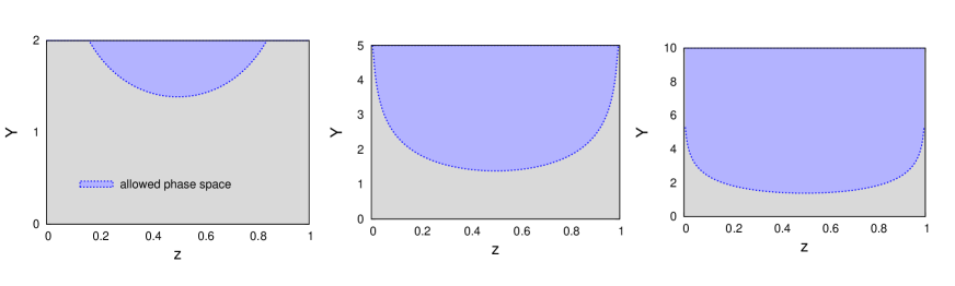
Figure 1: The range (6) of $z$-values, which are kinematically allowed in the evolution of the single-parton distributions $D_{q}(x,Y)$, $D_{g}(x,Y)$ up to $Y=2$ (left), $Y=5$ (middle), $Y=10$ (right).

One can check that if (6) is satisfied, then the arguments $\left(Y+\ln z\right)$ and $\left(Y+\ln(1-z)\,\right)$ of the functions $D_{q}$ and $D_{g}$ in (2) cannot be negative. The coupling constant can be written as

$$\alpha_{s}(k^{2}_{\perp})=\frac{\pi}{2N_{c}\,\beta}\,\frac{1}{Y+\ln z+\ln(1-z)+\lambda},\quad\beta=\frac{1}{4N_{c}}\left(\frac{11}{3}N_{c}-\frac{4}{3}n_{f}T_{R}\right),\quad\lambda=\ln\frac{Q_{0}}{\Lambda_{\rm QCD}}.$$ (7)

2.1 Initial conditions and ansatz for solution

A parton shower in the real world is pictured often as a quark or a gluon produced initially with high energy and virtuality and evolving perturbatively from large $Y$ to a small hadronic scale $Y_{0}$. Evolution occurs by emitting partons at smaller and smaller angles, till a minimal angle $\theta_{0}$ is reached, at which non-perturbative hadronic effects set in. The numerical solution of the evolution equations (2) will proceed in the opposite direction, that is, the initial conditions for the solution of (2) are set at the small scale $Y_{0}$ which corresponds to the final partonic state of the physical process. These initial conditions specify which partons are measured. For instance, consider the initial condition

$$D_{q}(x,Y_{0})=\delta(1-x)\,,\qquad D_{g}(x,Y_{0})=0\,.\qquad\hbox{(Case I)}$$ (8)

This initial condition for the evolution equation specifies that the partons at the low scale $Y_{0}$ cannot split further and, by virtue of the choice (8), these partons are quarks. Starting the evolution from the initial condition (8), the functions $D_{q}(x,Y)$ and $D_{g}(x,Y)$ denote the single-quark distributions in a quark and a gluon jet, respectively. Alternatively, for the initial condition

$$D_{q}(x,Y_{0})=0\,,\qquad D_{g}(x,Y_{0})=\delta(1-x)\,,\qquad\hbox{(Case II)}$$ (9)

the functions $D_{q}(x,Y)$ and $D_{g}(x,Y)$ denote the single-gluon distributions in a quark and a gluon jet, respectively. Previous studies [5, 7, 6, 8, 9, 10, 11, 12, 13] have focused on the distribution of all partons in a quark or a gluon jet. This is obtained by evolving $D_{q}(x,Y)$ and $D_{g}(x,Y)$ from the initial condition

$$D_{q}(x,Y_{0})=\delta(1-x)\,,\qquad D_{g}(x,Y_{0})=\delta(1-x)\,.\qquad\hbox{(Case III)}$$ (10)

In Sec. 3 of this paper we present the results for the case of the initial condition (III) whereas in Sec. 4 we consider cases (I) and (II).

The most general ansatz for the solutions of the evolution equations (2) reads

$$D_{q}(l,Y) = S_{q}(Y)\,\delta(l)+Q(l,Y),$$ (11)

$$D_{g}(l,Y) = S_{g}(Y)\,\delta(l)+G(l,Y).$$ (12)

Here, the discrete parts are expressed in terms of the Sudakov form factors $S_{q}(Y)$ and $S_{g}(Y)$, which denote the probability that a parton does not split in the evolution between $Y_{0}$ and $Y$. These discrete terms arise as a natural consequence of the initial conditions (8), (9) and (10). The continuous parts $Q(l,Y)$ and $G(l,Y)$ vanish at the initial scale $Y=Y_{0}$ and arise from the further evolution with (2).

2.2 The MLLA evolution equations

In the following sections, we shall compare the numerical solution of (2) to the results obtained in the MLLA approach. Here, we recall the main approximations involved in deriving MLLA from the Eqs. (2). For more details about MLLA, we refer to [5, 1].

In the limit of large $Y$ and small $x$ one can perform an expansion of Eqs. (2) in powers of $\sqrt{\alpha_{s}}$. Formally, this is done by treating logarithms $Y$ and $\ln 1/x$ as being of order $1/\sqrt{\alpha_{s}}$. Keeping only terms of order ${\cal O}(\sqrt{\alpha_{s}})$ on the right hand side of Eqs. (2) (i.e. keeping terms of order ${\cal O}(1)$ in the distributions $D_{q}$ and $D_{g}$), these equations reduce to the DLA evolution equations with running coupling. The subleading corrections to DLA are obtained by keeping terms up to ${\cal O}(\alpha_{s})$ on the right hand side of (2) (thus keeping terms of order ${\cal O}(\sqrt{\alpha_{s}})$ in $D_{q}$ and $D_{g}$). This leads to [19]

$$\partial_{Y}D_{q}(x,Y) = \frac{C_{F}}{N_{c}}\left\{\int^{1}_{0}\frac{dz}{z}\,\gamma_{0}^{2}(Y+\ln z)\,D_{g}\Big{(}\frac{x}{z},Y+\ln z\Big{)}-a_{qg}\,\gamma_{0}^{2}(Y)\,D_{g}\left(x,Y\right)\right\},\hskip 28.45274pt$$ (13)

$$\partial_{Y}D_{g}(x,Y) = \int^{1}_{0}\frac{dz}{z}\,\gamma_{0}^{2}(Y+\ln z)\,D_{g}\Big{(}\frac{x}{z},Y+\ln z\Big{)}-a_{gq}\,\gamma_{0}^{2}(Y)\,D_{q}\left(x,Y\right)-a_{gg}\,\gamma_{0}^{2}(Y)\,D_{g}\left(x,Y\right),$$

where $\gamma^{2}_{0}(Y)=1/(\beta(Y+\lambda))$ and

$$a_{qg}=\frac{3}{4},\qquad a_{gq}=-\frac{2}{3}\frac{n_{f}T_{R}}{N_{c}},\qquad a_{gg}=\frac{1}{4N_{c}}\left(\frac{11}{3}N_{c}+\frac{4}{3}n_{f}T_{R}\right).$$ (15)

In deriving Eqs. (13) and (2.2), the semi-hard splittings $z\sim 1$ from the evolution equation (2) have been taken into account only partially. For this reason, energy is not conserved exactly in the above equations.

Formally, to arrive at the MLLA equation [5, 1], one requires the DLA relation

$$D_{q}(l,Y)=\frac{C_{F}}{N_{c}}D_{g}(l,Y)\,.$$ (16)

By inserting this expression into (2.2), one obtains a closed equation for the parton distribution in a gluon jet

$$\partial_{Y}D_{g}(x,Y)=\int^{1}_{0}\frac{dz}{z}\,\gamma_{0}^{2}(Y+\ln z)\,D_{g}\Big{(}\frac{x}{z},Y+\ln z\Big{)}-a_{1}\,\gamma_{0}^{2}(Y)\,D_{g}\left(x,Y\right),$$ (17)

where

$$a_{1}=a_{gg}+\frac{C_{F}}{N_{c}}a_{gq}=\frac{1}{4N_{c}}\left[\frac{11}{3}N_{c}+\frac{4}{3}n_{f}T_{R}\left(1-\frac{2C_{F}}{N_{c}}\right)\right].$$ (18)

Eq. (17) is commonly referred to as MLLA evolution equation. From this, the parton distribution in a quark jet is usually determined with the help of (16). Compared to the DLA approximation, the MLLA equation shows mainly two improvements: the coupling constant is running and the negative term $\propto-\gamma_{0}^{2}(Y)G\left(x,Y\right)$ on the right hand side of Eq. (17) accounts for recoil effects which lead to a softening of the spectra as compared to DLA.

We note that the MLLA evolution equation (17) propagates only the initial conditions (II) or (III), which give the same result for $D_{g}(x,Y)$. This is because within the MLLA approach one cannot differentiate between quarks and gluons in a quark or a gluon jet. In the following, all numerical results for the MLLA evolution are obtained with the initial conditions $D_{g}(x,Y)=\delta(1-x)$. Using the ansatz (12) one obtains from Eq. (17) the MLLA Sudakov form factor

$$S_{\rm MLLA}(Y)=\left(\frac{Y+\lambda}{\lambda}\right)^{-a_{1}/\beta}\,$$ (19)

and the equation for the continuous part $G(l,Y)$.

2.3 Evolution equations in the coherent branching formalism

In this subsection, we return to the full evolution equations (2) of the coherent branching formalism. Inserting the ansatz (11), (12) into (2), we find for the Sudakov form factors

$$\partial_{Y}S_{q}(Y) = -\frac{1}{2}\int^{z_{+}}_{z_{-}}dz\,\frac{\alpha_{s}(k^{2}_{\perp})}{\pi}\,\left[P_{qq}(z)+P_{gq}(z)\right]S_{q}(Y),$$ (20)

$$\partial_{Y}S_{g}(Y) = -\frac{1}{2}\int^{z_{+}}_{z_{-}}dz\,\frac{\alpha_{s}(k^{2}_{\perp})}{\pi}\,\left[P_{gg}(z)+2n_{f}P_{qg}(z)\right]S_{g}(Y).$$ (21)

The above equations are not coupled and can be easily solved. It follows from the integration boundaries $z_{-}$, $z_{+}$ given in (6), that

$$S_{q}(Y)=S_{g}(Y)=1\qquad{\rm for}\ Y<\ln 4\,.$$ (22)

After exploiting the $z\leftrightarrow 1-z$ symmetry of the transverse momentum (5) and the integration boundaries, and with the help of the property $P_{qq}(z)=P_{gq}(1-z)$, we find for the initial condition (10) and for $Y>\ln 4$

$$S_{q}(Y) = \exp\left\{-\frac{C_{F}}{2N_{c}\beta}\int_{\ln 4}^{Y}dY^{\prime}\int^{z_{+}}_{z_{-}}\frac{dz}{Y^{\prime}+\ln z(1-z)+\lambda}\,\frac{1+z^{2}}{1-z}\right\},$$ (23)

$$S_{g}(Y) = \exp\Bigg{\{}-\frac{1}{4N_{c}\beta}\int_{\ln 4}^{Y}dY^{\prime}\int^{z_{+}}_{z_{-}}dz\,\frac{dz}{Y^{\prime}+\ln z(1-z)+\lambda}\,$$ (24)

$$\qquad\times\left[2C_{A}\left(\frac{1-z}{z}+\frac{z}{1-z}+z(1-z)\right)+2n_{f}T_{R}\left(z^{2}+(1-z)^{2}\right)\right]\Bigg{\}}.$$

We have performed the double integrals in Eqs. (23) and (24) numerically. Fig. 2 shows the result for three values of $\lambda$. For $Y>\ln 4$, these factors decrease almost exponentially in sharp contrast to the MLLA behavior (19). One can show that for large $Y$ the slope changes with $Y$ according to

$$\frac{d\ln S_{q,g}}{dY}\simeq-c_{q,g}\,\ln\left[\frac{Y+\lambda}{\lambda}\right],$$ (25)

where $c_{q}=C_{F}/(N_{c}\beta)$ and $c_{g}=1/\beta$.

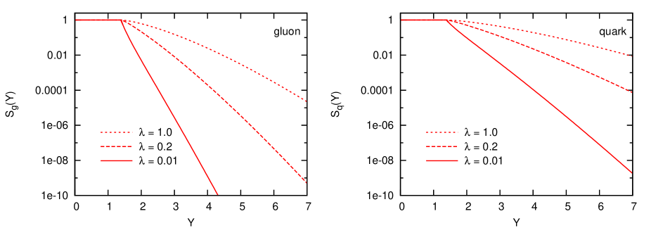
Figure 2: The Sudakov form factors (23) and (24) for three different values of $\lambda$.

The solutions $S_{q}(Y)$, $S_{g}(Y)$ enter the evolution equations for $Q(l,Y)$ and $G(l,Y)$. After changing the integration variable $z$ to $\bar{l}=\ln(z/x)$, the equations for the continuous parts of the spectra can be written as

$$\partial_{Y}Q(l,Y) = \int^{\bar{l}_{\rm max}}_{\bar{l}_{\rm min}}d\bar{l}\,\Gamma_{s}(l-\bar{l},Y)\,\bigg{\{}P_{qq}(l-\bar{l})\,Q(\bar{l},Y-l+\bar{l})+P_{gq}(l-\bar{l})\,G(\bar{l},Y-l+\bar{l})\bigg{\}}$$

$$\hskip 5.0pt+\ \Gamma_{s}(l,Y)\bigg{\{}P_{qq}(l)\,S_{q}(Y-l)+P_{gq}(l)\,S_{g}(Y-l)\bigg{\}}+\partial_{Y}\!\ln S_{q}(Y)\,Q(l,Y),$$

$$\partial_{Y}G(l,Y) = \int^{\bar{l}_{\rm max}}_{\bar{l}_{\rm min}}d\bar{l}\,\Gamma_{s}(l-\bar{l},Y)\,\bigg{\{}P_{gg}(l-\bar{l})\,G(\bar{l},Y-l+\bar{l})+2n_{f}P_{qg}(l-\bar{l})\,Q(\bar{l},Y-l+\bar{l})\bigg{\}}$$

$$\hskip 5.0pt+\ \Gamma_{s}(l,Y)\bigg{\{}P_{gg}(l)\,S_{g}(Y-l)+2n_{f}P_{qg}(l)\,S_{q}(Y-l)\bigg{\}}+\partial_{Y}\!\ln S_{g}(Y)\,G(l,Y),$$

where we have introduced the shorthand

$$\Gamma_{s}(l,Y)=\frac{1}{2N_{c}\beta}\,\frac{e^{-l}}{Y-l+\ln(1-e^{-l})+\lambda}.$$ (27)

The limits of integration in Eq. (2.3) are

$$\bar{l}_{\rm min}=l-\ln\frac{2}{1-\sqrt{1-4e^{-Y}}}\,,\qquad\bar{l}_{\rm max}=l-\ln\frac{2}{1+\sqrt{1-4e^{-Y}}}\,.$$ (28)

We recall that the functions $G(l,Y)$ and $Q(l,Y)$ vanish when the first argument is negative. We also note that the form (2.3) for the evolution equations in the coherent branching formalism is valid for all initial conditions and the logarithmic derivatives $\partial_{Y}\!\ln S_{q,g}(l,Y)$ on the right hand side of these evolution equations are formal notational shortcuts, denoting the expressions (23), (24) irrespective of the initial conditions. These logarithmic derivatives decrease only logarithmically with $Y$, as seen from Eq. (25). Hence, the rapid decrease of the Sudakov form factors itself does not render the corresponding terms in (2.3) negligible at large $Y$.

3 Numerical results

We have solved numerically the evolution equations for the continuous parts of single particle distributions in quark and gluon jets in the coherent parton branching formalism (2.3) and in the MLLA approach (17). The solutions depend on

$$\lambda=\ln Q_{0}/\Lambda_{\rm QCD}\,,$$ (29)

which specifies in units of $\Lambda_{\rm QCD}$ the value of the hadronization scale $Q_{0}$ up to which the parton shower is evolved. It is a peculiar feature of the MLLA approach, that its solutions have a well-defined finite limit $\lambda\to 0$, which is known as the “limiting spectrum” and which is at the basis of many phenomenological comparisons [1, 14, 15, 20, 21]. In general, however, one cannot expect to obtain finite results in the limit $\lambda\to 0$, since $\lambda$ regulates the Landau pole of the strong coupling constant (7). In fact, we shall find that the solutions for the evolution equations  (2) can be obtained for a finite value of $\lambda$, only.

In the following, we show numerical results for $\lambda=0.01$, $\lambda=0.2$ and $\lambda=1.0$. The MLLA limiting spectrum is approximately $3-4\%$ larger in norm and similar in shape, compared to the MLLA solution for $\lambda=0.01$. Hence, our choice for this smallest value of $\lambda$ is motivated by the interest in exploring the solutions of the coherent branching formalism  (2) for a parameter range in which the MLLA limiting spectrum is almost reached. Our choice of the largest value $\lambda=1.0$ is motivated by the fact that parton showers implemented in Monte Carlo event generators typically end the perturbative evolution at a hadronization scale $Q_{0}$ which is significantly larger than $\Lambda_{\rm QCD}$ and for which $\lambda\sim 1$ is an order of magnitude estimate. We have chosen one value $\lambda=0.2$ in between, and it is for this value that we shall first present our results.

3.1 The distributions $Q(l,Y)$ and $G(l,Y)$

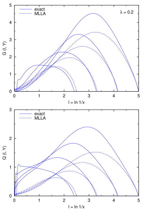
Figure 3: The continuous parts of the inclusive distribution of all partons in gluon (upper panel) and quark jet (lower panel). Results are shown for evolution in the coherent parton branching formalism (2), and in the MLLA approach (17) for $\lambda=0.2$ and $Y=$ 2.5, 3.3, 4.2 and 5.0.

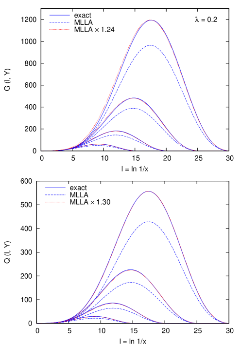
Figure 4: Same as Fig. 3, but for evolution up to $Y=15$, $20$, $25$ and $30$.

In Figs. 3 and  4, we present results for the continuous part of the single-parton distributions inside a quark and a gluon jet, evolved from the initial condition (10) at $Y_{0}=0$ up to different values of $Y$. Fig. 3 shows results for the evolution up to values of $Y\leq 5$ whereas Fig. 4 focuses on evolution to much larger values $15\leq Y\leq 30$. The relation between the evolution variable $Y$ and the jet energy $E$ depends on the jet opening angle $\theta$ and the hadronization scale $Q_{0}$, as seen from Eq. (1). In the case of large angles, the approximate formula (1) must be replaced by the exact relation $Y=\ln(E\sin\theta/Q_{0})$. For a given jet energy, the maximal value of $Y$ is obtained with the maximal choice for $\theta$ and the minimal choice for $Q_{0}$. For instance, for a maximal angle, $\theta=\pi/2$, and a very low value $Q_{0}=200$ MeV, the value of $Y=5$ corresponds to an energy of $E=30$ GeV and $Y=7$ corresponds to $E=220$ GeV. On the other hand, for a smaller opening $\theta=0.3$, a choice of $Y=5$ corresponds to $E=100$ GeV. Also, for $\theta=0.3$, $Y=5$ corresponds to $E=250$ GeV if one chooses a larger hadronization scale $Q_{0}=500$ MeV. These numerical examples illustrate that while the correspondence between jet energy and $Y$ may vary significantly depending on the choice of $Q_{0}$, the range of $Y\leq 5-7$ matches quite well the entire range of jet energies which have been compared so far to data on inclusive single hadronic distributions inside jets. This is one reason for considering first the evolution up to $Y=5$. We note that similar numerical estimates relate $Y=10$ to a minimal jet energy $E>4$ TeV. So, our choice of larger values of $Y$ can be motivated solely by the theoretical interest of testing the asymptotic behavior of these evolution equations. In addition, we recall that the evolution equations (2) have been derived in an approximation, in which logarithms are large and corrections of order $Y\sim 1/\sqrt{\alpha_{s}}$ are kept. Starting at $Y_{0}$, some evolution will be necessary to satisfy this condition. As we shall see, this initial stage of the evolution leads to some peculiar features in the solution which can persist up to values of $Y=5$ or larger.

We consider first the case for $Y<5$. As seen in Fig. 3, the single inclusive distributions obtained for the evolution within the coherent branching formalism show for small $Y$ a large yield at low values of $l\ll Y$. This effect is more pronounced for the distribution in a quark jet, than for the distribution in a gluon jet. It can be understood on general grounds from the fact that the initial conditions (10) for the evolution are delta-functions at $l=0$, and that the results for small $Y$ remember these initial conditions. Moreover, quarks are less likely to branch than gluons, and in their first branching they are likely to keep a large fraction of their energy. This tends to make the distribution in a quark jet harder than in a gluon jet, as clearly seen in Fig. 3. Upon further evolution to $Y=3.3,4.2,5.0$, the yield of hard partons (say partons with $l<1$) in a gluon jet decreases rapidly to a value comparable with (and for some region of $l$ even smaller than) the results obtained in the MLLA approach. On the other hand, the yield of hard partons in a quark jet remains enhanced significantly over the yield obtained in the MLLA approach up to relatively large values of the evolution parameter $Y$. We recall that the parametric reasoning underlying the evolution equations (2) is valid for sufficiently large $Y$ and $l\sim{\cal O}(Y)$. However, also in the region around the peak of the single inclusive distributions (which will lie for sufficiently large $Y$ within this kinematic range of validity), there are significant differences between the MLLA approach and the coherent branching formalism.

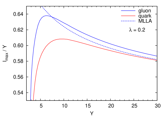
Figure 5: The evolution in $Y$ of the peak position of the continuous parts of the inclusive parton distributions. Results are shown for all partons in a gluon jet (upper straight line) or a quark jet (lower straight line), calculated in the coherent parton branching formalism (2). Results are also shown for the MLLA approach (17) (dashed line), for which the peak positions of the distributions for quark and gluon jets coincide. All results are calculated for $\lambda=0.2$ and the peak position $l_{\rm max}$ is plotted in units of $Y$.

From Fig. 3, we have seen several preasymptotic features, which become less pronounced upon further evolution in $Y$. Fig. 4 illustrates the degree to which these preasymptotic features disappear with increasing $Y$. The numerical results for the coherent branching formalism and the MLLA approach agree very well in shape and differ in norm by a factor of order unity which is $Y$-independent to good accuracy. Closer investigation shows that the factors needed to adjust the norm between both approaches differ for gluon jets (normalization factor 1.24 for $\lambda=0.2$) and quark jets (normalization factor 1.30 for $\lambda=0.2$). Fig. 4 illustrates the statement that in the asymptotic region of evolution towards sufficiently large $Y$, the region around the peak of the single-parton distributions lies at sufficiently large $l$ to be calculable within the accuracy of the single branching formalism. In this asymptotic region, MLLA and coherent branching formalism agree up to the norm. On the other hand, Fig. 3 illustrates that for $\lambda=0.2$, this asymptotic region is not yet reached for $Y\leq 5-7$, which is the range in which the bulk of the currently known experimental data lie.

To further illustrate the slow but steady convergence in shape between the MLLA results for single-parton distributions and those of the coherent branching formalism, we have plotted in Fig. 5 the evolution of the peak position of these distributions as a function of $Y$. We see that the peak positions in both approaches differ largely for $Y\leq 5-7$, consistent with our earlier remarks. In general, the gluon jets split more than quark jets and thus show a softer distribution and a peak at larger value of $l_{\rm max}$. This difference, however, decreases with increasing $Y$, as does the difference with the peak position in the MLLA approach. The value of $l_{\rm max}/Y$ decreases slowly with $Y$, but even for the largest values explored here (i.e. $Y=30$ corresponding to the jet energy of $E\sim 10^{12}$ GeV), the position of the peak differs significantly from the DLA result $l_{\rm max}/Y=1/2$.

3.2 Total multiplicity and energy conservation

The single-parton distributions inside quark and gluon jets can be characterized by their moments. The zeroth and first moments of the inclusive single-parton distributions are of particular interest, since they define the total parton multiplicity in a quark or gluon jet,

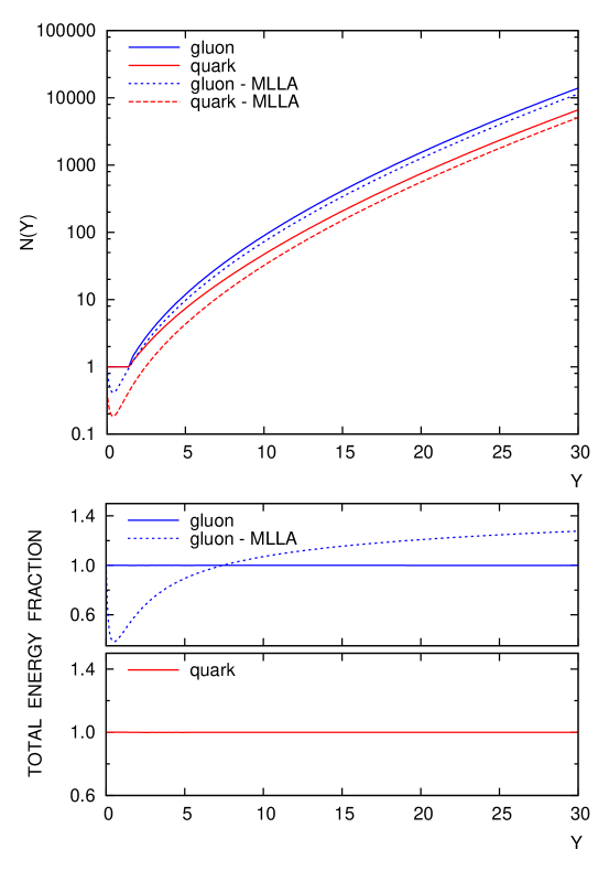
Figure 6: Upper plot: $Y$-dependence of the total parton multiplicity (30) in a quark or gluon jet, calculated in the coherent parton branching formalism (2) (straight lines), and in the MLLA approach (17) (dashed lines) for $\lambda=0.2$. Lower plot: The ratio (31) of the total jet energy contained in the single parton distribution to the initial jet energy. The upper panel is for gluon jets, the lower one for quark jets, $\lambda=0.2$.

$$N_{q,g}(Y)=\int\!\!dl\,D_{q,g}(l,Y)\,,$$ (30)

and the total energy fraction inside a quark or gluon jet

$$\frac{1}{E}\sum_{\rm partons}E_{p}(Y)=\int\!\!dx\,xD_{q,g}(x,Y)\,.$$ (31)

For an energy-conserving evolution of $D_{q,g}$, the first moment of the single-parton distribution must yield the total jet energy $E$, and the fraction (31) must equal one. The bottom panel of Fig. 6 illustrates, that this is satisfied for the coherent branching formalism. Since we know that the evolution equations (2) conserve energy, this is a cross check of the numerical accuracy of our solution. We note that the value of the first moment (31) is determined largely by $D_{q,g}(x,Y)$ in the region of large $x$. However, parametrically, the evolution equations (2) have been derived for the region of small $x$, where the logarithm $l$ is large. Fig. 6 also illustrates that the MLLA approach does not conserve energy exactly. So, on kinematic grounds, the coherent branching formalism is certainly preferable. We note, however, that for large values of $Y$, as seen in Fig. 4, the region around the peak of the distribution $D_{q,g}$ will be at $x$ values, which are much softer than the region of $x$ space which contributes dominantly to (31). For this reason, a formalism which does not conserve energy may account accurately for the functions $D_{q,g}(x,Y)$ in a wide region around the peak, if $Y$ is sufficiently large.

Within the MLLA approach, one customarily relates by a prefactor the single-parton distributions in quark and gluon jets, so that $G(x,Y)=N_{c}/C_{F}\>Q(x,Y)$. This relation is valid to DLA accuracy and leads to the first moment (31) of a quark jet equal to the total energy faction of a gluon jet multiplied by $4/9$. We did not include this result in Fig. 6, since it does not add further information.

We now turn to the total parton multiplicities within a quark or a gluon jet, plotted in the upper panel of Fig. 6. These multiplicities satisfy evolution equations for integrated parton distributions, which are much simpler than the set of equations (2), and which have been studied numerically [12, 13]. We checked that we reproduce these results, if we adopt the same modifications to the coherent branching formalism (2). We also tested the numerical accuracy of our routines for $D_{q,g}(x,Y)$, by comparing the integral (30) to the result of the simpler evolution equations for multiplicities, and we found perfect agreement. Within MLLA, the multiplicities for the limiting case ($\lambda=0$) and at large values of $Y$ are known to rise like [1, 2, 7]

$$N_{\rm MLLA}(Y)\sim Y^{-a_{1}/(2\beta)+1/4}\,e^{2\,\sqrt{Y/\beta}}\,.$$ (32)

This strong rise of the multiplicity is seen in Fig. 6. At large $Y$, the rise is the same in the MLLA approach and in the coherent branching formalism. In comparison to the MLLA approach, the multiplicities obtained in the coherent branching formalism are a factor $\sim 1.24$ for gluon jets and a factor $\sim 1.30$ higher for quark jets at large $Y$. This is consistent with our observation in Fig. 4 and indicates that at large $Y$, the distributions obtained in both approaches can be made to coincide by an approximately $Y$-independent multiplicative factor.

3.3 Dependence of $Q(x,Y)$ and $G(x,Y)$ on $\lambda$

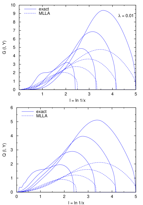
Figure 7: Same as Fig. 3 but for $\lambda=0.01$.

The numerical results shown in the previous subsections  3.1 and  3.2 were obtained for $\lambda=0.2$. Here, we discuss the dependence of these results on $\lambda$. From the point of view of data comparison, it is natural to regard the jet energy $E$ and the hadronization scale $Q_{0}$ as the two independent variables, while $\Lambda_{\rm QCD}$ is fixed. Specifying the $Y$-range of the evolution and the value of $\lambda$ amounts to specifying the variables $E$ and $Q_{0}$. On the other hand, regarding the values for the jet energy and the $Y$-range of the evolution as given, decreasing $\lambda$ amounts to increasing $\Lambda_{\rm QCD}$. As a consequence, a smaller value of $\lambda$ is expected to lead to a more ’violent’ evolution (i.e. more parton branchings) and it will thus lead to a higher jet multiplicity within the same $Y$-interval.

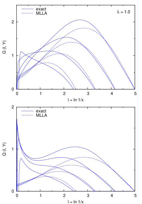
Figure 8: Same as Fig. 3 but for $\lambda=1.0$.

This general expectation is confirmed by the curves in Figs.  7 and 8, which show the distributions of all partons in a quark or a gluon jet for evolution over small $Y$-intervals up to $Y\leq 5$. In particular, one sees that after evolving for a few units in $Y$, the parton distributions for $\lambda=1.0$ are still peaked at very large values of $x$, where $\ln 1/x\ll 1$. Qualitatively, the structures at large $x$ are due to the fact, that for small $Y$ the phase space for evolution shown in Fig. 1 excludes evolution to very small values $x$, and the driving term of the evolution is the Sudakov form factor at $x=1$. Upon evolution in $Y$, this Sudakov form factor decreases faster for the more violent evolution with $\lambda=0.01$ than for less violent one with $\lambda=1.0$, as can be seen from Fig. 2. For this reason, the parton distributions in Fig. 7, which were calculated with $\lambda=0.01$, decrease under evolution in $Y$ much faster in the region of larger $x$, than distributions evolved with larger values of $\lambda$, shown in Figs. 3 and 8. The same qualitative features (though quantitatively less pronounced) are found in the MLLA approach, where for small $Y$ the continuous part of the single parton distribution differs significantly from zero at large $x$, in particular for the case $\lambda=1.0$ of a less violent evolution.

For $\lambda=0.01$ and $\lambda=1.0$, we have calculated the single-parton distributions inside quark and gluon jets for evolution up to $Y=30$ (results not shown). In this asymptotic regime, similarly to the case $\lambda=0.2$, the results obtained from the coherent branching formalism and the MLLA approach can be made to coincide by a simple adjustment of the norm. For $\lambda=1.0$, the MLLA results are at large values of $Y$ a factor 1.11 smaller for gluon jets and a factor 1.16 smaller for quark jets. For $\lambda=0.01$ the corresponding factors are 1.72 for gluon jets and 1.80 for quark jets. As noted before in studies of total jet multiplicities [12, 13], the coherent branching formalism does not allow for a limiting curve, $\lambda\to 0$, while the MLLA approach does. Our numerical findings are consistent with this observation and indicate that for decreasing $\lambda$, the difference in norm between both approaches increases slowly but without bound.

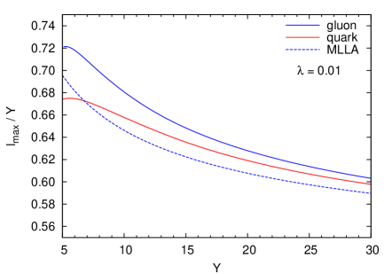
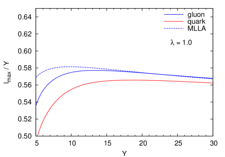
Figure 9: Same as Fig. 5 for $\lambda=0.01$ and $\lambda=1.0$.

For a more violent evolution, i.e. for smaller $\lambda$, single parton distributions increase in multiplicity and become softer. As a consequence, the peak position of the distributions is expected to shift to larger values of $\ln 1/x$ as $\lambda$ decreases. This expectation is confirmed in Fig. 9, which shows the peak positions of single-parton distributions for $\lambda=0.01$ and $\lambda=1.0$.

3.4 Matching MLLA to the coherent branching formalism

As shown in Figs. 3,  7 and  8, single parton distributions calculated in the MLLA approach differ for $Y\leq 5$ both in norm and in shape from those calculated in the coherent branching formalism. Besides the normalization, the spectra depend on two additional parameters, namely $Q_{0}$ and $\Lambda_{\rm QCD}$ or equivalently $Y$ and $\lambda$. Here we ask to what extent a variation of the three parameters is sufficient to make results from the coherent branching formalism coincide with a given result of the limiting fragmentation function ($\lambda\to 0$) obtained in the MLLA approach. One motivation for this study comes from the observation that the MLLA limiting fragmentation function is at the basis of many phenomenologically successful comparisons. So, even if the comparison of QCD predictions for single-hadron distributions in jets is not restricted to the calculation of single-parton distributions and involves difficult issues in the modeling of hadronization, one wonders to what extent the shape of partonic distributions in the two calculational schemes can be made to agree by a suitable choice of parameters.

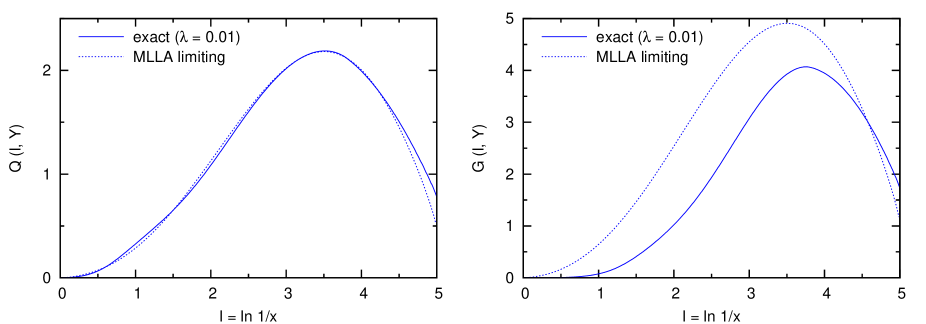
Figure 10: The continuous parts of single parton distributions. Dashed lines: the MLLA limiting fragmentation for $Y=5.0$. Solid lines: results for the coherent branching formalism with a choice of $\lambda=0.01$, $Y=5.2$ and norm adjusted to $0.405$ such that the distributions in quark jets almost match.

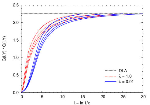
Figure 11: The ratio $G(l,Y)/Q(l,Y)$ in the coherent branching formalism for two different values of $\lambda$ and evolution up to different $Y=15$, $20$, $25$ and $30$, from top to bottom. By construction, MLLA results assume the DLA relation (16).

Fig. 10 shows an example of the extent to which this is possible. Adjusting the norm, the evolution time, $Y$, and the value of $\lambda$, the single-parton distributions in a quark jet can be made to coincide almost for both formalisms at $Y=5$. More generally, one sees from Figs. 5 and  9 that the peak position of the single-parton distributions in either a quark or a gluon jet can always be adjusted to agree between both approaches by varying $Y$ and $\lambda$ in the coherent branching formalism. The total yield can then be adjusted by the norm.

On the other hand, it is not possible for $Y\sim 5$ and with the same choice of $\lambda$ to get results of both formalisms to coincide for the distributions in both quark and gluon jets . This is illustrated by the example given in Fig. 10, where marked differences persist between the distributions in gluon jets, once the distributions in quark jets have been adjusted. This conclusion is supported more generally by Fig. 11, which shows the ratio of single-parton distributions of a gluon and a quark jet. Within the MLLA approach, these distributions vary in norm but not in shape, since the ratio $G(l,Y)/Q(l,Y)$ is fixed to the DLA value $N_{c}/C_{F}$. On the contrary, within the coherent branching formalism, the distributions in a quark jet and a gluon jet vary both in norm and shape. In this latter case, the deviation from $N_{c}/C_{F}$ is more pronounced in the region of relatively large $x$, and upon evolution in $Y$ this region becomes disentangled from the region around the peak of the distribution. In short, while there are marked differences between both formalisms at all $Y$, for sufficiently large $Y$ these differences die out in the region of large $l\sim{\cal O}(Y)$ to which the coherent branching formalism and the MLLA approach are tailored.

4 Identified parton distributions in quark and gluon jet

So far, we have discussed the distribution of all partons within a quark or a gluon jet. In the coherent branching formalism, we can study separately the distribution of quarks and gluons within a quark or a gluon jet. We characterize these distributions by subscripts. For instance, $Q^{g}(l,Y)$ is the single-gluon distribution in a quark jet. As explained in subsection 2.1, single-quark distributions are obtained by evolving from the initial conditions (8) and single-gluon distributions are obtained by evolving from the initial condition (9). The phase space constraints imply that there is no evolution in the coherent branching formalism up to $Y=\ln 4$. Since the continuous parts of the distributions vanish by definition at $Y=\ln 4$, the initial conditions (8) and (9) translate directly to the initial conditions for the Sudakov form factors

$$\begin{array}[]{lll}S_{g}(Y=\ln 4)=0\,,&S_{q}(Y=\ln 4)=1\,,&\qquad{\rm if\ only\ quarks\ are\ counted,}\\ S_{g}(Y=\ln 4)=1\,,&S_{q}(Y=\ln 4)=0\,,&\qquad{\rm if\ only\ gluons\ are\ counted.}\end{array}$$ (33)

It is straightforward to check that if a Sudakov factor equals zero at $\ln 4$, then it stays zero at any value of $Y$.

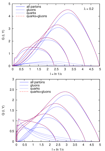
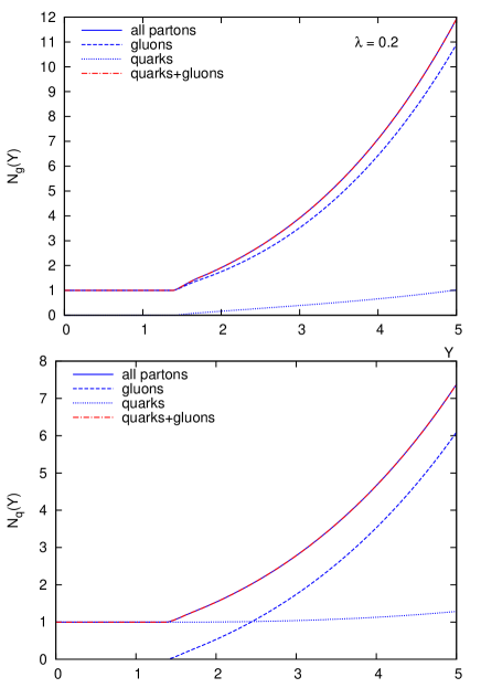
Figure 12: Left hand side: The continuous part of the single-parton distributions inside a gluon jet (upper panel) and a quark jet (lower panel). Different curves denote the single-quark (dashed) and single-gluon (dotted) distributions inside a jet, the explicit sum of these two distributions (dash-dotted), and its comparison to the distribution of all partons in a jet (solid) obtained by evolving the initial condition (10). The two latter curves coincide, as expected. Right hand side: the $Y$-dependence of the total multiplicity of quarks, gluons and all partons calculated for the cases shown on the left hand side.

In general, the distribution of quarks inside a jet is harder than that of gluons. This is a consequence of the fact that gluons are more likely to split. In the left panel of Fig. 12, which shows the identified parton spectra in jets for $\lambda=0.2$, this is clearly seen for all values of $Y$. A particularly pronounced feature is seen in the single-quark distribution for quark jets: up to $Y=5$, this distribution peaks at very large $x$ values corresponding to $l<0.5$. The integrated total quark multiplicity in this distribution, shown in the right panel of Fig. 12, grows slowly but remains of order unity during this evolution, indicating that this single quark distribution follows closely the momentum distribution of the evolved parent quark. This parent quark evolves via $q\to q\,g$ splittings predominantly by emitting soft gluons. For this reason, the quark distribution remains hard and the total multiplicity in the quark jet is largely dominated by subsequent $g\to g\,g$ splittings. It is in precisely this sense that the enhancement at large-$x$ is a remnant of the $\delta$-function in the initial condition, which gradually becomes negligible in the evolution to larger $Y$.

We have emphasized repeatedly that the approximations involved in deriving the coherent branching formalism do not guarantee an accurate description of the large-$x$ region. We note, however, that the reasons which we have identified for the pronounced large-$x$ enhancement of $Q^{q}(x,Y)$ in Fig. 12 do not refer to particular features of an ${\cal O}(\sqrt{\alpha_{s}})$ approximation, but emerge solely from generic features of the branching of quarks and gluons. As a consequence, we expect that these features, though observed outside the strict region of validity of the formalism explored here, correspond to physical reality and persist in a more complete formulation of the problem, which is accurate in the large-$x$ region. Indeed, in Monte Carlo event generators, such an enhancement is seen on the level of partonic distributions [16, 17, 18]. In these event generators, it is generally the hadronization mechanism which connects the color of the leading quark to the rest of the event, and which thus leads to a hadronic single-inclusive distribution which is much softer than the partonic one.

For the distribution of quarks within a gluon jet, the situation is clearly different since the splitting function for $g\to q\,\bar{q}$ does not give rise to a logarithmic enhancement. For this reason, the total quark multiplicity inside a quark or a gluon jet rises only slowly. For gluon jets as well as for quark jets, the jet multiplicity is ultimately dominated by gluons. The distribution of the hardest gluon in the first $g\to g\,g$ splitting process is likely to contribute significantly to the large values which $G(l,Y)$ shows in the large $x$ region (say $l<1.0$) for small values of $Y$. Upon further evolution in $Y$, this structure disappears faster in $G(l,Y)$ than in $Q(l,Y)$, since it is dominated in the first case by gluons, which split more readily than quarks.

5 Conclusion

We have calculated single parton distributions inside quark and gluon jets by solving the full evolution equations in the coherent branching formalism. For sufficiently large jet energies, corresponding to $Y>5-10$, results obtained from the MLLA and from the coherent branching formalism agree very well in shape. They differ in this asymptotic regime solely by a factor of order unity in norm, and this factor depends weakly on the choice of hadronization scale. For smaller values of the jet energy ($Y\leq 5-7$), however, both formalisms show marked differences in norm and shape. We have characterized these differences in detail in sections 3 and  4.

We recall that, parametrically, both MLLA and the coherent branching formalism are valid for sufficiently large $Y$ in a kinematic region in which $l\sim{\cal O}(Y)$. As a consequence, the differences observed between both approaches for $Y\leq 5-7$ can be regarded as preasymptotic effects, which persist solely outside the strict region of validity of both approaches. If one adopts this view, then our study has contributed to delineating the region of quantitatively reliable applicability of both approaches, namely $Y>5-7$. In this context, we note that for $Y<5-7$, single-parton distributions in both approaches cannot be made to coincide by a suitable choice of parameters for both quark and gluon jets, while they can be made to coincide for one of them, see section 3.4.

On the other hand, the MLLA limiting spectrum has been compared successfully to a large data set of single inclusive hadronic distributions for jet energies, which lie in the range $Y\leq 5-7$. These data comparisons required the assumption of local parton hadron duality and, by their success, gave support to this assumption. In the present work, we have found that for $Y\leq 5-7$, distributions calculated in the coherent branching formalism show a significant enhancement at large $x$, which is much less pronounced and vanishes much faster with $Y$ in the MLLA approach. Also, this enhancement has not been observed in the measured hadronic distributions.

Although these findings were made in the region of small $Y$ and large $x$, which lies clearly outside the region of quantitative applicability of the formalisms in question, we have argued in section 4 that the structures found at large $x$ in the coherent branching formalism emerge solely from generic properties of the branching of quarks and gluons and should thus persist in a more complete formulation of the problem, which is reliable at small $Y$ and large $x$. We note that the marked difference between the shape of partonic distributions calculated in the coherent branching formalism and the shape of the measured hadronic distributions does not necessarily invalidate the coherent branching formalism in the range of $Y\sim 3-7$. Rather, this difference may be indicative of a non-trivial dynamics of hadronization, which is characteristically different from a simple one-to-one mapping of partons into hadrons at the scale $Q_{0}\sim{\cal O}(\Lambda_{\rm QCD})$. Indeed, since the hardest partonic components in a jet are connected to the softer ones by color flow, and since hadronization is ultimately sensitive to the color structure of the event, the dynamics of hadronization may lead to a significant softening of the single inclusive partonic large-$x$ distributions. Such features are realized at least in some models of hadronization, such as the Lund string model. If one adopts this view, then our study may be regarded as a contribution to the question to what extent the measured inclusive hadronic distributions inside jets lend support to a specific picture of hadronization.

References

- [1] Yu. L. Dokshitzer, V.A. Khoze, A. H. Mueller, S. I. Troyan, “Basics of Perturbative QCD”, Editions Frontierés, Gif-sur-Yvette (1991)
- [2] A. H. Mueller, Nucl. Phys. B 213 (1983) 85.
- [3] A. H. Mueller, Nucl. Phys. B 241 (1984) 141.
- [4] A. Bassetto, M. Ciafaloni and G. Marchesini, Phys. Rept. 100 (1983) 201.
- [5] Y. L. Dokshitzer, V. A. Khoze, S. I. Troian and A. H. Mueller, Rev. Mod. Phys. 60 (1988) 373.
- [6] C. P. Fong and B. R. Webber, Nucl. Phys. B 355, 54 (1991).
- [7] I. M. Dremin and V. A. Nechitailo, Mod. Phys. Lett. A 9 (1994) 1471 [arXiv:hep-ex/9406002].
- [8] F. Arleo, R. P. Ramos and B. Machet, Phys. Rev. Lett. 100 (2008) 052002. [arXiv:0707.3391 [hep-ph]].
- [9] R. Perez-Ramos, F. Arleo and B. Machet, Phys. Rev. D 78 (2008) 014019 [arXiv:0712.2212 [hep-ph]].
- [10] I. M. Dremin and J. W. Gary, Phys. Lett. B459, 341 (1999).
- [11] A. Capella, I. M. Dremin, J. W. Gary, V. A. Nechitailo and J. Tran Thanh Van, Phys. Rev. D61, 074009 (2000).
- [12] S. Lupia and W. Ochs, Phys. Lett. B 418 (1998) 214 [arXiv:hep-ph/9707393].
- [13] S. Lupia and W. Ochs, Nucl. Phys. Proc. Suppl. 64 (1998) 74 [arXiv:hep-ph/9709246].
- [14] Y. I. Azimov, Y. L. Dokshitzer, V. A. Khoze and S. I. Troyan, Z. Phys. C 27 (1985) 65.
- [15] Y. I. Azimov, Y. L. Dokshitzer, V. A. Khoze and S. I. Troyan, Z. Phys. C 31 (1986) 213.
- [16] T. Sjostrand, S. Mrenna and P. Skands, JHEP 0605 (2006) 026 [arXiv:hep-ph/0603175].
- [17] G. Marchesini, B. R. Webber, G. Abbiendi, I. G. Knowles, M. H. Seymour and L. Stanco, Comput. Phys. Commun. 67 (1992) 465.
- [18] T. Gleisberg, S. Hoche, F. Krauss, A. Schalicke, S. Schumann and J. C. Winter, JHEP 0402 (2004) 056 [arXiv:hep-ph/0311263].
- [19] R. P. Ramos, JHEP 0606 (2006) 019. [arXiv:hep-ph/0605083].
- [20] M. Z. Akrawy et al. [OPAL Collaboration], Phys. Lett. B 247 (1990) 617.
- [21] D. E. Acosta et al. [CDF Collaboration], Phys. Rev. D 68 (2003) 012003.