The theory of magnetic field induced domain-wall propagation in magnetic nanowires

Abstract

A global picture of magnetic domain wall (DW) propagation in a nanowire driven by a magnetic field is obtained: A static DW cannot exist in a homogeneous magnetic nanowire when an external magnetic field is applied. Thus, a DW must vary with time under a static magnetic field. A moving DW must dissipate energy due to the Gilbert damping. As a result, the wire has to release its Zeeman energy through the DW propagation along the field direction. The DW propagation speed is proportional to the energy dissipation rate that is determined by the DW structure. An oscillatory DW motion, either the precession around the wire axis or the breath of DW width, should lead to the speed oscillation.

Magnetic domain-wall (DW) propagation in a nanowire due to a magnetic fieldOno ; Cowburn ; Erskine ; Parkin1 ; Erskine1 reveals many interesting behaviors of magnetization dynamics. For a tail-to-tail (TT) DW or a head-to-head (HH) DW (shown in Fig. 1) in a nanowire with its easy-axis along the wire axis, the DW will propagate in the wire under an external magnetic field parallel to the wire axis. The propagation speed $v$ of the DW depends on the field strengthErskine ; Parkin1 . There exists a so-called Walker’s breakdown field $H_{W}$Walker . $v$ is proportional to the external field $H$ for $H<H_{W}$ and $H\gg H_{W}$. The linear regimes are characterized by the DW mobility $\mu\equiv v/H$. Experiments showed that $v$ is sensitive to both DW structures and wire widthOno ; Cowburn ; Erskine . DW velocity $v$ decreases as the field increases between the two linear H-dependent regimes, leading to the so-called negative differential mobility phenomenon. For $H\gg H_{W}$, the DW velocity, whose time-average is linear in $H$, oscillates in fact with time Walker ; Erskine .

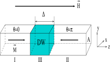
Figure 1: Schematic diagram of a HH DW of width $\Delta$ in a magnetic nanowire of cross-section $A$. The wire consists of three phases, two domains and one DW. The magnetization in domains I and II is along +z-direction ($\theta=0$) and -z-direction ($\theta=\pi$), respectively. III is the DW region whose magnetization structure could be very complicate. $\vec{H}$ is an external field along +z-direction.

It has been known for more than fifty years that the magnetization dynamics is govern by the Landau-Lifshitz-Gilbert (LLG)gilbert equation that is nonlinear and can only be solved analytically for some special problemsWalker ; xrw . The field induced domain-wall (DW) propagation in a strictly one-dimensional wire has also been known for more than thirty yearsWalker , but its experimental realization in nanowires was only achievedOno ; Cowburn ; Erskine ; Parkin1 ; Erskine1 in recent years when we are capable of fabricating various nano structures. Although much progressSlon ; Thiv has been made in understanding field-induced DW motion, it is still a formidable task to evaluate the DW propagation speed in a realistic magnetic nanowire even when the DW structure is obtained from various means like OOMMF simulator and/or other numerical software packages. A global picture about why and how a DW propagates in a magnetic nanowire is still lacking.

In this report, we present a theory that reveals the origin of DW propagation. Firstly, we shall show that no static HH (TT) DW is allowed in a homogeneous nanowire in the presence of an external magnetic field. Secondly, energy conservation requires that the dissipated energy must come from the energy decrease of the wire. Thus, the origin of DW propagation is as follows. A HH (TT) DW must move under an external field along the wire. The moving DW must dissipate energy because of various damping mechanisms. The energy loss should be supplied by the Zeeman energy released from the DW propagation. This consideration leads to a general relationship between DW propagation speed and the DW structure. It is clear that DW speed is proportional to the energy dissipation rate, and one needs to find a way to enhance the energy dissipation in order to increase the propagation speed. Furthermore, the present theory attributes a DW velocity oscillation for $H\gg H_{W}$ to the periodic motion of the DW, either the precession of the DW or oscillation of the DW width.

In a magnetic material, magnetic domains are formed in order to minimize the stray field energy. A DW that separates two domains is defined by the balance between the exchange energy and the magnetic anisotropy energy. The stray field plays little role in a DW structure. To describe a HH DW in a magnetic nanowire, let us consider a wire with its easy-axis along the wire axis (the shape anisotropy dominates other magnetic anisotropies and makes the easy-axis along the wire when the wire is small enough) which is chosen as the z-axis as illustrated in Fig. 1. Since the magnitude of the magnetization $\vec{M}$ does not change in the LLG equationxrw , the magnetic state of the wire can be conveniently described by the polar angle $\theta(\vec{x},t)$ (angle between $\vec{M}$ and the z-axis) and the azimuthal angle $\phi(\vec{x},t)$. The magnetization energy is mainly from the exchange energy and the magnetic anisotropy because the stray field energy is negligible in this case. The wire energy can be written in general as

$$\begin{split}&E=\int F(\theta,\phi,\vec{\nabla}\theta,\vec{\nabla}\phi)d^{3}\vec{x},\\ &F=f(\theta,\phi)+\frac{J}{2}[(\vec{\nabla}\theta)^{2}+\sin^{2}\theta(\vec{\nabla}\phi)^{2}]-MH\cos\theta,\end{split}$$ (1)

where $f$ is the energy density due to all kinds of magnetic anisotropies which has two equal minima at $\theta=0$ and $\pi$ ($f(\theta=0,\phi)=f(\theta=\pi,\phi)$), $J-$term is the exchange energy, $M$ is the magnitude of magnetization, and $H$ is the external magnetic field along z-axis. In the absence of $H$, a HH static DW that separates $\theta=0$ domain and $\theta=\pi$ domain (Fig. 1) can exist in the wire.

Non-existence of a static HH (TT) DW in a magnetic field-In order to show that no intrinsic static HH DW is allowed in the presence of an external field ($H\neq 0$), one only needs to show that following equations have no solution with $\theta=0$ at far left and $\theta=\pi$ at far right,

$$\begin{split}&\frac{\delta E}{\delta\theta}=J\nabla^{2}\theta-\frac{\partial f}{\partial\theta}-HM\sin\theta-J\sin\theta\cos\theta(\vec{\nabla}\phi)^{2}=0,\\ &\frac{\delta E}{\delta\phi}=J\vec{\nabla}\cdot(\sin^{2}\theta\vec{\nabla}\phi)-\frac{\partial f}{\partial\phi}=0.\end{split}$$ (2)

Multiply the first equation by $\nabla\theta$ and the second equation by $\nabla\phi$, then add up the two equations. One can show a tensor T satisfying $\nabla\cdot\hbox{\bf T}=0$ with

$$\hbox{\bf T}= [f-HM\cos\theta+\frac{J}{2}(|\nabla\theta|^{2}+\sin^{2}\theta|\nabla\phi|^{2})]\hbox{\bf 1}-$$

$$J(\nabla\theta\nabla\theta+\sin^{2}\theta\nabla\phi\nabla\phi),$$

where 1 is $3\times 3$ unit matrix. A dyadic product ($\nabla\theta\nabla\theta$ and $\nabla\phi\nabla\phi$) between the gradient vectors is assumed in T. If a HH DW exists with $\theta=0$ in the far left and $\theta=\pi$ in the far right, then it requires $-f(0,\phi)+HM=-f(\pi,\phi)-HM$ that holds only for $H=0$ since $f(0,\phi)=f(\pi,\phi)$. In other words, a DW in a nanowire under an external field must be time dependent that could be either a local motion or a propagation along the wire. It should be clear that the above argument is only true for a HH DW in a homogeneous wire, but not valid with defect pinning that changes Eq. (2). Static DWs exist in fact in the presence of a weak field in reality because of pinning.

What is the consequence of the non-existence of a static DW? Generally speaking, a physical system under a constant driving force will first try a fixed point solutionxrw2 . It goes to other types of more complicated solutions if a fixed point solution is not possible. It means that a DW has to move when an external magnetic field is applied to the DW along the nanowire as shown in Fig. 1. It is well knownThiv that a moving magnetization must dissipate its energy to its environments with a rate, $\frac{dE}{dt}=\frac{\alpha M}{\gamma}\int_{-\infty}^{+\infty}\left(d\vec{m}/dt\right)^{2}d^{3}\vec{x},$ where $\vec{m}$ is the unit vector of $\vec{M}$, $\alpha$ and $\gamma$ are the Gilbert damping constant and gyromagnetic ratio, respectively. Following the similar method in Reference 12 for a Stoner particle, one can also show that the energy dissipation rate of a DW is related to the DW structure as

$$\frac{dE}{dt}=-\frac{\alpha\gamma}{(1+\alpha^{2})M}\int_{-\infty}^{+\infty}\left(\vec{M}\times\vec{H}_{eff}\right)^{2}d^{3}\vec{x},$$ (3)

where $\vec{H}_{eff}=-\frac{\delta F}{\delta\vec{M}}$ is the effective field. In regions I and II or inside a static DW, $\vec{M}$ is parallel to $\vec{H}_{eff}$. Thus no energy dissipation is possible there. The energy dissipation can only occur in the DW region when $\vec{M}$ is not parallel to $\vec{H}_{eff}$.

DW propagation and energy dissipation-For a magnetic nanowire in a static magnetic field, the dissipated energy must come from the magnetic energy released from the DW propagation. The total energy of the wire equals the sum of the energies of regions I, II, and III (Fig. 1), $E=E_{I}+E_{II}+E_{III}$. $E_{I}$ increases while $E_{II}$ decreases when the DW propagates from left to the right along the wire. The net energy change of region I plus II due to the DW propagation is

$$\frac{d(E_{I}+E_{II})}{dt}=-2HMvA,$$ (4)

where $v$ is the DW propagating speed, and $A$ is the cross section of the wire. This is the released Zeeman energy stored in the wire. The energy of region III should not change much because the DW width $\Delta$ is defined by the balance of exchange energy and magnetic anisotropy, and is usually order of $10\sim 100nm$. A DW cannot absorb or release too much energy, and can at most adjust temporarily energy dissipation rate. In other words, $\frac{dE_{III}}{dt}$ is either zero or fluctuates between positive and negative values with zero time-average. Since energy release from the magnetic wire should be equal to the energy dissipated (to the environment), one has

$$-2HMvA+\frac{dE_{III}}{dt}=-\frac{\alpha\gamma}{(1+\alpha^{2})M}\int_{III}\left(\vec{M}\times\vec{H}_{eff}\right)^{2}d^{3}\vec{x}.$$ (5)

or

$$v=\frac{\alpha\gamma}{2(1+\alpha^{2})HA}\int_{III}\left(\vec{m}\times\vec{H}_{eff}\right)^{2}d^{3}\vec{x}+\frac{1}{2HMA}\frac{dE_{III}}{dt}.$$ (6)

Velocity oscillation-Eq. (6) is our central result that relates the DW velocity to the DW structure. Obviously, the right side of this equation is fully determined by the DW structure. A DW can have two possible types of motion under an external magnetic field. One is that a DW behaves like a rigid body propagating along the wire. This case occurs often at small field, and it is the basic assumption in Slonczewski modelSlon and Walker’s solution for $H<H_{W}$. Obviously, both energy-dissipation and DW energy is time-independent, $\frac{dE_{III}}{dt}=0$. Thus,and the DW velocity should be a constant. The other case is that the DW structure varies with time. For example, the DW may precess around the wire axis and/or the DW width may breathe periodically. One should expect both $\frac{dE_{III}}{dt}$ and energy dissipation rate oscillate with time. According to Eq. (6), DW velocity will also oscillate. DW velocity should oscillate periodically if only one type of DW motion (precession or DW breathing) presents, but it could be very irregular if both motions are present and the ratio of their periods is irrational. Indeed, this oscillation was observed in a recent experimentErskine . How can one understand the wire-width dependence of the DW velocity? According to Eq. (6), the velocity is a functional of DW structure which is very sensitive to the wire width. For a very narrow wire, only transverse DW is possible while a vortex DW is preferred for a wide wire (large than DW width). Different vortexes yield different values of $|\vec{m}\times\vec{H}_{eff}|$, which in turn results in different DW propagation speed.

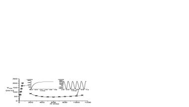
Figure 2: The time-averaged DW propagation speed versus the applied magnetic field for a biaxial magnetic nanowire of cross section $4nm\times 20nm$. The wire parameters are $K_{1}=K_{2}=10^{5}J/m^{3}$, $J=4.\times 10^{-11}J/m$, $M=10^{6}A/m$, and $\alpha=0.1$. Cross are for the calculated velocities from Eq. (7), and the open circles are for the simulated average velocities. The dashed straight line is the fit to the small $H<H_{W}$ results, and solid curve is the fit to $a(H-H_{0})^{2}/H+b/H$. Insets: the instantaneous DW speed calculated from Eq. (6) for $H=50Oe<H_{W}$ (left) and $H=1000Oe>H_{W}$ (right).

Time averaged velocity is

$$\bar{v}=\frac{\alpha\gamma}{2(1+\alpha^{2})HA}\int_{III}\overline{\left({\vec{m}\times\vec{H}_{eff}}\right)^{2}}d^{3}\vec{x},$$ (7)

where bar denotes time average. It says that the averaged velocity is proportional to the energy dissipation rate. In order to show that both Eqs. (6) and (7) are useful in evaluating the DW propagation speed from a DW structure. We use OOMMF package to find the DW structures and then use Eq. (7) to obtain the average velocity. Figure 2 is the comparison of such calculated velocities (cross) and numerical simulation (open circles with their error bars smaller than the symbol sizes) for a magnetic nanowire of cross-section dimension $4nm\times 20nm$ with a biaxial magnetic anisotropy $f=-\frac{K_{1}}{2}M_{z}^{2}+\frac{K_{2}}{2}M_{x}^{2}$. The system parameters are $K_{1}=K_{2}=10^{5}J/m^{3}$, $J=4.\times 10^{-11}J/m$, $M=10^{6}A/m$, and $\alpha=0.1$. The good overlap between the cross and open circles confirm the correctness of Eq. (7). The $\bar{v}-H$ curve for $H>H_{W}$ can be fit well by $a\Delta(H-H_{0})^{2}/H+b/H$ (see discussion later). The insets are instantaneous DW propagation velocities for both $H<H_{W}$ and $H>H_{W}$, by Eq. (6) from the instantaneous DW structures obtained from OOMMF. The left inset is the instantaneous DW speed at $H=50Oe<H_{W}$, reaching its steady value in about $1ns$. The right inset is the instantaneous DW speed at $H=1000Oe>H_{W}$, showing clearly an oscillation. They confirm that the theory is capable of capturing all the features of DW propagation.

The right side of Eq. (7) is positive and non-zero since a time dependent DW requires $\vec{m}\times\vec{H}_{eff}\neq 0$, implying a zero intrinsic critical field for DW propagation. If the DW keep its static structure, then the first term in the right side of Eq. (6) shall be proportional to $a\Delta AH^{2}$, where $a$ is a numerical number of order of 1 that depends on material parameters and the DW structure. This is because the effective field due to the exchange energy and magnetic anisotropy is parallel to $\vec{M}$, and does not contribute to the energy dissipation. Thus, in this case, $v=a\frac{\alpha\gamma\Delta}{1+\alpha^{2}}H$ with $\mu=a\frac{\alpha\gamma\Delta}{1+\alpha^{2}}$. Consider the Walker’s 1D modelWalker in which $f=-\frac{K_{1}}{2}M^{2}\cos^{2}\theta+\frac{K_{2}}{2}M^{2}\sin^{2}\theta\cos^{2}\phi,$ here $K_{1}$ and $K_{2}$ describe the easy and hard axes, respectively. From Walker’s trial function of a DW of width $\Delta$, $\ln\tan\frac{\theta(z,t)}{2}=\frac{1}{\Delta(t)}\left[z-\int_{0}^{t}v(\tau)d\tau\right]$ and $\phi(z,t)=\phi(t),$ one has (from Eq. (3)) the energy dissipation rate

$$\frac{dE}{dt}=-\frac{2\alpha\gamma A\Delta}{1+\alpha^{2}}\left[K_{2}^{2}M^{3}\sin^{2}\phi\cos^{2}\phi+H^{2}M\right],$$ (8)

and DW energy change rate is

$$\frac{dE_{III}}{dt}=\frac{d}{dt}\int_{III}F(\theta,\phi,\vec{\nabla}\theta,\vec{\nabla}\phi)d^{3}\vec{x}=-4JA\cdot\frac{\dot{\Delta}}{\Delta^{2}}.$$ (9)

Substituting Eqs. (8) and (9) into Eq. (6), one can easily reproduce Walker’s DW velocity expression for both $H<H_{W}$ and $\gg H_{W}$. For example, for $H<H_{W}=\alpha K_{2}M/2$ and $\Delta=const.$, Eq. (6) gives

$$v=\frac{\alpha\Delta\gamma}{1+\alpha^{2}}\left[1+\left(\frac{K_{2}M\sin\phi\cos\phi}{H}\right)^{2}\right]H.$$ (10)

This velocity expression is the same as that of the Slonczewski modelSlon for a one-dimensional wire. In Walker’s analysis, $\phi$ is fixed by $K_{2}$ and $H$ through $K_{2}M\sin\phi\cos\phi=\frac{H}{\alpha}$. Using this $\phi$ in the above velocity expression, Walker’s mobility coefficient $\mu=\frac{\gamma\Delta}{\alpha}$ is recovered. This inverse damping relation is from the particular potential landscape in $\phi$-direction. One should expect different result if the shape of the potential landscape is changed. Thus, this expression should not be used to extract the damping constantOno ; Erskine .

A DW may precess around the wire axis as well as be substantially distorted from its static structure when $H>H_{W}$ as it was revealed in Walker’s analysis. According to the minimum energy dissipation principleMea , a DW will arrange itself as much as possible to satisfy Eq. (2). Thus, the distortion is expected to absorb part of $H$. The precession motion shall induce an effective field $g(\phi)$ in the transverse direction, where $g$ depends on the magnetic anisotropy in the transverse direction. One may expect $\vec{m}\times\vec{H}_{eff}\simeq(H-H_{0})\sin\theta\hat{z}+\sin\theta g(\phi)\hat{y}$, where $H_{0}$ is the DW distortion absorbed part of $H$. Using $|\vec{m}\times\vec{H}_{eff}|^{2}=(H-H_{0})^{2}\sin^{2}\theta+g^{2}\sin^{2}\theta$ in Eq. (7), the DW propagating speed takes the following h-dependence, $v=a\alpha\gamma\Delta(H-H_{0})^{2}/H(1+\alpha^{2})+b\alpha\gamma\Delta/[H(1+\alpha^{2})]$, linear in both $\Delta$ and $H$ for $H\gg H_{0}$, but a smaller DW mobility. This field-dependence is supported by the excellent fit in Fig. 2 for $H>H_{W}$. The reasoning agrees also with the minimum energy dissipation principleMea since $|\vec{m}\times H_{eff}|=H\sin\theta$ when $\vec{M}$ for $H=0$ is used, and any modification of $\vec{M}$ should only make $|\vec{m}\times H_{eff}|$ smaller. The smaller mobility at $H\gg H_{W},H_{0}$ leads naturally to a negative differential mobility between $H<H_{W}$ and $H\gg H_{W}$! In other words, the negative differential mobility is due to the transition of the DW from a high energy dissipation structure to a lower one. This picture tells us that one should try to make a DW capable of dissipating as much energy as possible if one wants to achieve a high DW velocity. This is very different from what people would believe from Walker’s special mobility formula of inverse proportion of the damping constant. To increase the energy dissipation, one may try to reduce defects and surface roughness. The reason is, by minimum energy dissipation principle, that defects are extra freedoms to lower $|\vec{m}\times\vec{H}_{eff}|$ because, in the worst case, defects will not change $|\vec{m}\times\vec{H}_{eff}|$ when $\vec{M}$ without defects are used.

The correctness of our central result Eq. (6) depends only on the LLG equation, the general energy expression of Eq. (1), and the fact that a static magnetic field can be neither an energy source nor an energy sink of a system. It does not depend on the details of a DW structure as long as the DW propagation is induced by a static magnetic field. In this sense, our result is very general and robust, and it is applicable to an arbitrary magnetic wire. However, it cannot be applied to a time-dependent field or the current-induced DW propagation, at least not directly. Also, it may be interesting to emphasize that there is no inertial in the DW motion within LLG description since this equation contains only the first order time derivative. Thus, there is no concept of mass in this formulation.

In conclusion, a global view of the field-induced DW propagation is provided, and the importance of energy dissipation in the DW propagation is revealed. A general relationship between the DW velocity and the DW structure is obtained. The result says: no damping, no DW propagation along a magnetic wire. It is shown that the intrinsic critical field for a HH DW is zero. This zero intrinsic critical field is related to the absence of a static HH or a TT DW in a magnetic field parallel to the nanowire. Thus, a non-zero critical field can only come from the pinning of defects or surface roughness. The observed negative differential mobility is due to the transition of a DW from a high energy dissipation structure to a low energy dissipation structure. Furthermore, the DW velocity oscillation is attributed to either the DW precession around wire axis or from the DW width oscillation.

This work is supported by Hong Kong UGC/CERG grants (# 603007 and SBI07/08.SC09).

References

- (1) T. Ono, H. Miyajima, K. Shigeto, K. Mibu, N. Hosoito, and T. Shinjo, Science 284, 468 (1999).
- (2) D. Atkinson, D.A. Allwood, G. Xiong, M.D. Cooke, C. Faulkner, and R.P. Cowburn, Nat. Mater. 2, 85 (2003).
- (3) G.S.D. Beach, C. Nistor, C. Knutson, M. Tsoi, and J.L. Erskine, Nat. Mater. 4, 741 (2005); J. Yang, C. Nistor, G.S.D. Beach, and J.L. Erskine, Phys. Rev. B 77, 014413 (2008).
- (4) M. Hayashi, L. Thomas, Y.B. Bazaliy, C. Rettner, R. Moriya, X. Jiang, and S.S.P. Parkin, Phys. Rev. Lett. 96, 197207 (2006).
- (5) G.S.D. Beach, C. Knutson, C. Nistor, M. Tsoi, and J.L. Erskine, Phys. Rev. Lett. 97, 057203 (2006).
- (6) N.L. Schryer and L.R. Walker, J. of Appl. Physics, 45, 5406 (1974).
- (7) T. L. Gilbert, Phys. Rev. 100, 1243 (1955).
- (8) Z.Z. Sun and X.R. Wang, Phys. Rev. Lett. 97, 077205 (2006); X.R. Wang and Z.Z. Sun, ibid 98, 077201 (2007).
- (9) A.P. Malozemoff and J.C. Slonczewski, Magnetic Domain Walls in Bubble Material (Academica, New York, 1979).
- (10) A. Thiaville and Y. Nakatani in Spin Dynamics in Confined Magnetic Structures III Eds. B. Hillebrands and A. Thiaville, Springer 2002.
- (11) X. R. Wang, and Q. Niu, Phys. Rev. B 59, R12755 (1999); Z.Z. Sun, H.T. He, J.N. Wang, S.D. Wang, and X.R. Wang, Phys. Rev. B 69, 045315 (2004).
- (12) Z.Z. Sun, and X.R. Wang, Phys. Rev. B 71, 174430 (2005); 73, 092416 (2006); 74 132401 (2006).
- (13) T. Sun, P. Meakin, and T. Jøssang, Phys. Rev. E 51, 5353 (1995).