Recent progress in open quantum systems: Non-Gaussian noise and decoherence in fermionic systems

Abstract

We review our recent contributions to two topics that have become of interest in the field of open, dissipative quantum systems: non-Gaussian noise and decoherence in fermionic systems. Decoherence by non-Gaussian noise, i.e. by an environment that cannot be approximated as a bath of harmonic oscillators, is important in nanostructures (e.g. qubits) where there might be strong coupling to a small number of fluctuators. We first revisit the pedagogical example of dephasing by classical telegraph noise. Then we address two models where the quantum nature of the noise becomes essential: ”quantum telegraph noise” and dephasing by electronic shot noise. In fermionic systems, many-body aspects and the Pauli principle have to be taken care of when describing the loss of phase coherence. This is relevant in electronic quantum transport through metallic and semiconducting structures. Specifically, we recount our recent results regarding dephasing in a chiral interacting electron liquid, as it is realized in the electronic Mach-Zehnder interferometer. This model can be solved employing the technique of bosonization as well as a physically transparent semiclassical method. - Manuscript submitted to the proceedings of the XXXII International Conference on Theoretical Physics, ”Coherence and Correlations in Nanosystems”, Ustron, Poland, September 2008 [subm. to physica status solidi (b)]

I Introduction

The coupling of a quantum system to a noisy environment leads to decoherence 2000_Weiss_QuantumDissipativeSystems ; 1990_04_SAI ; 1991_Zurek_PhysicsToday ; 2002_Breuer_Book , i.e. the loss of quantum-mechanical phase coherence and the suppression of the associated interference effects. Understanding decoherence is interesting for fundamental reasons (the quantum-classical crossover, the measurement problem, etc.), and it is essential for achieving the long dephasing times necessary for building a quantum computer and other applications.

In this brief review we present two topics that have become of recent interest in the field of quantum dissipative systems: The first is decoherence by ’non-Gaussian noise’, that is, environments that cannot be described by the usual bath of harmonic oscillators and give rise to qualitatively new features. This is relevant especially for qubit decoherence in nanostructures. The second topic concerns decoherence in many-fermion systems, where issues such as Pauli blocking have to be taken into account. These are important to discuss decoherence in solid-state electronic transport interference experiments.

II Dephasing by non-Gaussian noise

In the following, we will first present in some detail the pedagogical example of dephasing by classical telegraph noise, where the most important features of dephasing by non-Gaussian noise can be discussed in an exact solution. Then we review two recent works dealing with quantum non-Gaussian noise, both in equilibrium (dephasing of a qubit by a fluctuator), and out of equilibrium (dephasing by electronic shot noise).

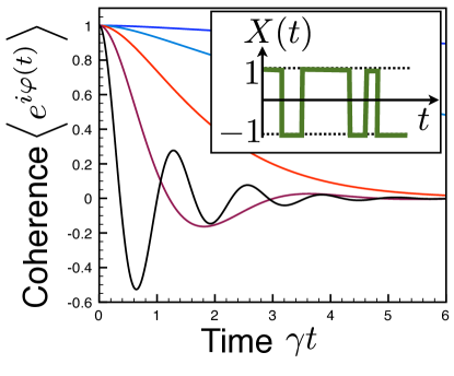
Figure 1: The coherence of a qubit subject to pure dephasing by classical telegraph noise (inset), for increasing coupling strength (top to bottom): $\alpha/\gamma=0.2,0.5,1,2.0,5.0$. Note the oscillations beyond the strong-coupling threshold $\alpha/\gamma=1$.

II.1 Classical telegraph noise as an example of non-Gaussian noise

Most discussions of dephasing are concerned with harmonic oscillator environments or their counterparts, Gaussian noise processes. Not only are these the simplest class of environments, but they also do describe many important physical examples. In addition, they often turn out to be good approximations even in cases where the microscopic Hamiltonian of the environment is not a sum of harmonic oscillators. In the case of noise processes, this can be understood essentially from the central limit theorem: If the process is a sum of many independent fluctuating contributions, then that sum will be Gaussian to a good approximation, even if the individual terms are not.

However, there are important exceptions, and a part of current research into quantum dissipative systems is directed towards such situations.

Here, we will illustrate the salient features by reviewing the simplest pedagogical example of a non-Gaussian noise process, namely telegraph noise. This is the name for a process $V(t)$ that can take only two values and randomly jumps between those values. Then, the distribution of possible values $V(t)$ at any given time $t$ is obviously not a Gaussian. The probability for these jumps to occur in a given time-interval is assumed to be independent of the previous history of the process, i.e. the process is of the “Markov” type.

There are many possible realizations for such a process, among them an electron tunneling incoherently between two different locations inside a crystal. Such an electron gives rise to an electric field that can shift the energy of another coherent quantum two-level system. The energy shift $V(t)$ of the two-level system will depend on the current position of the electron, and is thus of the random telegraph type. A qubit subject to these energy fluctuations will acquire a random phase, $\varphi(t)=-\hbar^{-1}\int_{0}^{t}V(t^{\prime})dt^{\prime}$, such that its coherence (the off-diagonal entry of the density matrix) is suppressed by the factor $\left\langle e^{i\varphi}\right\rangle$. It is our aim to describe the time-evolution of the qubit’s coherence.

Let us, for simplicity, assume that the jump rates between the two states are equal to $\gamma$, and the two possible values $V=\pm\hbar\alpha=\hbar\alpha X$ (with $X=\pm 1$) thus occur with equal probability. (It is easy to generalize the results below to the case of unequal rates). The correlation function for such a process is

$$\left\langle V(t)V(0)\right\rangle=\hbar^{2}\alpha^{2}e^{-2\gamma|t|}\,.$$ (1)

If $V(t)$ were a Gaussian process, this correlator alone would be sufficient to calculate the decay of the coherence. A Gaussian process with the correlator (1) is of the Ornstein-Uhlenbeck type. We would obtain:

$$\left\langle e^{i\varphi(t)}\right\rangle=\exp\left[-\frac{\alpha^{2}}{2\gamma}(t-\frac{1}{2\gamma}(1-e^{-2\gamma t}))\right]\,.$$ (2)

In that case, the decay of the coherence is monotonous in time. However, we will see that the true telegraph noise process induces a much more interesting behaviour. In the end, we will compare the coherences predicted by the two models.

In order to find the time-evolution of $\left\langle e^{i\varphi}\right\rangle$, we can express it through the time-evolution of the probability densities $p_{+}(\varphi,t)$ and $p_{-}(\varphi,t)$ that describe the probabilities of finding the telegraph process in state $+$ or $-$ and having, at the same time, a certain value $\varphi$ of the phase. The equations governing the time-evolution are of “Markov” type, i.e. they only depend on the current values of $p_{\pm}(\varphi,t)$:

$$\dot{p}_{\pm}(\varphi,t)=\pm\alpha\partial_{\varphi}p_{\pm}(\varphi,t)+\gamma(p_{\mp}(\varphi,t)-p_{\pm}(\varphi,t))$$

The phase evolves deterministically, $\dot{\varphi}=-\alpha X$, if the telegraph process is in the state $X=\pm 1$. As a consequence, the probability density is shifted to the left ($p_{+}$) or to the right ($p_{-}$), which is reflected by the drift term $\pm\alpha\partial_{\varphi}p_{\pm}$ on the rhs. The second part describes the possibility of jumping, with a rate $\gamma$, between those two states. Initially, both states $\pm$ have equal probability and the phase is zero: $p_{+}(\varphi,t=0)=p_{-}(\varphi,t=0)=\frac{1}{2}\delta(\varphi)$.

However, instead of solving these equations for the probability densities (which is easily done after Fourier transformation) we can take a short-cut. The trick is to write down equations of motion for $\left\langle e^{i\varphi}\right\rangle$ and $\left\langle Xe^{i\varphi}\right\rangle$, and to observe that these equations close. First, we find

$$\frac{d}{dt}\left\langle e^{i\varphi(t)}\right\rangle=i\left\langle\dot{\varphi}(t)e^{i\varphi(t)}\right\rangle=-i\alpha\left\langle X(t)e^{i\varphi(t)}\right\rangle\,.$$ (3)

In the next step, we have to take the time-derivative of $\left\langle Xe^{i\varphi}\right\rangle$. Here we can employ the fact that $X$ is a dichotomous process, i.e. $X^{2}\equiv 1$ is a constant. Therefore

$$\left\langle X\frac{d}{dt}e^{i\varphi}\right\rangle=-i\alpha\left\langle X^{2}e^{i\varphi}\right\rangle=-i\alpha\left\langle e^{i\varphi}\right\rangle\,.$$ (4)

We are still left, however, with the problem of evaluating $\left\langle e^{i\varphi}\frac{d}{dt}X\right\rangle$. We note first that the random process $dX/dt$ consists of a series of delta peaks, with prefactors $\pm 2$, corresponding to transitions from $X=-1$ to $X=+1$ and vice versa. We can express this by writing $dX/dt=-2XY$, where $Y$ is a Poisson process, consisting of uncorrelated delta peaks of weight $1$. The probability of observing a jump (i.e. one of these peaks) inside a time interval around $t$ is independent of the previous history $Y(t^{\prime})$ at times $t^{\prime}<t$, and thus also independent of $X$ and $\varphi$. Therefore

$$\left\langle e^{i\varphi}dX/dt\right\rangle=-2\left\langle e^{i\varphi}XY\right\rangle=$$

$$-2\left\langle e^{i\varphi}X\right\rangle\left\langle Y\right\rangle=-2\left\langle e^{i\varphi}X\right\rangle\gamma \,,$$ (5)

and we arrive at

$$\frac{d}{dt}\left\langle X(t)e^{i\varphi(t)}\right\rangle=-i\alpha\left\langle e^{i\varphi(t)}\right\rangle-2\gamma\left\langle X(t)e^{i\varphi(t)}\right\rangle\,.$$ (6)

Taking the derivative of Eq. (3), and inserting Eq. (6), we find that $\left\langle e^{i\varphi}\right\rangle$ obeys the equation of motion of a damped harmonic oscillator:

$$\frac{d^{2}}{dt^{2}}\left\langle e^{i\varphi}\right\rangle=-\alpha^{2}\left\langle e^{i\varphi}\right\rangle-2\gamma\frac{d}{dt}\left\langle e^{i\varphi}\right\rangle\,.$$ (7)

The solution of this equation (with the proper initial conditions $\left\langle e^{i\varphi}\right\rangle=1$ and $\left\langle Xe^{i\varphi}\right\rangle=0$) is:

$$\left\langle e^{i\varphi}\right\rangle=\frac{1}{2}e^{-\gamma t}\left\{\left[1+\frac{\gamma}{i\Omega}\right]e^{i\Omega t}+\left[1-\frac{\gamma}{i\Omega}\right]e^{-i\Omega t}\right\}\,,$$ (8)

with $\Omega\equiv\sqrt{\alpha^{2}-\gamma^{2}}$. This is the coherence of a two-level system subject to pure dephasing by random telegraph noise of strength $\alpha$ and switching rate $\gamma$ (see Fig. 1).

For strong damping (weak coupling), $\gamma>\alpha$, the fictitious harmonic oscillator is overdamped, $\Omega$ is imaginary, and the decay of $\left\langle e^{i\varphi}\right\rangle$ is monotonous, qualitatively similar to the expectation for dephasing by Gaussian noise. In contrast, for strong coupling, $\alpha>\gamma$, the coherence will display damped oscillations (i.e. it may become negative). This behaviour is qualitatively different from what would have been predicted in the case of a Gaussian random process (see Eq. (2) above). In fact, it cannot be mimicked by any Gaussian process, since there the coherence can never become negative! The frequency scale $\Omega$ of the oscillations becomes equal to the coupling strength $\alpha$ in the limit of a vanishing switching rate $\gamma\rightarrow 0$. This can be understood quite easily. In that limit, the positive and negative sign in $\varphi=\pm\alpha t$ each occurs with probability $1/2$, thus $\left\langle e^{i\varphi}\right\rangle=\frac{1}{2}[e^{i\alpha t}+e^{-i\alpha t}]=\cos(\alpha t)$.

In the particular limit of a very high switching rate, $\gamma/\alpha\rightarrow\infty$, we expect the Gaussian process to be a good approximation: In that limit, the phase is a sum over many small independent contributions (from small time-intervals of order $\gamma^{-1}$) and thus should become a Gaussian variable according to the central limit theorem, performing a close approximation to a random walk. Indeed, evaluating the exact result (8) for the coherence in the limit $\alpha/\gamma\rightarrow 0,\,\,\alpha^{2}t/\gamma={\rm const}$ (which implies $\gamma t\gg 1$), we find, to leading order in $\alpha/\gamma$:

$$\left\langle e^{i\varphi}\right\rangle\approx\left[1+\frac{\alpha^{2}}{4\gamma^{2}}\right]e^{-\frac{\alpha^{2}}{2\gamma}t}\,.$$ (9)

This coincides with the result for the corresponding Gaussian process, Eq. (2), evaluated in the same limit and to the same approximation.

In this example, we have thus found the coherence of a two-level system for a non-Gaussian process and learned that it can deviate qualitatively from that of a Gaussian process. Only in the limit of weak coupling, when the effect on the phase during one correlation time $1/\gamma$ of the fluctuations is very small, one can obtain the same results from a Gaussian process with the same correlator.

II.2 Quantum telegraph noise

We now want to ask about situations in which there is a quantum analogue of classical telegraph noise. This is in the spirit of the concept of ’Quantum Brownian motion’ 1983_CaldeiraLeggett_QuantumBrownianMotion , where one asks for a quantum model which will yield classical Brownian motion and velocity-proportional friction in the high temperature limit.

Possibly the simplest model is a single level onto which particles may hop. If we forbid multiple occupation, either by postulating interactions (hard), or by dealing with fermions and appealing to the Pauli principle (simple), then the occupation number of that level will fluctuate between $0$ and $1$. We have recently looked at the second case 2008_05_AbelMarquardt_QuantumTelegraphNoise , in a model where a single defect level is tunnel-coupled to an infinite reservoir of non-interacting fermions. The charge fluctuations of this level couple to the energy splitting of a qubit, thus giving rise to dephasing. This is a realistic model for describing the dephasing of charge qubits by two-level fluctuators, and various aspects and limiting cases of that model had been studied before 2002_06_PaladinoFazio_TelegraphNoisePRL ; 2005_08_Lerner_QuantumTelegraphNoiseLongTime ; 2006_03_GalperinAltshuler_NonGaussianQubitDecoherence ; 2006_01_SchrieflShnirman_DecoherenceTLS .

However, in 2008_05_AbelMarquardt_QuantumTelegraphNoise we provide an exact solution and evaluate it numerically to discuss the qubit dephasing at arbitrary times (not only in the long-time limit that had been tackled in 2005_08_Lerner_QuantumTelegraphNoiseLongTime ). The off-diagonal element of the density matrix of the qubit is suppressed by a factor $D(t)$ that may be written as a determinant in the single-particle Hilbert space of the fermionic bath (including the defect level):

$$D(t)=\det\left(1-\hat{n}+e^{i(\hat{H}_{B}-\frac{v}{2}\hat{Q})t}e^{-i(\hat{H}_{B}+\frac{v}{2}\hat{Q})t}\hat{n}\right).$$ (10)

Here $\hat{n}=f(\hat{H}_{B})$ is the single-particle density matrix (set by the Fermi distribution in the equilibrium case we are looking at). $\hat{Q}$ is the occupation operator of the single level, coupling to the qubit, and $\nu$ is the interaction strength. The results depend on the ratio $\nu/\gamma$, where $\gamma$ is the tunneling rate for an electron to escape from the defect level.

Figure 2: The coherence $D(t)$ for a qubit subject to quantum telegraph noise (see Eq. (10) and 2008_05_AbelMarquardt_QuantumTelegraphNoise ), for a low value of the temperature, $T/\gamma=0.2$, as a function of time (horizontal) and coupling strength $\nu/\gamma$ (vertical). $D(t)$ is displayed as a density plot, with the thick lines indicating $D(t)\equiv 0$. The fluctuator sits at $\epsilon=0$. (Note: $D(t)$ has been multiplied with a trivial phase factor to make it real-valued; see 2008_05_AbelMarquardt_QuantumTelegraphNoise for more details and related plots)

The classical result (8) is recovered in the high-temperature limit, justifying the name ’quantum telegraph noise’. Even at lower temperatures, there is always a threshold in $\nu/\gamma$ beyond which $D(t)$ displays the tell-tale oscillations that characterize dephasing by non-Gaussian noise in the strong-coupling regime. This is exemplified in Fig. 2, where we display $D(t)$ in the low-temperature limit. Thus, this model represents one of the rare cases in which the non-trivial features of dephasing by non-Gaussian fluctuations can be described exactly even deep in the quantum regime.

II.3 Decoherence by shot noise

When current runs through a quantum wire, the resulting current or charge fluctuations are due to discrete electrons and therefore non-Gaussian (and non-equilibrium) in nature. We can construct a simple model, relevant for charge-qubit readout, by postulating an interaction between a qubit and the charge fluctuations in some section of a nearby 1d ballistic quantum wire. Some current (driven by an applied voltage $V$) is injected into the wire through a beam splitter with transmission probability $\mathcal{T}$.

Our analysis of this model 2007_05_NederMarquardt_NJP_NonGaussian builds on the exact evaluation of a determinantal expression similar to Eq. (10). It reveals several interesting features: (i) In such a 1d system, the charge fluctuations in equilibrium (i.e. for zero voltage) are Gaussian, and only non-zero voltages will produce interesting deviations from Gaussian dephasing. (ii) The expression for the qubit’s coherence is closely related to full-counting statistics, and measuring its time-evolution may give access to that statistics at intermediate times, different from the usual long-time limit. (iii) For not too small interaction times, the results are essentially a function of $eVt$, where $V$ is the applied voltage. (iv) Again we find a certain ($V$-independent) threshold in the interaction strength, beyond which coherence oscillations set in.

A variant of this model has been realized recently in experiments: By coupling the quantum wire capacitively to one channel of an electron interferometer, it may be employed as a which-path detector. This concept has been implemented in the Heiblum group at the Weizmann Institute, making use of the electronic Mach-Zehnder interferometer (see below). The qubit’s coherence is then replaced by the interferometer’s interference contrast (visibility). Since the coupling between two adjacent edge channels in the Quantum Hall effect can become very large, that experiment has (apparently for the first time) entered a regime where the visibility oscillations associated to dephasing by non-Gaussian noise have been observed in an electronic interference experiment 2006_07_MZ_DephasingNonGaussianNoise_NederMarquardt .

III Dephasing in fermionic systems

III.1 The electronic Mach-Zehnder interferometer

Whereas the physics of decoherence has been studied in great detail for single particle systems, much remains to be learned in dealing with decoherence in many-particle systems. We refer the reader to 2006_04_DecoherenceReview for a brief review. In the past, we have studied several models to tackle the questions associated with this topic, including: A ballistic ring containing many electrons, coupled to a fluctuating quantum flux2002_Marquardt_AB_PRB , transport through a double dot interferometer subject to a noisy quantum bath 2003_Marquardt_DD_Interferometer , a many-fermion generalization of the Caldeira-Leggett model 2004_Marquardt_DFS_PRL ; 2004_Marquardt_DFS_LongVersion , decoherence by external quantum noise in an electronic Mach-Zehnder interferometer 2004_10_Marquardt_MZQB_PRL , and decoherence in weak localization 2005_10_WeaklocDecoherenceOne .

Of particular interest are electronic systems such as they occur in solid state transport interference experiments. Especially the first realization of the electronic Mach-Zehnder interferometer (MZI) (Fig.3) in the Heiblum group and subsequent experiments 2003_Heiblum_MachZehnder ; 2006_01_Neder_VisibilityOscillations ; 2008_02_Strunk_MZ_Coherence_FillingFactor ; 2008_03_Roche_CoherenceLengthMZ provide a particularly beautiful clean model system in which to study the effects of interactions and decoherence on the interference contrast in a many-fermion system .

Figure 3: (a) Scheme of the Mach-Zehnder interferometer. The two channels $1$ and $2$ of length $x_{L,R}$ and the corresponding chemical potentials $\mu_{L,R}$ are indicated. The electrons can tunnel at QPCs A and B, with tunnel amplitudes $t_{a}$ and $t_{b}$. By tuning the magnetic flux $\Phi$ through the interferometer, one observes an interference pattern $I(\phi)$. (b) The electron’s coherence, $G^{>}(\epsilon,x)/\nu(\epsilon)$, as a function of propagation distance, for various values of the energy $\epsilon$ (from top to bottom): $\epsilon/(q_{c}v_{F})=0,0.54,1.15,1.75,2.36,2.96$. The dashed, black line indicates the limit $\epsilon\rightarrow\infty$. Here, the interaction potential is $U_{q}=2\pi\alpha v_{F}\exp(-(q/q_{c})^{2})$, with $\alpha=3.0/2\pi$.

Experimentally, the MZI is realized by making use of integer quantum Hall edge channels, which are connected via quantum point contacts (QPCs), representing the beam splitters in the well known optical version of the interferometer. For our purposes, we will model this by assuming that there are two chiral electronic channels, being weakly tunnel-coupled to each other at two locations with tunneling amplitudes $t_{a}$ and $t_{b}$, respectively. Thus, we restrict our discussion to highly reflecting QPCs in order to employ perturbation theory (following 2006_09_Sukhorukov_MZ_CoupledEdges ; 2007_ChalkerGefen_MZ ). Applying a finite bias voltage $V$ between the channels leads to a current $I$ through the interferometer. There is an Aharonov-Bohm phase difference, such that $I(\Phi)$ becomes an oscillating function of the magnetic flux $\Phi$. Introducing the maximum and the minimum current with respect to $\Phi$, one may characterize the interference contrast via the so-called visibility $\mathcal{V}\equiv(I_{{\rm{\rm max}}}-I_{{\rm min}})/(I_{{\rm{\rm max}}}+I_{{\rm min}})$. The visibility can be used as a direct measure for the coherence of the system.

To take into account interactions in the chiral channels, one can employ the technique of bosonization. Then one only needs to obtain the electron Green’s function (GF) in channel $j\in(L,R)$, $G_{j}^{>}(x,t)\equiv-i\left\langle\hat{\Psi}(x,t)\hat{\Psi}^{\dagger}(0,0)\right\rangle$ and the corresponding hole GF $G^{<}(x,t)$. We can find 2008_06_Neuenhahn_UniversalDephasing_Short a rather intuitive expression for the visibility in terms of the GFs’ Fourier transform with respect to $t$ (here $T=0$):

$$\mathcal{V}=\frac{2|t_{a}t_{b}^{\ast}|}{|t_{a}|^{2}+|t_{b}|^{2}}\cdot\frac{\left|\int_{0}^{\delta\mu}d\epsilon\;G_{L}^{>}(x_{L},\epsilon)G_{R}^{<}(-x_{R},\epsilon-\delta\mu)\right|}{\int_{0}^{\delta\mu}d\epsilon\;\nu_{L}(\epsilon)\nu_{R}(\epsilon-\delta\mu)}\,,$$ (11)

where $G^{<}(x,\epsilon)=G^{>*}(x,-\epsilon)$ and
$\nu_{L,R}(\epsilon)=\left|G_{L,R}^{>(<)}(0,\epsilon)\right|$ for $\epsilon>0$ ($\epsilon<0$). There are contributions from all electrons inside the voltage interval, $\epsilon=0\ldots\delta\mu$, where $\delta\mu=q_{e}V>0$ is the bias between the left and the right arm of the interferometer. The propagation distance between the QPC’s in channel $j$ is denoted by $x_{j}$.

Obviously, the visibility only depends on a product of the electron- and the hole-GF. In order to understand the reason for this generic feature, one has to think about the nature of coherence in many body systems 2006_04_DecoherenceReview ; 2005_10_WeaklocDecoherenceOne . Let us think of an electron starting, for example in channel $R$ (Fig. 3). In the end we measure the current at the output port in channel $L$. When the electron arrives at QPC A it can be reflected, remaining in channel $R$, propagating there and finally tunneling into channel $L$, where it gets measured. In addition, the electron can immediatly tunnel at the first QPC, leaving a hole behind. After the propagation through channel $L$ the electron is counted at the output port. Loosely speaking, the action of QPC A turns the full electronic many-body state into a coherent superposition of many-body states, which are characterized by the status of all the electrons and holes in the system. Therefore scattering the hole destroys the coherent superposition just as well as scattering the electron itself.

Note that the coherence of the electron (hole) is completly encoded in the GF $G^{>(<)}(\epsilon,x)$. It yields the amplitude of an electron at energy $\epsilon$ propagating from $x=0$ to $x>0$.

III.2 Decoherence in chiral electron liquids

When applying the general discussion to a chiral 1d electron system, we first note that interactions lead to non-trivial effects only if one allows the interaction potential $U(x)$ to have some finite range, as emphasized in 2007_ChalkerGefen_MZ . Given the potential’s Fourier components, $U_{q}\equiv\int dx\,e^{-iqx}U(x)$, we introduce the dimensionless coupling strength $\alpha=\frac{U(q\rightarrow 0)}{2\pi v_{F}}$ (here $\hbar\equiv 1$). Besides that, we just assume the potential to fall off on a scale $q_{c}$ in momentum space.

In Fig. 3, we show an example of $G^{>}(\epsilon,x)$ as a function of $x$ for different energies $\epsilon$, obtained by numerically evaluating the exact bosonization solution. One can observe that it decays for increasing propagation distance $x$, reflecting the decoherence of the electron moving through the channel. Obviously the strength of the decoherence depends on the energy $\epsilon$. Two different energy regimes show up: For energies close to the Fermi edge, $\epsilon-\epsilon_{F}\ll q_{c}v_{F}$, the decoherence is suppressed, becoming stronger at larger energies. Thus the visibility $\mathcal{V}$ decays upon increasing the bias voltage $V$. In the limit of high energies, the coherence $\left|G^{>}(\epsilon,x)\right|$ becomes energy-independent.

In a recent work 2008_06_Neuenhahn_UniversalDephasing_Short , we have shown that one can apply a semiclassical approximation which gets exact in the limit of high-energy electrons and provides a very intuitive picture. The basic idea postulated in that work is a variant of the equation-of-motion approach to decoherence in fermionic systems 2004_10_Marquardt_MZQB_PRL ; 2006_04_MZQB_Long ; 2006_04_DecoherenceReview , and is related to functional bosonization: The propagating electron picks up a random phase originating from the potential fluctuations due to all the other electrons.

An unexpected nontrivial result of the analysis in 2008_06_Neuenhahn_UniversalDephasing_Short is that the high-energy electrons display a universal power-law decay of the coherence, i.e. $|G^{>}(\epsilon,x)|\propto 1/x$ for $x\rightarrow\infty$, with an exponent $1$ independent of interaction strength (at $T=0$). This can be connected to the universal low-frequency behaviour of the fluctuation spectrum that is observed in the electron’s moving frame of reference. (To avoid confusion, note that $|G^{>}(\epsilon,x)|\equiv 1$ in the absence of interactions!) Such a behaviour is in contrast to the low-energy (!) power-law decay of coherence of a non-chiral Luttinger liquid, where the exponent does depend on the interaction strength. Note that in the situation discussed here there is no decay at low energies, since we are dealing with a chiral Fermi liquid.

IV Conclusions

In this brief review, we have recounted some of our recent developments in the field of decoherence. Obviously, there are many problems that remain to be analyzed in the future. These include treating non-Gaussian noise in situations where only fully numerical methods may be applicable, and dealing with interacting electronic interferometers without assumptions like small tunnel coupling.

Acknowledgements. - We would like to acknowledge support through SFB/TR12, NIM, the Emmy-Noether program, and SFB 631.

References

- (1)
- (2) U. Weiss, Quantum Dissipative Systems (World Scientific, Singapore, 2000).
- (3) A. Stern, Y. Aharonov, and Y. Imry, Phys. Rev. A 41, 3436 (1990).
- (4) W. Zurek, Physics Today 44, 36 (1991).
- (5) H. P. Breuer and F. Petruccione, The Theory of Open Quantum Systems (Oxford University Press (Oxford), 2002).
- (6) A. O. Caldeira and A. J. Leggett, Physica 121A, 587 (1983).
- (7) B. Abel and F. Marquardt, arXiv:0805.0962 (2008).
- (8) E. Paladino, L. Faoro, G. Falci, and R. Fazio, Phys. Rev. Lett. 88, 228304 (2002).
- (9) A. Grishin, I. V. Yurkevich, and I. V. Lerner, Phys. Rev. B 72, 060509(R) (2005).
- (10) Y. M. Galperin, B. L. Altshuler, J. Bergli, and D. V. Shantsev, Phys. Rev. Lett. 96, 097009 (2006).
- (11) J. Schriefl, Y. Makhlin, A. Shnirman, and G. Schön, New Journal of Physics 8, 1 (2006).
- (12) I. Neder and F. Marquardt, New Journal of Physics 9, 112 (2007).
- (13) I. Neder, F. Marquardt, M. Heiblum, D. Mahalu, and V. Umansky, Nature Physics 3, 534 (2007).
- (14) F. Marquardt, in ”Advances in Solid State Physics” (Springer), Vol. 46, ed. R. Haug [cond-mat/0604626] (2007).
- (15) F. Marquardt and C. Bruder, Phys. Rev. B 65, 125315 (2002).
- (16) F. Marquardt and C. Bruder, Phys. Rev. B 68, 195305 (2003).
- (17) F. Marquardt and D. S. Golubev, Phys. Rev. Lett. 93, 130404 (2004).
- (18) F. Marquardt and D. S. Golubev, Phys. Rev. A 70, 053609 (2005).
- (19) F. Marquardt, Europhysics Letters 72, 788 (2005).
- (20) F. Marquardt, J. v. Delft, R. Smith, and V. Ambegaokar, Phys. Rev. B 76, 195331 (2007).
- (21) Y. Ji, Y. Chung, D. Sprinzak, M. Heiblum, D. Mahalu, and H. Shtrikman, Nature 422, 415 (2003).
- (22) I. Neder, M. Heiblum, Y. Levinson, D. Mahalu, and V. Umansky, Phys. Rev. Lett. 96, 016804 (2006).
- (23) L. Litvin, A. Helzel, H. Tranitz, W. Wegscheider, and C. Strunk, Phys. Rev. B 78, 075303 (2008).
- (24) P. Roulleau, F. Portier, P. Roche, A. Cavanna, G. Faini, U. Gennser, and D. Mailly, Physical Review Letters 100, 126802 (2008).
- (25) E. V. Sukhorukov and V. V. Cheianov, Phys. Rev. Lett. 99, 156801 (2007).
- (26) J. T. Chalker, Y. Gefen, and M. Y. Veillette, Physical Review B 76(8), 085320 (2007).
- (27) C. Neuenhahn and F. Marquardt, arXiv:0806.121 (2008).
- (28) F. Marquardt, Phys. Rev. B 74, 125319 (2006).