PHotometry Assisted Spectral Extraction (PHASE) and identification of SNLS supernovae

Abstract

Aims. We present new extraction and identification techniques for supernova (SN) spectra developed within the Supernova Legacy Survey (SNLS) collaboration.

Methods. The new spectral extraction method takes full advantage of photometric information from the Canada-France-Hawaï telescope (CFHT) discovery and reference images by tracing the exact position of the supernova and the host signals on the spectrogram. When present, the host spatial profile is measured on deep multi-band reference images and is used to model the host contribution to the full (supernova + host) signal. The supernova is modelled as a Gaussian function of width equal to the seeing. A $\chi^{2}$ minimisation provides the flux of each component in each pixel of the 2D spectrogram. For a host-supernova separation greater than $\stackrel{{\scriptstyle>}}{{{}_{\sim}}}$ 1 pixel, the two components are recovered separately and we do not use a spectral template in contrast to more standard analyses. This new procedure permits a clean extraction of the supernova separately from the host in about 70% of the 3rd year ESO/VLT spectra of the SNLS. A new supernova identification method is also proposed. It uses the SALT2 spectrophotometric template to combine the photometric and spectral data. A galaxy template is allowed for spectra for which a separate extraction of the supernova and the host was not possible.

Results. These new techniques have been tested against more standard extraction and identification procedures. They permit a secure type and redshift determination in about 80% of cases. The present paper illustrates their performances on a few sample spectra.

1 Introduction

Observing Type Ia supernovae (SNe Ia) for the purpose of constraining cosmological parameters is now a mature activity. Large-scale projects of detection and spectrophotometric follow up of hundreds of SNe Ia from ground-based telescopes reach completion today (Astier et al., 2006; Wood-Vasey et al., 2007), and future SNe Ia surveys will bring this number up to several thousand. These current and future surveys yield and will yield new samples of SNe Ia observations of unprecedented number and quality. Extracting the most possible out of these exceptional sets of SNe Ia data is a challenge for the teams involved in these projects.

At redshifts greater than $z\stackrel{{\scriptstyle>}}{{{}_{\sim}}}0.2$, the problem of spectroscopically identifying supernovae is more challenging than it is at low redshift. At low redshift, galaxies have a larger angular size, so at the position of the supernova (SN) the spectrograph slit usually contains little contaminating host galaxy light. As redshift increases, apparent galaxy sizes decrease and the galaxy light can be comparable to, or dominate, the supernova light at a given position. For observations of high-redshift supernovae, new techniques are therefore required to efficiently recover the supernova signal (see e.g., Blondin at al. 2005).

Currently, the SNe Ia spectroscopic sample of the Supernova Legacy Survey (SNLS) represents more than 500 spectra taken from 8-10m diameter telescopes, both in the Southern and Northern hemispheres (VLT, Gemini N and S, Keck-I and -II) during large observing programmes of hundreds of hours run from 2003 up to the present day. The spectra obtained with such programmes sample a large fraction of the wavelength space (depending on the instrument used) in the visible. They have restframe phases comprised between -15 and +30 days and sufficient signal-to-noise ratios (S/N) for an unambiguous identification in $\sim 80$% of cases.

Besides their use for cosmological purposes – that is identification of the supernova type and determination of their redshift for their inclusion in a Hubble diagram, these spectra contain valuable information to understand the nature and the diversity of SNe Ia and test the adequacy of using them as “standardisable”, if not standard, candles. As an example, Guy et al. (2007) have implemented a number of SNLS spectra in the training set of the spectrophotometric template SALT2, one of the fitters used to fit the light curves of SNe Ia in the 3rd year SNLS Hubble diagram. Moreover, comparison of the spectral properties of these high-redshift ($<z>\sim 0.5-0.6$) supernovae with their low-$z$ counterparts (from, e.g., the spectral time series currently collected by the SN Factory experiment, see Aldering et al. 2002 and Matheson et al. 2008) should help in understanding possible evolutionary effects in SNe Ia populations (Bronder et al., 2008; Balland et al., 2006, 2007; Blondin et al., 2006; Garavini et al., 2007; Foley et al., 2008). Another interesting particularity of the SNLS spectral sample is that, due to the high average redshift of the SNLS SNe Ia, the ultraviolet (UV) part of the supernovae spectra down to $\approx 3200$ $\AA$ is accessible for a large number of supernovae at various phases (see, e.g., Ellis et al. 2008 for a study of the UV features of 36 SNLS-Keck spectra). This is of particular interest as it has been suggested that possible evolution with redshift, due to different progenitor metallicities at low and high redshift, might be imprinted in the spectral features of this region of the spectrum (Hoeflich et al., 1998; Lentz et al., 2000). Optimal extraction of SNLS spectra and their identification are thus not only a crucial step in building the Hubble diagram but are also crucial for their subsequent use in studies of the physics of SNe Ia.

Standard analyses of spectra are often based on the Horne’s extraction method (Horne, 1986) that uses the spatial profile of the source light to perform an optimal (minimum-variance unbiased) spectral extraction. A drawback of this approach is that only mild geometrical distortions due, for example, to flexure of the instrument are corrected for (however, see Marsh (1989) for an extension of Horne’s method suited for highly distorted spectra). Another major problem of this approach is that it does not permit the separate extraction of the supernova from the host signal, except if the two components (SN and host galaxy) are well separated on the spectrogram (and in this case, correlations between the host and the SN spectra are usually unavoidable, even if the extraction window is adjusted to maximise the supernova signal and minimise the host contamination). In most cases, the SN/host separation is performed a posteriori by fitting a two-component model (built from a supernova and a galaxy template), the contribution of each component to the total model being evaluated by a $\chi^{2}$ minimisation (Howell & Wang, 2002; Howell et al., 2005; Balland et al., 2006, 2007). As the model is built from a (limited) set of templates, the SN and host spectra obtained by this procedure are strongly model-dependent and provide at best a hint of the host contribution to the full spectral model. Ellis et al. (2008) have developed an improved separation technique based on fitting synthetic galaxy spectra to the host photometry measured on reference images. By doing so, they still rely on a spectral model to estimate the host contribution to the full signal. Blondin et al. (2005) use a convolution technique to simultaneously recover a host-free PSF-like SN component and its background galaxy spectrum. This method does not use any spectral template for the host modeling and thus improves over more classical extraction techniques. However, this technique is sensitive to the width of the spatial resolution Gaussian kernel used to recover the background (host) component. The width has to be tuned by the user and highly depends on the spatial extension of the host galaxy. Moreover, the method does not use photometric information that potentially goes along with the spectrum.

To circumvent these drawbacks and improve over standard extraction methods, we have developed a dedicated reduction and extraction pipeline, called PHASE (PHotometry Assisted Spectral Extraction). This new technique uses photometric priors from Canada-France-Hawaï Telescope (CFHT) detection images obtained with megacam (Boulade et al., 2003) to derive the exact trace of the supernova on the spectrogram. This trace is then used as a guide for extraction. Here, ”true” photometric information of the host contribution in each pixel, obtained from CFHT Legacy Survey (CFHTLS) deep reference images in various photometric bands, is used, when possible, at the stage of the extraction. In the favourable cases of large enough host/SN separation, we do not use a spectral template to model the host galaxy contribution. The spatial profile of the host, measured on the reference image along columns parallel to the slit, is used instead.

Technical choices sometimes different from the standard ones have been investigated to select the most efficient and robust ones necessary for a clean and final extraction. We have automated the reduction pipeline as much as possible to reduce the operator work load as well as unavoidable human errors. Besides the technical aspects of this new approach, in all the reduction and extraction processing, one of our main concerns is to control and propagate the noise level estimation from raw data up to the final reduced spectrum in the cleanest way possible. In particular, re-sampling of data that introduce correlations among pixels is kept to a minimum and is done as late as possible in order to preserve as long as possible the independence of pixels. This allows us to extract a clean, optimal signal-to noise spectrum, and in about 70% of the currently treated spectra (3rd year VLT spectra of the SNLS, see Balland et al. 2008), this is a host-free supernova spectrum. We discuss in this paper the improvement in terms of S/N over more standard extractions.

Identification of the supernova type is then performed by combining spectral and light curve informations using the spectrophotometric template SALT2 developed by Guy et al. (2007). In this approach, all available information on a given supernova (both photometric and spectral) is used to ease the identification. This contrasts with the more straightforward method of a two component spectral model. As underlined in, e.g., Hook et al. (2005); Lidman et al. (2005); Balland et al. (2006, 2007), a difficulty of this approach is the possible confusion of SNe Ia spectra past maximum with Type Ic supernovae (SNe Ic) at an earlier phase. Using the photometric phase as a constraint is crucial to alleviate this degeneracy.

In this paper, we present the techniques developed for the spectral extraction and the identification of our spectra. We illustrate our results with a few sample spectra obtained at VLT, as part of two large spectroscopic programmes running from June 2003 to September 2007, that are being processed using this technique (Balland et al., 2008). In Sections 2, 3 and 4, we describe the PHASE technique and test it on simulated data. In Section 5, we illustrate PHASE results and discuss the improvements over standard extractions. In Section 6, the identification method of SNLS spectra using the SALT2 spectral template is described and results are discussed on a few examples. Discussion and conclusion are in Section 7 and Section 8, respectively.

2 2D spectrum calibration using PHASE

Spectral extraction usually requires human interaction to define the locus on the frame of the object to be extracted/measured. Spectra are often distorted along the dispersion axis, and the extraction algorithm must be sophisticated enough to find and follow the source trace along this axis. Technically, one first specifies the source location as a set of pixel coordinates that is subsequently corrected during the extraction process.

Such a procedure, if relevant in the case of resolved sources, is not wanted for overlapping sources such as a point-like supernova on its extended host galaxy. Beside the fact that both the supernova and its underlying host light are extracted together , the position and slope of the supernova trace itself can not be easily retrieved. Indeed, usual algorithms such as Horne (1986) seek the flux centroid, and might end up pushing the position of the supernova towards the galaxy brighter core.

In order to avoid these pitfalls, we use the fact that SNLS produces deep images of the regions in which supernovae explode. The supernova location and magnitudes in four photometric bands ($g_{M},r_{M},i_{M},z_{M}$) are known. Consequently, given this photometric information, it is possible to locate the supernova on the spectrogram at sub-pixel accuracy, to trace its spectrum, and to perform an optimised extraction able to separately measure the supernova and host galaxy fluxes along the CCD frame.

2.1 FORS1 long slit spectra calibration

During the first VLT large programme (2003-2005), SNLS spectra have been acquired in long slit mode (LSS) with the FORS1 instrument in service mode. A preliminary assessment of the spectroscopic data was performed within a few days in order to confirm the validity of the candidate. For this “real-time” analysis of the spectra (Basa et al., 2008), the SNLS team used a combination of a dedicated reduction pipeline based on the ESO-MIDAS software, a proper Horne (1986) extraction package and a template supernova and galaxy fitting software (${\cal SN}$-fit, Sainton 2004; Balland et al. 2006) to perform an on-line identification and redshift measurement.

The FORS1 detector is a 2k$\times$2k CCD. To acquire supernova spectra, we used it with the standard collimator and mainly with the 300V grism, along with the GG435 order-sorting filter. The pixel scale is $0.2^{\prime\prime}$ along the spatial axis ($Y$), and $2.65\,\AA$ along the dispersion axis ($X$). PHASE has initially been implemented to treat the long slit spectra taken on FORS1. The multi-object (MOS) mode is currently marginally supported (the majority of standard stars were observed in MOS mode) but its full support is in progress and will be used to extract the MOS spectra, mostly obtained during the second SNLS-VLT large programme (2005-2007).

In the following, we focus on the main features of the data processing. Technical details can be found in Baumont (2007).

For calibration purposes, we built bias master frames as median of bias frames grouped per trimester ($\sim 50$ frames). The scan subtracted r.m.s. of each pixel value was clipped from $8\sigma$ deviant events, where $\sigma$ is the read-out-noise (RON) level taken from the raw frame header. With this threshold, most cosmic rays were efficiently removed.

Normalised flat-fields were produced by grouping frames per run (per lunation). After an iterative median with a $5\sigma$ clipping suitable for removing most of bad pixels, the internal lamp spectrum was estimated in 16 spatial bands along the $Y$ axis and used to produce normalised flat-fields that reflect sensitivity fluctuation patterns in those regions.

The dispersion function for science calibration was computed using a least square technique. The pixel position $X_{i,j}$ of 14 isolated emission lines of Hg, He and Ar was measured in 16 regions and averaged along the Y axis. Those lines were selected as the brightest and least blended ones. A set of nine dispersion coefficients (4th order in $X^{i}$, 2nd order in $Y^{i}$ and in $XY^{i}$) were adjusted to the $X_{i,j}$ values. This set turned out to be adequate for reproducing the dispersion solution. The 4th order coefficient $C_{x^{4}}$ along X has been added (it is not used by the Real-Time ESO pipeline) to further reduce the residuals. The residual r.m.s. is typically $0.2\,\AA$ and reaches $0.8\,\AA$ at the borders of the frame.

We chose to use a single response function per UT (FORS1 moved from UT1 to UT2 on June 2005) by combining all individual response functions derived for every standard star observation. With this procedure, the night to night sky transparency variation is not corrected for. We prefer to use a uniform, easy to control, average calibration for the full set, rather than calibrate an observation using the response function of a different night (ESO does not perform standard star observations for every night). As SNLS spectra are primarily used for the purpose of identification, we do not need absolute spectrophotometric calibration. Second order residual flux was sometimes found for the bluest standard star spectra. In this case, we estimated it and accordingly corrected the response function. The average $H_{2}0$ and $O_{2}$ atmospheric absorption spectra were computed in appropriate bands ([5800:6000], [7100:7350], [8100:8400], [8900:9850] $\AA$ for $H_{2}O$, and [6250:6350], [6800:7000], [7550:7750] $\AA$ for $O_{2}$) and used for further correction (see Section 5.1). As for the instrumental response, we used an average spectrum of the absorption, computed as the average ratio of the observed spectrum to the reference spectrum of the standard star, multiplied by the instrumental response interpolated in a given absorption band.

2.2 Combined 2D spectrogram

In general, we took $N_{img}$=2 to 5 exposures of 900s of our targets, with small offsets along the slit. We combined these $N_{img}$ frames of a given target to produce a clean, cosmic free sky subtracted 2D spectrogram to be used for extraction.

For cosmic ray removal prior to extraction, we used a temporal median filtering. The sky spectrum was obtained in 16 spatial regions by an iterative median projection along the $Y$ axis. These regions are of equal width and cover the full extension of the CCD along the $Y$ axis. Bright sources were detected as rows containing more than 5% of 5$\sigma$ deviant pixels and were avoided. The $16$ sky spectra were then averaged in wavelength space to yield the sky spectrum model for sky subtraction. Note that bias subtraction and flat-fielding were applied simultaneously during the first projection along $Y$ in the iterative process.

For a given SN candidate, bias subtraction, flat fielding and sky subtraction was then performed on each set of $N_{img}$ pixel values. Then a robust, seeing-weighted average of each calibrated set of pixels was applied to obtain one single output pixel value. The seeing was computed from the active optic wavefront sensor system on the guiding star, recorded in the ESO logs of observation. In rare cases (for a few standard star observations), those guiding star logs are lacking and the Differential IMage Monitor (DIMM) value was used instead. This latter value is accurate within 20%.

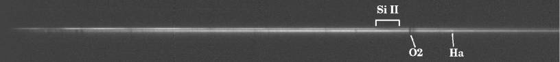
Figure 1: PHASE 2D combined spectrograms for SN 04D1dc. Top: the SN (top) and host (bottom) spectra after reduction. The main noticeable features in the SN and host spectra are indicated. Bottom: the corresponding 2D noise map, including the sky model. Spectra range from 4200 $\AA$ (left) to 9000 $\AA$ (right). Note the atmospheric absorption features affecting both the SN and host spectra.

Figure 1 shows the PHASE output 2D frames for SN 04D1dc taken as an illustration of the results produced by the reduction technique presented above. SN 04D1dc is a Type Ia supernova (SN Ia) at maximum light at $z=0.211$ well separated from its host core ($d_{SN-host\ centre}=1.18^{\prime\prime}$). The top panel shows the well separated SN (top) and host (bottom) spectra. Sky subtraction residuals appear as vertical narrow bands slightly visible at the locus of the most luminous sky emission. Atmospheric absorption features affecting both spectra are clearly seen at several places, such as the strong $O_{2}$ absorption at 7600 $\AA$. The emission and absorption features of the SN spectrum are seen as a modulation in the intensity of the top spectrum. The deep Si ii absorption at $\sim 6150$ Å  is visible to the blue part of the $O_{2}$ absorption (see labels in top panel of Fig. 1). In the host spectrum, H $\alpha$ emission is seen as a bright spot longward of $O_{2}$. Confusion of an emission line with a cosmic is very unlikely (a cosmic hit could mimic an emission line and extend spatially but it should be faint enough for it not to have been rejected, i.e. $<5\sigma$ of the average sky background). However, at high redshift ($z\geq 0.8$), the host flux is weak and it is more difficult to tell from the sole 2D spectrum whether a given spot is an emission line, a statistical fluctuation, or a cosmic residual. In the present case, we can check in the 2D noise map shown in the lower panel of Fig. 1 that the observed bright spot in the spectrum is not a cosmic subtraction residual. Indeed, if a cosmic hit the CCD at this location, it would be present in this 2D noise map, which is not the case. This illustrates how inspection of the 2D noise map helps at discriminating true host lines from cosmic hits.

3 A model for PHASE extraction

The basic idea for the extraction from the clean 2D spectrogram is to define beforehand the distribution of the sources that we expect to find in the frame and to recover their exact position (or trace) on the spectrogram. To achieve this, we rely on the comparison between the source spatial profiles obtained from deep CFHTLS reference images in three megacam photometric bands ($g_{M}$, $r_{M}$ and $i_{M}$ with Grism 300V) along the slit direction (the photometric profiles), with the corresponding profiles obtained from the VLT Long Slit spectrograms (the spectroscopic profiles). Then, given the expected spatial profile of the sources, a least square linear inversion of the pixel counts on each column, corresponding to a given $\lambda$, gives the flux of every component at this wavelength. In the following, we describe how we implement this procedure in PHASE.

3.1 Photometric priors

To built the photometric profiles, we project the region of the sky covered by the slit at its position angle from the deep reference images in all of the megacam photometric filters covered by the FORS1 order-sorting filter used (i.e, g_M, r_M and i_M for GG435 used with the 300V grism). This is done using SWarp (Bertin & Tissier, 2007). This yields three 1D spatial profiles that correspond to the expected galactic profiles in each filter.

The supernova coordinates, accurately measured when building its light curves, are used to place the supernova component on these profiles. Given that supernovae are point-like sources, the supernova component is modelled as a Gaussian profile whose width is the average seeing of the spectroscopic observation. As the supernova flux is not accounted for in the CFHTLS deep reference images, we add it “by hand” to the photometric profiles. To do this, the flux in each band is interpolated from the supernova light curves at the time of spectroscopy.

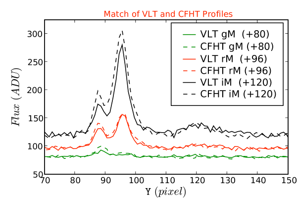
Figure 2: Match of the VLT (solid lines) and the CFHT (dashed lines) spatial profiles of SN 04D4it in three photometric bands (from bottom to top: $g_{M}$, $r_{M}$, $i_{M}$) arbitrarily shifted with respect to zero flux for the sake of clarity. The VLT profiles are obtained by averaging the spectrum in each photometric band. The CFHT profiles are measured on deep reference images. The correlation function of the two profiles is computed for each band and the spatial shifts are derived at the maximum of the correlation functions.

The photometric profiles are then compared to the spatial profiles averaged on the 2D VLT spectrogram in wavelength ranges corresponding to the photometric bands. For each band, the spatial shift between the two derived profiles (photometric and spectroscopic) is then computed at the maximum of their correlation function. Figure 2 illustrates the result of matching the VLT (solid lines) and the CFHT (dashed lines) profiles in $g_{M}$, $r_{M}$ and $i_{M}$ (from bottom to top) for SN 04D4it, chosen as a test case. Correlating the two profiles yields one shift for each photometric band whose mean $\lambda$ corresponds to a given column $X_{Band}$ of the spectrogram. Performing a linear fit of these shifts as a function of $X$ yields two parameters:

• 1) the spatial shift between the supernova location and the central row of the spectrogram, at the central column, and

• 2) the slope of the supernova location along the dispersion axis $X$.

The maximum tolerated spatial shift is 20 pixels. In average, the slope is of $10^{-3}$ pixel/pixel, corresponding to a 2 pixel drift from border to border of the frame.

This procedure hence allows us to measure precisely (at sub-pixel accuracy) the position and slope of the sources spectral trace on the 2D spectrogram. We now use this information to perform the extraction.

3.2 Building a multi-component model

For each column flux $F_{i}({\tt Y})=F({\tt X}_{i},{\tt Y})$ of the 2D spectrogram, we build a $N$-component spatial model as the sum of the profiles $\mathcal{C}_{k}({\tt Y})$ of individual objects in the slit, shifted by a quantity $\delta{\tt Y}_{i}$ according to the previously derived trace equation. Their total flux is normalised to unity. A flux $f_{k}$ is assigned to the $k^{th}$ component of the model and a uniform “background” component is added to account for possible sky subtraction residuals. The model for each column $i$ reads:

$${\mathcal{M}}_{i}({\tt Y})=\sum_{k}f_{k}{\mathcal{C}}_{k}({\tt Y}-\delta{\tt Y}_{i}).$$ (1)

The flux $f_{k}$ of each component is estimated by a $\chi^{2}$ minimisation where:

$$\chi^{2}=\sum_{j}\Big{(}\frac{F_{i}({\tt Y}_{j})-{\mathcal{M}}_{i}({\tt Y}_{j})}{\sigma_{j}}\Big{)}^{2}.$$ (2)

Here, $\sigma_{j}$ is the error associated with the column pixel data. The minimisation condition is equivalent to solving the following equation for each column:

$$\left[\begin{array}[]{ccc}\sum_{j}\frac{\mathcal{C}_{0}({\tt Y}_{j}^{\prime})^{2}}{\sigma_{j}^{2}}&\cdots&\sum_{j}\frac{\mathcal{C}_{0}({\tt Y}_{j}^{\prime})\mathcal{C}_{N}({\tt Y}_{j}^{\prime})}{\sigma_{j}^{2}}\\ \vdots&\ddots&\vdots\\ \sum_{j}\frac{\mathcal{C}_{N}({\tt Y}_{j}^{\prime})\mathcal{C}_{0}({\tt Y}_{j}^{\prime})}{\sigma_{j}^{2}}&\cdots&\sum_{j}\frac{\mathcal{C}_{N}({\tt Y}_{j}^{\prime})^{2}}{\sigma_{j}^{2}}\end{array}\right]\left[\begin{array}[]{c}f_{0}\\ \vdots\\ f_{N}\end{array}\right]=$$

$$\hskip 142.26378pt\left[\begin{array}[]{c}\sum_{j}\frac{\mathcal{C}_{0}({\tt Y}_{j}^{\prime})F_{i}({\tt Y}_{j})}{\sigma_{j}^{2}}\\ \vdots\\ \sum_{j}\frac{\mathcal{C}_{N}({\tt Y}_{j}^{\prime})F_{i}({\tt Y}_{j})}{\sigma_{j}^{2}}\end{array}\right],$$

where ${\tt Y}_{j}^{\prime}={\tt Y}_{j}-\delta{\tt Y}_{i}$ corresponds to the profiles shifted according to the trace inclination.

Much care must be taken to model the source profiles, since their accuracy will determine the quality of the extracted spectra. In particular, overlapping sources is a source of anti-correlated noise among components.

3.2.1 Setting the galaxy profiles

If the extraction window is narrow enough to ensure that no field galaxy other than the host is present, the galaxy profile and the supernova Gaussian can be used to perform an extraction with only two components (plus a uniform background component).

However, using a wide extraction window is preferable for a better sky residual estimation. This often implies that other object spectra are present in the window. Even in the case of a narrow extraction window, close galaxy pairs are sometimes present. In all these cases, we need to define a multi (greater than 2) component model. Moreover, for resolved spiral galaxies, the spiral arm spectrum is not the same as the core spectrum. In particular, nebular emission lines are much stronger in the arms due to the enhanced star burst activity. The H ii regions, ionised by the strong UV radiation from young and massive stars, produce these nebular emission lines (Osterbrock, 1989). Improper modeling of the arm and core structure as a single component leads PHASE to fail to assign the correct flux to the SN and to the galaxy. At the wavelengths of these nebular emissions, the host spatial profile does not correspond to the host profile averaged over the whole spectral range. In the case of an SN located in one arm, using the average profile to model the host would lead to underestimate the host flux at these wavelengths, and consequently, to overestimate the supernova flux. In such cases, it is necessary to model the arms and the core as two different components. Considering that high-redshift host galaxies are usually unresolved above a redshift of 0.7, we distinguish 3 types of galaxy profiles:

• $PSF$ : unresolved, point-like galaxies.

• $EXT$ : extended, regularly shaped profiles, e.g. ellipticals.

• $Mix$ : irregularly shaped profiles, e.g. galaxies with spiral arms. In practise, this profile is modelled as a PSF plus an EXT profiles.

In PHASE, cuts on flux, galactic compactness, extension minimum level and colour variation between the central Gaussian core (at seeing width) and the possible extension (e.g., arms) can be adjusted to favour one type over the others and thus adapt to the specific extraction case encountered. Nevertheless, default cuts are set to permit an automatic treatment of most spectra. Their values are chosen to yield the host type model (Mix, EXT or PSF) giving the best extraction (avoiding host contamination and degeneracy between the SN and host components) in most cases. For extended sources, we use the “bolometric” profile (that is the sum of the galactic profiles in all covered filters) as a model. In order to use a noiseless extraction profile, it is filtered with a Gaussian of width half the seeing, oversampled at a tenth of a pixel to ease the subsequent shifting of the profile to follow the trace slope. Note that using the projected 1D profile is a source of confusion when close pairs of galaxies happen to connect once projected along the given polar angle. However, sources are well defined for the subsequent extraction in $\sim$95% of the cases, and this is not a major concern.

3.2.2 Modelling the SN component

As mentioned in Section 3.1, the candidate supernova is an additional point-like source at the estimated position and of width equal to the seeing. The seeing variation with wavelength was estimated from standard star observations, as a power law of index $-0.3$. This corresponds to a $\sim 20$ % variation of the Full Width at Half Maximum (FWHM) from 4000 Å  to 9200 Å. Note that our power law value differs from $-0.2$, the value expected when assuming Kolmogorov turbulence (Schroeder, 1987) but is in agreement with the value found by Blondin et al. (2005) on FORS1 spectra. Note that we use this law for a distant PSF host as well. However, applying the same correction to extended sources would require a reference image of better seeing, and would only have a minor effect on the profile, so we do not perform it.

To avoid degeneracy between two overlapping point-like sources (e.g., the supernova and an unresolved host galaxy), a cut of a fifth of the seeing is imposed on the separation of the two point-like sources. For separation values lower than this cut, the SN component is merged to the unresolved galaxy and no separate extraction is possible. As expected, this situation occurs with increasing frequency at higher redshifts and only the sum of the supernova and of the host spectra can then be obtained. This situation occurs in about 30% of cases (see Balland et al. 2008) and is further referred to as the “SNGAL” case. However, the faintest hosts are not identified as sources since their level does not reach the detection threshold fixed in PHASE, and their spectra will only slightly contaminate the SN signal. When such a case occurs (or when a clear separation between the SN and the galaxy exists), we refer to it as a “SN” case.

4 Testing the validity of PHASE extractions

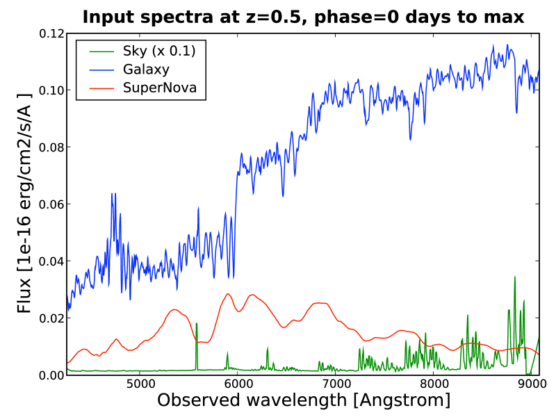
Figure 3: The host (blue) and sky (green) spectra used in the simulations testing the validity of PHASE extractions. The host is a Sb type from Kinney et al. (1996) and the sky background is taken from a real FORS1 exposure and is used to model the noise of the 2D input spectra. The flux of the Sb template is scaled to the one of NGC 6181 (Kennicutt 1992) at a distance of 34 Mpcs and its spatial profile on the synthetic 2D spectrogram is fixed from the angular size of NGC 6181 using the surface brightness profile of Ratnatunga et al. (1999). The supernova spectrum is modelled from the templates of Nobili et al. (2003), with phases ranging from -10 to 10 days. Here, the supernova template at maximum light is shown (red line) as an example.

In order to assess the validity of PHASE extractions, we have performed a series of simulations to test the impact of various parameters (supernova/host separation, phase and redshift of the supernova, seeing) on the recovered flux for each component. We start from Nobili et al. (2003) SNe Ia template spectra with phases ranging from -10 to +10 days relative to maximum light. We assume that the supernova host is resolved and use the Kinney et al. (1996) Sb template to model its spectral energy distribution. We follow Blondin et al. (2005) and generate the input synthetic 2D spectra (combined and sky background subtracted, for 3 exposures of 750 seconds) within the FORS1 instrumental environment. The profile of the host galaxy on the 2D synthetic spectrogram is fixed from the angular size of NGC 6181 (Kennicutt, 1992) and using, as in Blondin et al. (2005), the Ratnatunga et al. (1999) surface brightness profile. The flux of the host template is scaled to the one of NGC 6181 at a distance of 34 Mpcs. A model for the sky background (taken from a real FORS1 exposure) is used to model the noise of the input 2D spectra (in addition to the RON and to the shot noise of the sources). A curvature of the spectral trace (not accounted for during PHASE extraction) is modelled, introducing a 0.1 pixel offset from centre to border of the dispersion axis, consistent with the FORS1 curvature measured on standard star exposures. Figure 3 shows the input host and sky spectra, as well as the supernova spectrum at maximum light, for $z=0.5$.

We extract the signal with PHASE, imposing the photometric model. We perform 3 sets of simulations varying either the redshift ($0.2<z<1$), the SN phase ($-10<\phi<+10$ days) or the seeing ($0.4^{\prime\prime}<FWHM<1.4^{\prime\prime}$). In each case, the host/SN separation $d_{SN/Host\ centre}$ varies between 0 and 2^′′. The non-varying parameters are set to the default values $z^{0}=0.5$, $d_{SN/Host\ centre}^{0}=1^{\prime\prime}$ and $FWHM^{0}=0.75^{\prime\prime}$.

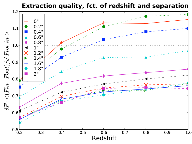
Figure 4: Residual $\delta F$ of a PHASE extraction performed on simulated data as a function of redshift. Values of $\delta F$ lower than 1 indicate that the flux has been recovered to the statistical noise limit. Symbols show $\delta F$ values for SN/host separations ranging from 0 to 2^′′. For $z>0.5$ and $d_{SN/Host\ centre}<0.4^{\prime\prime}$, $\delta F$ is greater than 1 as the galaxy becomes unresolved so that, for low separation, the degeneracy between the two component profiles is high. In practise, in such cases, PHASE would extract the two components together and not separately.

To evaluate the quality of the flux recovery, we adopt the criterion of Blondin et al. (2005) based on the residual $\delta F=|F_{out}-F_{in}|/\sqrt{(}F_{tot,in})$, where $F_{out}$ is the recovered supernova flux, $F_{in}$ the input supernova flux, and $F_{tot,in}$ takes into account the supernova+underlying host+sky background. If $\delta F<1$, the input signal has been restored to the statistical noise limit. Figures 4 to 6 present $\delta F$ as a function of redshift, phase and seeing. We see in Fig. 4 and 5 that PHASE recovers the correct flux ($\delta F<1$) for supernova-host separation $d_{SN/Host\ centre}$ greater than 0.5”, even for high redshift ($z>0.9$) and for early or late phases. For $z>0.5$ and $d_{SN/Host\ centre}<0.4^{\prime\prime}$, the galaxy becomes unresolved, so that for low separation the degeneracy between the two component profiles is high. In fact, in such cases, PHASE would extract the two components together (“SNGAL” case, see Section 3.2.2).

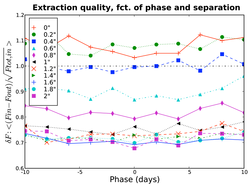
Figure 5: Same as Fig. 4 as a function of the phase of the simulated supernova

Note that the effect of the SN phase is very marginal (Fig. 5) , indicating that low contrast of the SN relative to the host is not critical to recover the SN spectrum. From inspection of the residuals, we find that the unaccounted curvature is the main source of contamination of the supernova spectrum by the host spectrum, which will scale with this contrast.

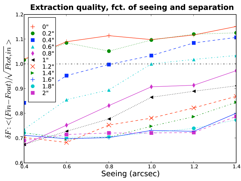
Figure 6: Same as Fig. 4 as a function of the seeing of the simulated VLT spectrum.

From Fig. 6, we see that for $d_{SN/Host\ centre}$ under 0.5^′′ and a seeing larger than 0.9^′′, $\delta F$ is above 1, but remains under 1.15 .

We conclude that in a wide range of redshifts, seeing and phases, PHASE efficiently recovers the fluxes of the SNLS VLT supernova spectra. At $z=0.5$ and for our median seeing of 0.7^′′, PHASE is able to extract separately the supernova from its host provided their separation is greater than $\sim 0.2^{\prime\prime}$ (1 pixel).

5 Results

5.1 Examples of PHASE extractions

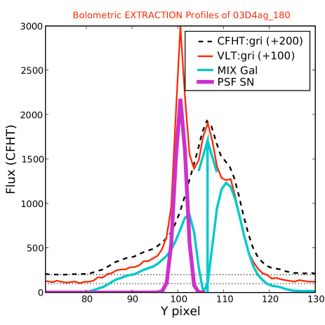
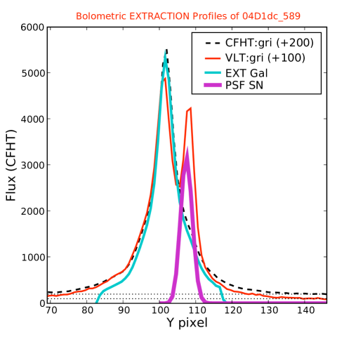
Figure 7: PHASE extraction “bolometric” profiles for SN 03D4ag (left) and SN 04D1dc (right). The case of SN 03D4ag illustrates a Mix host model composed of a Gaussian PSF core (represented as a blue arrow) and extended arms. The case of SN 04D1dc illustrates an EXT model. In both cases, the SN PSF model is represented as a magenta Gaussian. The horizontal dotted lines indicate the background level arbitrarily shifted for the sake of clarity.

In Fig. 7, we present two examples of PHASE models.

The left panel shows the “bolometric” profiles from the CFHT deep reference images (black dashed curve) and from the VLT LSS spectrum (red solid curve) of SN 03D4ag, an SN Ia at $z=0.285$ spectroscopically observed $\approx 9$ days before maximum light. The host is modelled as a Mix model (see Section 3.2.1) divided into a Gaussian core (represented by a blue arrow) and an extended asymmetric arm profile (blue solid line). The supernova is represented as a magenta Gaussian. We thus use a 3-component model (plus a uniform background component) to extract the spectrum of SN 03D4ag.

The right panel of Fig. 7 shows the same “bolometric” model in the simpler case of SN 04D1dc. Here, the host is an extended early spiral galaxy with no fine structure, in contrast to the host of SN 03D4ag. It is simply modelled by the profile measured on the CFHT deep reference image.

In both cases, a separate extraction of the supernova and the host is possible as their separation is above the default cut of 1 pixel ( $d_{SN/Host\ centre}$=1.09^′′ for SN 03D4ag and 1.18^′′ for SN 04D1dc).

After the spectra are extracted, the flux is corrected for exposure time, instrument response, atmospheric extinction – including absorption from molecular oxygen and water vapour. We also correct for slit losses under the assumption that the supernova is centred in the slit and that the PSF along the dispersion axis has the same properties as along the spatial axis (a Gaussian of FWHM equal to the effective seeing, with a wavelength variation following a power law of index -0.3). Note that no interpolation of contiguous pixel values is made, neither to filter cosmic hits, nor to re-sample the frames at uniform wavelength bins. This allows an accurate estimation of the noise level, and does not add any further correlation among pixels. One consequence of this procedure is that the extracted spectra have non-uniform wavelength bins.

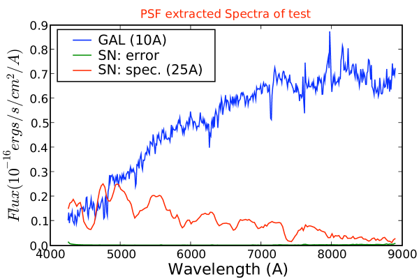
Figure 8: Top: PSF extracted spectra for SN 04D1dc. The host spectrum (blue line) has been rebinned with 10 $\AA$ while the SN (red line) spectrum is rebinned with 25 $\AA$. Spectra have been corrected for atmospheric absorptions and are presented in the observer frame. Bottom: extraction residual spectrogram. Position and profile inaccuracies are reflected in the residual spectrogram. Here, the supernova in the model is located $\sim 1$ pixel too close to the host centre. As a result, the model profile is not accurate: too much light is extracted at the centre and not enough on the edges. This yields negative residuals at the centre and positive residuals on the edges.

The top panel of Fig. 8 presents the extracted spectrum of SN 04D1dc (red line) along with its host galaxy (blue line). Spectra have been rebinned for visual convenience. The host spectrum exhibits the features of a typical early spiral (Sa/Sb) with [O ii], Ca H&K, H $\alpha$, N ii and S ii. Atmospheric absorption subtraction residuals are clearly seen, both in the host and the supernova spectra around 7600 $\AA$.

5.2 PHASE performances and limitations

In order to estimate its performances, we have applied PHASE to the extraction of all spectra of the ESO-VLT 1st large programme of the SNLS. The full results for the confirmed SNe Ia will be presented in Balland et al. (2008). A total of 829 LSS science and 2169 (896 MOS and 1273 LSS) calibration exposures have been processed to produce 208 calibrated spectrograms of SN candidates. In about 90% of cases, the default cuts yield an optimal extraction of the signal (including cases for which a separate extraction of the SN and host components was not possible), improved over standard extractions using classical techniques. The remaining 10% of cases are events for which extraction cuts are not suitable and thus the component definition is not adequate. These cases are tagged after inspection of the output spectrum and the residual spectrogram obtained in a first automatic extraction with default cuts. We treat these events on a case-by-case basis, adjusting the cuts to the specificity of the situation encountered.

PHASE performs the extraction of all the objects present in the slit. The supernova spectrum is extracted separately from the host whenever possible (about 70% of cases). Comparison to standard extractions (see Section 5.3) illustrates the efficiency of PHASE extraction within the limits of validity of the assumptions made. These latter include:

• that the coordinates of the supernova are accurate.

• that no flux from the supernova is present in the reference images.

• that the PSF is a Gaussian of width equal to the seeing.

• that the reference image seeing is equal or close enough to the combined spectrogram seeing.

Any deviation from these assumptions results in weak flux losses, higher noise and supernova spectrum contamination by its host. In particular, variation of the PSF with wavelength (other than the seeing dependence that we take into account) might be a concern. We have checked that our simple modelling of the PSF as a Gaussian profile yields an extraction within only a few percent of minimum variance. Thus, PHASE extractions are close to optimal.

In PHASE, the profile shape and centroïd must match as closely as possible those of the spectrogram. This means that one needs a deep reference image of seeing similar to the spectroscopic observation. However, the average seeing of the deep reference images is $1^{\prime\prime}$, while spectroscopic observations at Paranal have an average seeing of 0.8^′′. In this case, the exact shape of the source is not well reproduced by the Gaussian model (the galaxy is more peaked in the spectrogram than on the reference image). Position and profile inaccuracies are reflected in the residual spectrogram obtained when the extracted fluxes of all components are subtracted from the combined spectrogram. If the seeing of the reference image is higher than the one of the VLT spectrogram, the residuals are positive at the centre of the spectrogram and negative on the edges. Nevertheless, for a usual $0.1$ pixel position accuracy and a $0.1^{\prime\prime}$ seeing accuracy (of average $0.8^{\prime\prime}$), the flux loss amounts to $5\%$, with a noise increase of about $25\%$.

The bottom panel of Fig. 8 illustrates a situation for which the supernova coordinates are not accurate. Here, the Gaussian model for the supernova is located $\sim 1$ pixel too close to its host centre. The matching of the photometric profile to the spectroscopic profile yields too much light in the host model and not enough in the supernova, as can be seen in the right panel of Fig. 7. The extraction yields negative residuals at the centre and positive residuals on the edges.

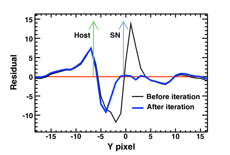
Figure 9: Average spatial profile of the residual spectrum before (black line) and after (thick blue line) PHASE iteration. Pixel 0 in the abscissa corresponds to the centre of the slit. Residual scale is in ADUs/pixel. The SN and host locations along the profile are indicated as vertical arrows. Only the position of the supernova component is allowed to vary during the iteration process.

In order to circumvent these limitations, the residuals can be used to iteratively adjust the position, slope and width of the SN component. The other (galactic) components can either stay fixed, or move together with the SN. Slope refinement applies to all sources and width refinement to point-like sources only. Iterating in this way yields an optimal extraction in a few passes. Figure 9 shows the improvement obtained after iterating in this way, in the case of SN 04D1dc. The black thin line is the average profile of the residual shown in the bottom panel of Fig. 8. The thick blue line is the average profile of the residuals after five iterations. The host position is kept fixed. At the end of the iterative process, the supernova position has moved by about one pixel and its width has decreased by $\sim 20$ %. Inspection of Fig. 9 shows that the residual flux of the supernova has disappeared after iteration. Although useful, we do not systematically iterate, for the sake of preserving an automatic extraction.

To improve further the residuals, one would need to refine the trace (i.e., use higher order polynomial coefficients) and PSF models (e.g., use Moffat functions for a better fit of the effects of seeing caused by atmospheric turbulence because of their longer tails).

Finally, regarding computer time costs, processing spectra with PHASE is rather efficient. Creating the master flat-field frame is the most time expensive task of the calibration stage. It takes about 5 minutes of CPU time on an Intel Celeron processor running CERN-Linux to perform an iterative median on 30 frames. The definition of photometric priors and the extraction stage in itself takes only a few seconds.

5.3 Comparison to standard extractions

In this Section, we compare PHASE and standard extractions on a few examples. Standard extractions have been performed using the Horne (1986) algorithm, in a way similar to what is done during the real-time processing of the SNLS-VLT spectra (Basa et al., 2008). With this method, the host and the supernova signals are often extracted together and the SN/host separation is done later when identifying the spectrum by adjusting a model built from template spectra. This model combines a fraction of supernova and a fraction of galaxy. From a purely practical point of view, using PHASE alleviates the user of a number of tasks such as the visual measure of the spatial shifts of the frames, the definition of the sky estimation regions, and the supernova and potential host extraction regions.

5.3.1 SN 03D4dy: a supernova resolved from its host

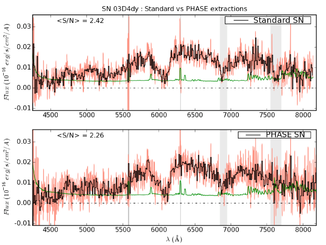
Figure 10: Comparison of standard (top) and PHASE (bottom) extractions for the simple case of SN 03D4dy, an SN Ia at $z=0.6$. Spectra have been rebinned with 10 $\AA$ (black) and are presented in the observer frame. The green spectra are the noise model for each extraction. The statistical noise is plotted in red. The grey lines correspond to the intense atmospheric O [i] emissions and the grey bands to atmospheric $O_{2}$ absorptions.

We compare here the spectra obtained with the standard and PHASE techniques, in the nearby subset of our sample, where the supernova is resolved from its host. This is the simplest possible situation and we expect that the two extraction methods yield comparable results. Figure 10 shows the two extractions for SN 03D4dy, an SN Ia at $z=0.6$. The standard extraction is shown in the top panel while the PHASE extraction is presented in the bottom panel. The green spectra are the noise model for each extraction. The host is not visible in the slit and the model is a simple PSF Gaussian of width equal to the seeing. As expected in this simple case, the two extractions yield comparable results in the whole spectral range. To further compare the two extracted spectra, we define the quantity $<S/N>$ as the signal-to-noise ratio per pixel, involving the statistical noise $N$ propagated during the processing (PHASE or standard) and averaged over all pixels. In the present example, we find that $<S/N>$ is slightly higher for the standard extraction ($<S/N>=2.42$) than for the PHASE extraction ($<S/N>$=2.26).

5.3.2 SN 03D4ag: a supernova in the arm of its spiral host

We consider here the case of SN 03D4ag, an SN Ia that exploded in the arm of a spiral galaxy at $z=0.285$. The definition of the sources is of critical importance in this case. In the standard procedure, two extractions are performed, one at the location of the supernova, the other in a region where the host signal is not contaminated by the SN. Then, this “pure” host spectrum is subtracted from the other to get the supernova spectrum. This subtraction affects the colour of the final supernova spectrum.

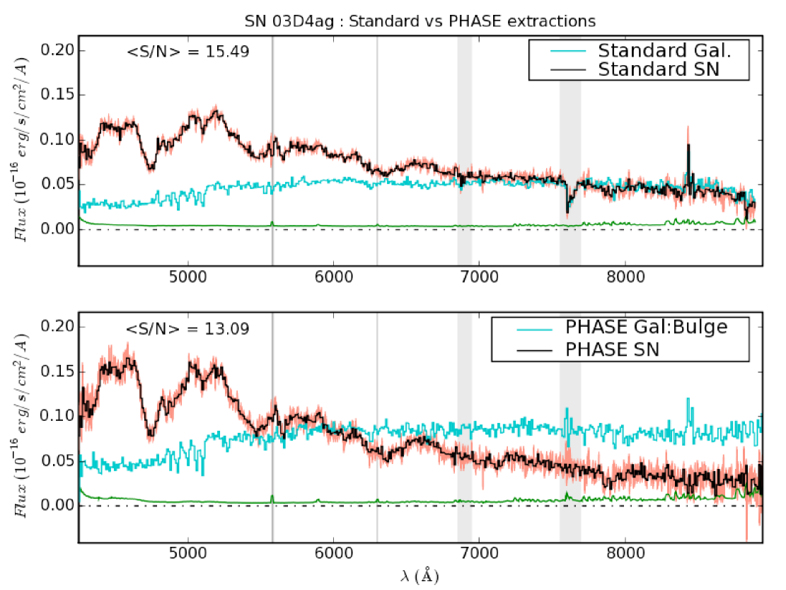
Figure 11: Same as Fig. 10 for SN 03D4ag, an SN Ia that exploded in the arm of a spiral galaxy at $z=0.285$. The Mix host model presented in the left panel of Fig. 7 is used to recover the different components. The PHASE supernova spectrum is bluer than the standard spectrum, as it should be for this $\phi\approx-8$ days SN Ia .

With PHASE, all sources are extracted at the same time provided that the sources are properly modelled. Figure 11 shows the comparison between the two extractions. The standard extraction limits the size of the extraction window to prevent from too high host contamination and only part of the SN flux is extracted. On the contrary, if the host is correctly modelled, PHASE assigns the correct flux to the supernova (see Section 4 above).

We find comparable $<S/N>$ for the two extractions (13.1 for PHASE and 15.5 for the standard extraction). The supernova spectrum extracted with PHASE is blue, consistent with its early phase ($\phi\approx$ -8 days). This is not the case for the standard spectrum that looks like an SN Ia spectrum around maximum light.

5.3.3 SN 04D2bt: a supernova close to its host centre

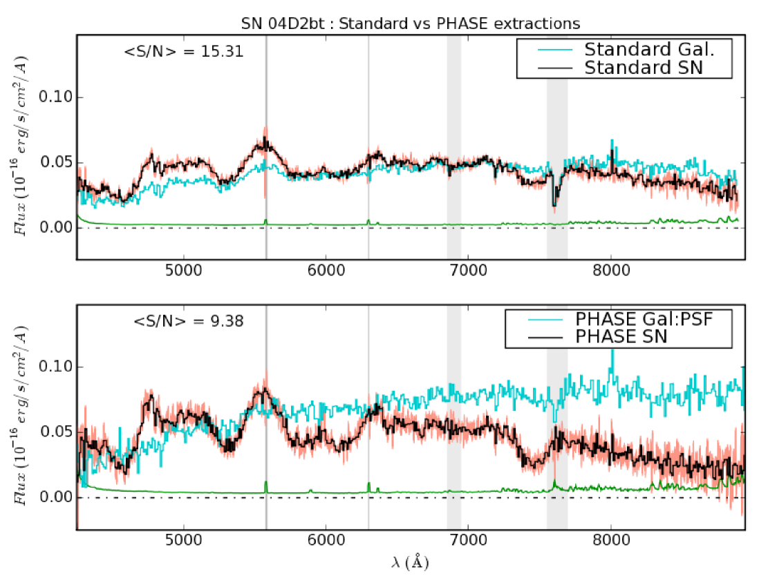
Figure 12: Same as Fig. 10 for SN 04D2bt, an SN Ia at $z=0.22$ that exploded very close to its host centre, which renders the component separation difficult. Here, a PSF model is used for the host and permits a clean restoration of the two components at the expense of a higher noise level.

SN 04D2bt is an SN Ia at $z=0.22$ that exploded very close to its host centre (0.35^′′ for a seeing of 0.62^′′). This renders the component separation difficult. Using a PSF model for the underlying galaxy, PHASE algorithm nevertheless succeeds in extracting separately the supernova and the host, as appears in Fig. 12. The host and supernova spectra obtained from the standard procedure are strongly correlated and the supernova flux is thus not accurate. With PHASE, both components are recovered correctly at the expense of a higher noise level.

6 Using SALT2 for the purpose of identifying SNLS spectra

In this Section, we turn to the identification of SNLS supernovae. Once an optimal spectrum of a potential supernova (sometimes combined with its host signal, see above) has been extracted using the PHASE extraction method, it is essential to assess the type of the candidate and to determine its redshift for the Hubble diagram.

6.1 Redshift determination

The redshift determination is based on the identification of a few galactic absorption or emission lines (e.g., [O ii], [O iii], Hydrogen Balmer series, Ca H&K, $4000\,\AA$ break). A Gaussian fit of one or more of these lines yields a typical uncertainty on the redshift of $\delta z\leq 0.001$ over the available spectral range. This is similar to the redshift determination accuracy obtained for similar spectral resolutions in Lidman et al. (2005); Hook et al. (2005); Howell et al. (2005); Balland et al. (2006, 2007).

The separate extraction of the host signal from the SN in a vast majority of cases simplifies galaxy line identification and redshift determination. However, in about 20% of cases, no host signal is visible at all and redshift determination has to be performed on SN features, from a series of fits of the supernova spectrum using the SALT2 model (Guy et al. 2007, see below). We allow the redshift to vary in a plausible range, given the supernova features, with a step of $\delta z=0.005$ and we determine the redshift from the best-fit solution. This latter determination yields a typical uncertainty of $\delta z\approx 0.01$, ten times larger than for an identification from host lines. This is in agreement with redshift determinations using correlation with a template, e.g. the SNID code developed by Blondin & Tonry (2007).

6.2 Identification

The identification proceeds in two steps:

1) We systematically perform a simultaneous fit of photometric (light curves) and spectroscopic data, using SALT2 with and without a galaxy template (see below). This yields a set of best-fit parameters whose values help at discriminating spectra with properties different from the average properties of the SALT2 SNe Ia training set (Guy et al., 2007).

2) We then decide the type of the spectrum. This step is not automatic. We use both visual inspection of the fitted spectrum and the parameter values of the best-fit SALT2 model. The final decision is based on qualitative grounds. Nevertheless, using the SALT2 fit greatly helps in discriminating SNe Ia from other types, as both spectroscopic and photometric fit parameters are different for the two. In particular, we know the date of maximum, and thus the phase. Using the SALT2 fit allows us to alleviate the phase degeneracy between SNe Ia and SNe Ic (see below).

In the following, we detail these two steps.

The spectrophotometric template SALT2 (Guy et al., 2007) has been designed to fit the light curves of observed supernovae. As it is trained against a whole set of SNe Ia spectra templates, including both local, published SNe Ia templates and more distant SNe Ia spectra, including 39 SNLS first year spectra both from the VLT (Balland et al., 2008) and Gemini (Howell et al., 2005) telescopes, it is possible to use it for a combined fit of the photometric data and the spectrum of a given supernova. This procedure has been briefly discussed in Guy et al. (2007) and is extensively used in the present work. It offers the great advantage over a simple spectral fitting as the ones used in a lot of previous works concerned with SNe Ia spectral identification (Lidman et al., 2005; Matheson et al., 2005; Foley et al., 2008; Balland et al., 2006, 2007; Hook et al., 2005; Howell et al., 2005; Wood-Vasey et al., 2007) to explicitly incorporate, in the spectral identification process, information on the date of B-band maximum light and colour. This, in particular, alleviates the possibility of confusing a Type Ib/c supernova (SN Ib/c) with an SN Ia, at least at early phases, and has yielded, in several cases, a firm type determination of dubious spectra. It is also a good way to discriminate Branch-normal SNe Ia (Branch et al., 1993, 2006) from more peculiar objects for which SALT2 fails at providing a satisfying spectrophotometric model.

The identification using SALT2 is based on a $\chi^{2}$ minimisation procedure from the combined fitting of photometric and spectral data for a given supernova. The main photometric parameters entering the fit are the principal components $x_{0}$, $x_{1}$ of the SALT2 model (see Guy et al. 2007 for details) and the colour index $c$, defined as the difference between $(B-V)_{SN}$ and the average $<B-V>$ value for the whole training sample. The colour law of the model is obtained during the training process on the SALT2 training sample, along with the model components (see Fig. 3 of Guy et al. 2007 for a comparison to a Cardelli et al. 1989 law). The $x_{1}$ parameter is linked to the stretch of the supernova and can be interpreted as the number of standard deviations the stretch of the supernova under study is with respect to the whole training set. A set of spectroscopic parameters are fitted along with the photometric parameters and include a possible host fraction, an overall normalisation parameter and a tilt parameter. These two latter parameters allow us to take into account possible errors in the flux calibration, due to, e.g., variations from the time average response function used for flux calibration, or differential refraction effects improperly corrected for. Higher order re-calibration parameters can be added at will, but we usually limit the possibility of spectral re-calibration to the two parameters described above, except for high S/N spectra, for which adding a third re-calibration parameter improves the overall fit by also correcting for “curvature” effect along the spectrum.

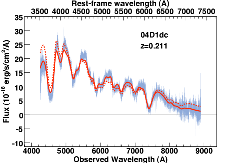
Figure 13: SALT2 fit of SN 04D1dc, an SN Ia spectroscopically observed at maximum light. Top: negative deep reference image of SN 04D1dc host. The locus of the SN explosion is indicated with a “+” sign. The position of the slit is shown as green dotted lines. Bottom left: restframe $g_{M}$,$r_{M}$,$i_{M}$,$z_{M}$ light curves and corresponding SALT2 fits. Bottom right: PHASE extracted spectrum with the best-fit SALT2 model overlapped. Dashed red line is the raw SALT2 model. Solid line shows the best-fit model after re-calibration using 3 parameters. The spectrum is presented in the observer frame and the restframe wavelength is reported on top.

Figure 13 presents an example of the combined identification performed with SALT2. Recall that SN 04D1dc is an SN Ia at maximum light at $z=0.211$, well separated from its host core (see top panel of Fig. 13). A separate PHASE extraction of the host and the supernova was possible, yielding an almost host-free supernova spectrum (Section 5.1 and Fig. 8). The bottom left panel of Fig. 13 shows the $g_{M}$, $r_{M}$, $i_{M}$, and $z_{M}$ photometric data, along with the best-fit SALT2 light curves models overlapped. The fit is excellent in each band and the secondary maxima, typical of SNe Ia, are clearly seen in the infrared light curves. The bottom right panel of Fig. 13 shows the corresponding spectral fit. The dashed red line is the SALT2 model obtained with no re-calibration, the solid red line being the same model but with re-calibration (using three re-calibration parameters in this specific case). In this example, re-calibration appears to have a weak effect on the final fit (significant only around 4000-4500 $\AA$). This indicates that flux calibration is accurate. Strong discrepancies between the dashed and solid red lines appear in some cases, hinting either towards a problem in flux calibration, or, more probably, an inadequacy of the model to reproduce the spectral data. This happens in particular for spectra of supernovae that cannot be adequately reproduced by SALT2 (such as SNe Ic) as only SNe Ia are considered in the SALT2 training sample.

When it was not possible to extract separately the supernova from the host signal with PHASE, the SALT2 fit incorporates a galaxy template in the model (Guy et al., 2007). We use galaxy spectral series synthesised by PEGASE2 (Fioc & Rocca-Volmerange, 1997, 1999) for various Hubble types (Elliptical, S0, Sa, Sb, Sbc, Sc and Sd). Each series ranges from 1 Gyr to 13 Gyrs and offers a continuous sequence from blue to red within each Hubble type. We also use the spectral templates for Elliptical, S0, Sa, Sb and Sc types from Kinney et al. (1996). The best-fit interpolated galaxy template and age are obtained as part of the minimising procedure.

We have checked the quality of PHASE SN/Host separation. To do this, we have selected all the SNe Ia of the 1st VLT large programme for which a separate extraction of the SN component from its host was possible. We then did a SALT2 fit of these supernovae with a galactic component in the fitted model. For this specific test, we only used the Kinney et al. (1996) Hubble sequence (from Elliptical to Sc types). We discarded four extinguished supernovae with very red colours and two supernovae for which no acceptable fit was obtained. We ended up with a sample of 68 SNe Ia (among which 47 were identified as certain SNe Ia, see our classification definition below). With the whole sample, we find that the average galaxy fraction in the best-fit model is $4.5\pm 3.0$ % with a dispersion of 25%. If we restrict ourselves to the sample of 47 certain SNe Ia, we find an average galaxy fraction of $0.7\pm 3.2$ % and the dispersion slightly decreases to 22 %. These results confirm that residual host light contamination of the PHASE extracted supernovae is moderate.

For each SNLS supernova for which both photometric data (in at least two bands) and a spectrum are available, we perform SALT2 fits using all galaxy types with two re-calibration parameters. Light curves are fitted in the range -15 and +40 days, which turns out to be sufficient for most supernovae under investigation. Spectra are fitted over their whole spectral range. The best-fitting model is for the minimum combined (photometric and spectral) $\chi^{2}$ value. Result parameters and fits are inspected to assess the identification of the candidate as a SN Ia (step 2 of our identification process). Large $x_{1}$ absolute values hint possible peculiarities (under or over-luminous SN). Large positive colour indexes are either due to large intrinsic or galactic reddenings, or possible SN Ib/c. Large negative values are found for Type II supernovae (SN II), for which no good spectral fits are obtained. Light curves and spectral fits are visually inspected. When strong re-calibration is necessary to obtain a good spectral fit, we track down the reason for this. Often, this is the sign of a non SN Ia spectrum. The combination of all these indicators usually leads to an optimised identification, even though the final decision relies on human judgement.

Spectra of SNe Ia are classified according to the following scheme: SN Ia (certain SN Ia), SN Ia$\star$ (possible SN Ia but other types, in particular SN Ic, cannot be excluded given the S/N and phase), SN Ia_pec (peculiar SN Ia), SN (certain SN as the spectrophotometric properties match the known properties of an SN although the type is not clear), SN? (possible SN of unclear type, other objects such as variable stars or AGNs are possible), SN Ib/c, SN II. Note that this classification scheme slightly differs from the classification adopted in Astier et al. (2006). The Hubble diagram is built only from SN Ia and SN Ia$\star$ supernovae or from SN Ia supernovae alone, underlying the necessity for a clean supernova identification.

6.3 Results of the identification

In this Section, we illustrate the performances of our SALT2-based identification through a series of representative examples. The bulk of our SNe Ia identifications will be published in Balland et al. (2008). In the examples given below, we show the results of the spectral and light curve fits for the sake of completeness. Spectra are presented in the observer frame and the restframe wavelength is reported on top of the corresponding Figure. The SALT2 model output parameters are summarised for each example in Table PHotometry Assisted Spectral Extraction (PHASE) and identification of SNLS supernovae.

6.3.1 SN 05D2dt: a high S/N SN Ia at $z\sim 0.6$

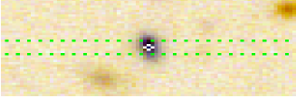
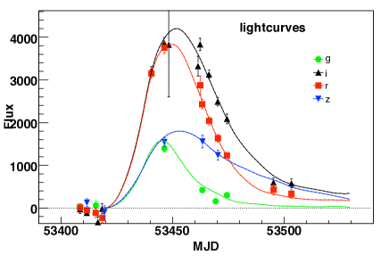
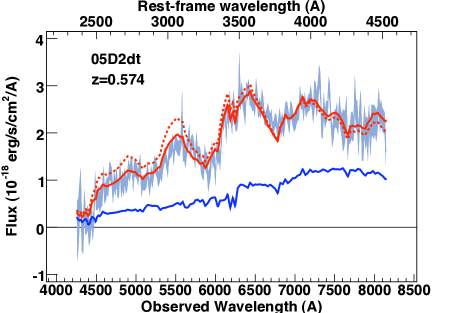
Figure 14: SALT2 fit of SN 05D2dt. Top left: negative deep reference image of SN 05D2dt. The locus of the SN is indicated as a “+” sign. The slit position is shown as green dotted lines. Top right: restframe $g_{M}$,$r_{M}$,$i_{M}$,$z_{M}$ light curves and corresponding SALT2 fits. Bottom left: full PHASE extracted spectrum (including host signal) with SALT2 raw (dashed line) and re-calibrated (solid line) models. For the latter, two re-calibration parameters have been used. Bottom right: host-subtracted spectrum with SALT2 best-fit model overlapped. The spectra have been rebinned to 15 Å. This supernova is identified as an SN Ia.

In Fig. 13, we have shown the case of a host free, low-redshift SN Ia at maximum light. Figure 14 shows the spectrum of SN 05D2dt, a $\phi\approx-2$ days SN Ia at $z=0.574$ (about the average redshift of the SNLS sample), observed at the VLT. This supernova lies at the centre of its host (see top left panel of Fig. 14) and no separate extraction was possible. The bottom left panel of Fig. 14 shows the full, host-contaminated spectrum and the SALT2 best-fit model (before and after re-calibration). The bottom right panel shows the host-subtracted spectrum, with the calibrated model overlapped. In both cases, the spectrum has been rebinned with 15 $\AA$ bins for the sake of visual convenience. In the bottom left panel, the model galaxy is plotted as a blue solid line. Contribution of the host model to the full model is computed in each photometric band. A “bolometric” fraction of host is also evaluated over the full available spectral range and is given in Tab. PHotometry Assisted Spectral Extraction (PHASE) and identification of SNLS supernovae. In the case of SN 05D2dt, a fair host contamination ($43\%$ of host template in the fitting model) is present and is well modelled by an early-type template. The model is tilted in order to adequately reproduce the spectrum, but this re-calibration is only moderate ($\approx 10$ % flux re-calibration from $\lambda=4500$ Å  to $\lambda=8500$ $\AA$). Once the host contribution has been subtracted, the SNe Ia features are very well reproduced by the SALT2 model (bottom right panel of Fig. 14) and the identification as an SN Ia is unambiguous at this phase, even if no clear Si ii can be seen around restframe 4000 $\AA\$ due to the S/N level.

6.3.2 SN 04D4ib: an SN Ia buried into its host signal

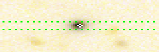
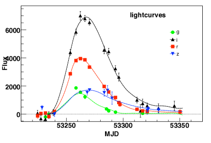
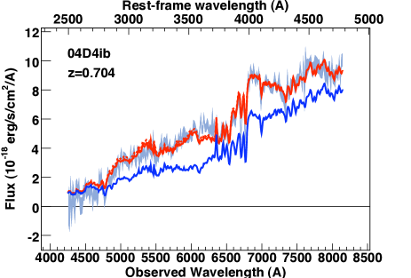
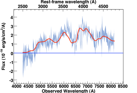
Figure 15: Same as Fig. 14 for SN 04D4ib. This supernova is identified as an SN Ia.

We show here SN 04D4ib, an SN Ia at $z=0.704$ deeply contaminated by its host core signal. This is a “SNGAL” case, for which PHASE cannot extract separately the supernova and the host. Figure 15 shows that the SALT2 fit is efficient at recovering the supernova spectrum (bottom right panel) from the full, host contaminated spectrum (bottom left panel). Here, a fraction of 71% of a Kinney et al. (1996) S0 template has been subtracted. Host Ca ii lines subtraction residuals are clearly seen in the supernova spectrum, but the broad SN features are well reproduced by the fit. No Si ii at 4000 Å  is visible, but given the phase of this SN ($\phi=+1$ day), confusion with an SN Ic is unlikely (see below Section 6.3.4) and we can secure the type as an SN Ia.

6.3.3 SN 04D4dw: a distant ($z\sim 1$) SN Ia$\star$

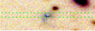
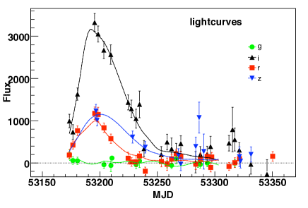
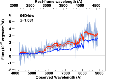
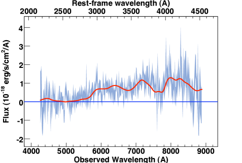
Figure 16: Same as Fig. 14 for SN 04D4dw. This supernova is identified as an SN Ia$\star$.

SN 04D4dw at $z=1.031$ is the second farthest SN Ia of the 3rd year SNLS sample. This is another “SNGAL” case for which PHASE is not able to efficiently perform a separate extraction. Figure 16 shows the full spectrum (bottom left panel) and host-subtracted supernova spectrum (bottom right panel). Due to its high redshift, the UV part of the spectrum is visible down to restframe 2100 Å  and is correctly reproduced by the SALT2 fit. This is not an obvious result, as the SALT2 training sample is rather poor in UV spectra (Guy et al., 2007). The redshift is obtained from the presence of Ca ii absorption lines. The blueshifted Ca ii around restframe 3700 Å  and possibly some Si ii at restframe 4000 Å  are visible in the spectrum of this supernova slightly past maximum ($\phi=2.1$ days). Given the rather low S/N, it is identified as an SN Ia$\star$.

6.3.4 SN 04D4jv: an SN Ic supernova

The possible confusion of an SN Ia with an SN Ic is a concern when identifying a supernova candidate. Indeed, the spectral structure of an SN Ia slightly past maximum light resembles the one of an SN Ic a few days before maximum (compare for instance the spectra of SN 2002bo, Benetti et al. 2004, 4 days past maximum and of SN 1994I, Filippenko et al. 1995, 5 days before maximum). This degeneracy is amplified at larger redshift, as the spectral range of the observed spectrum and the S/N decrease with redshift and it is often difficult to confidently rule out the possibility of an SN Ic. Using SALT2 for the purpose of identification alleviates this degeneracy, as the phase is in principle known from the light curve fitting. The fact that SALT2 fails at reproducing a spectrum is in itself an indication that it is unlikely to be an SN Ia, as far as the phase and spectral coverage are well described by the SALT2 training set. Moreover, the values of the SALT2 colour value $c$ might also help, as SNe Ic are redder than SNe Ia at the same phase. Indeed, SNe Ic tend to have high colour values, $c\geq 0.3$ (even if this sole result is not sufficient to unambiguously classify a supernova as an SNe Ic, as very extinguished SNe Ia would have comparable $c$ values). Nevertheless, it has been noted that SNe Ic and SNe Ia spectra show the greatest similarity about one week after maximum light (Hook et al., 2005; Howell et al., 2005). In particular, iron absorption features are present in SNe Ic spectra in the range $4200-5000$ Å, that resemble the spectral shape of SNe Ia $\sim$ 1-2 weeks after maximum light. Identification of later-phase spectra thus remains subject to caution, especially given the S/N of SNLS spectra at $z\sim 0.5$. A substantial fraction of supernovae classified as SN Ia$\star$ in our sample correspond to this situation of a $\sim 1$ week past maximum SN, for which a fair SN Ia match is obtained with SALT2 but an SN Ic solution cannot be confidently ruled out. The remaining SN Ia$\star$ are usually due to low S/N.

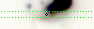
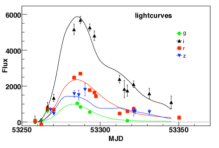
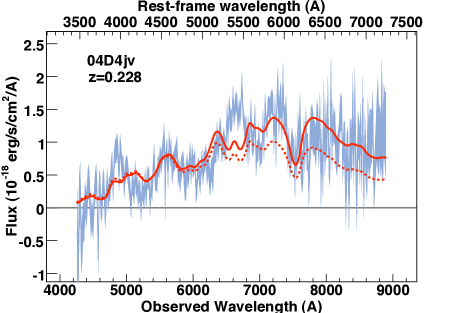
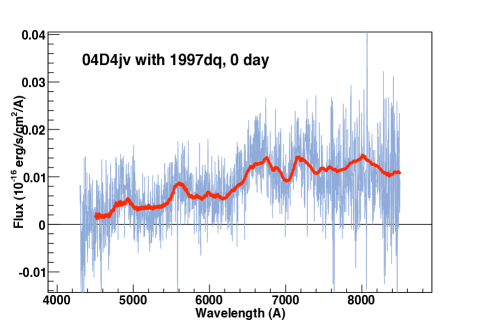
Figure 17: SALT2 fit of SN 04D4jv. Top left: negative deep reference image of SN 04D4jv. The locus of the SN is indicated as a “+” sign. The slit position is shown as green dotted lines. Top right: restframe $g_{M},r_{M},i_{M},z_{M}$ light curves and corresponding SALT2 fits. Bottom left: PHASE extracted spectrum with SALT2 raw (dashed line) and re-calibrated (solid line) models. Even with strong re-calibration, SALT2 fails at correctly reproducing the spectrum around 6500 Å. Bottom right panel shows a fit of SN 04D4jv with an SN Ic template (SN 1997dq at maximum light, Matheson et al. 2001) obtained using the ${\cal SN}$-fit software (see text). The spectrum in the right bottom panel is not rebinned. This supernova is identified as an SN Ic.

The bottom left panel of Fig. 17 shows the best SALT2 match of SN 04D4jv (light curves and spectrum), an SN Ic at $z=0.228$ around maximum. If the light curve fit is visually acceptable, the SALT2 colour index is however very high: $c$=0.96 (see Tab. PHotometry Assisted Spectral Extraction (PHASE) and identification of SNLS supernovae; by construction the average $c$ of the SALT2 training sample is 0). SALT2 clearly fails at reproducing the SN structure seen in the spectrum around 4800 Å  and between 6200 and 7000 Å, even with strong re-calibration allowed (compare the dashed and solid lines). A good match with an SN Ic template (SN 1997dq at maximum light, Matheson et al. 2001) is obtained using the ${\cal SN}$-fit software (see Section 2.1) and is shown on the bottom right panel of Fig. 17. This confirms that SN 04D4jv is an SN Ic.

6.3.5 SN 05D4ar: an SN II supernova

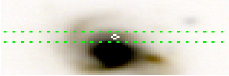
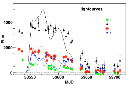
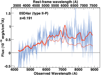
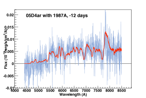
Figure 18: SALT2 fit of SN 05D4ar. Top left: negative deep reference image of SN 05D4ar. The locus of the SN is indicated as a “+” sign. The slit position is shown as green dotted lines. Top right: restframe $g_{M},r_{M},i_{M},z_{M}$ light curves and corresponding SALT2 fits. SALT2 does not correctly fits these flat light curves. Bottom left: PHASE extracted spectrum with SALT2 raw (dashed line) and re-calibrated (solid line) models. Even with strong re-calibration, SALT2 fails at correctly reproducing the spectrum, namely the $H_{\alpha}$ P-Cygni feature at 7900 $\AA$ (observer frame). Bottom right panel shows a fit of SN 05D4ar with an SN II template (SN 1987A, $\phi=-12$ days, Pun et al. 1995) obtained using the ${\cal SN}$-fit software (see text). The spectrum in the right bottom panel is not rebinned. This supernova is identified as an SN II.

In a similar way, we identify SN 05D4ar as an SN II (Fig. 18). Here, both the light curve and spectrum SALT2 fits are very poor. Both $x_{1}$ and $c$ are very discrepant from the average values of the training sample: $x_{1}=5$ and $c=1.29$, see Tab. PHotometry Assisted Spectral Extraction (PHASE) and identification of SNLS supernovae. The bottom right panel shows the fit obtained with ${\cal SN}$-fit using SN II templates. The best-fit is for SN 1987A a few days after explosion (-12 days with respect to maximum light, Pun et al. 1995). The H$\alpha$ P-Cygni emission is well reproduced, as are most of the noticeable features of the spectrum. Combined to the obvious flatness of the light curves, this fact confirms that SN 05D4ar is an SN II supernova.

7 Discussion

We have taken advantage of SNLS having two independent pipelines to cross-check the identifications obtained using SALT2 with the ones done with more standard procedures of template fitting. For a given object, an independent assessment of the type and the redshift was performed on each side. On one side, the superfit code developed by Howell et al. (2005) was run on PHASE extracted spectra, using all possible SN type templates. On the other side, SALT2 was systematically run on all PHASE spectra. Putting our efforts together, we have thus carefully double-checked the identifications of a sample of about 250 VLT, Gemini and Keck spectra. For VLT spectra, both extraction with PHASE and identification with SALT2 considerably improve the type determination. For Gemini spectra, not currently supported in PHASE, we only test the effect of using SALT2 as opposed to standard template fitting techniques. SALT2 identifications are straightforward and help in many cases to secure the type of the SN candidate. In some cases, the template fitting technique does a better job at reproducing the candidate spectrum. This usually happens for rather peculiar spectra not well represented in the SALT2 training sample. A few supernovae that had not been identified previously and that had been consequently classified as unknown objects, have proved to be SNe Ia in the light of our refined procedure.

Identifications based on the $\chi^{2}$ fitting of the SN spectrum against a host and an SN template library (Balland et al., 2006, 2007; Howell et al., 2005; Lidman et al., 2005) improve over the traditional eye-guided identification of “typical” SNe Ia features. However, they rely on the template library quality that often suffers from insufficient phase and wavelength coverage and/or completeness, especially for non SNe Ia templates. Cross-correlation techniques used by ESSENCE (Matheson et al., 2005) and SDSS (Zheng et al., 2008), though sophisticated, suffer to some extent from the same drawbacks, as they also rely on the comparison to a spectral external template dataset. Blondin & Tonry (2007) show that the SNID code is able to confidently distinguish an SN Ic at redshift 0.5 with phase between -5 and + 5 days from other SN types, depending on the use of priors on the redshift and age (see Fig. 21 of Blondin & Tonry (2007) for details). However, this method has the limitation that it can not subtract host galaxy.

Using SALT2 takes advantage of the spectrophotometric model of SNe Ia built from a large collection of spectra and light curves of local and distant SNe Ia, a fraction of which being SNLS supernovae. One of the key advantages of SALT2 is that the model improves as more SNe Ia are detected and identified as part of SNLS and external collaboration efforts. Moreover, using simultaneous photometric and spectroscopic information narrows the parameter space available to reproduce the SN properties. As an example, with SALT2, the phase is well constrained to within a fraction of a day, which allows us to alleviate the possible confusion with other types, such as SNe Ic. Non SNe Ia events are detected, as they produce parameters values or fits that deviate from the ones of the average sample. As a model is compared to the light curves and spectral data, the limitation due to incomplete spectral and phase sampling is not as strong as in the standard template fitting technique. All supernova candidates are treated on an equal footing and using SALT2 limits the subjective part of the identification introduced by human judgement. If SALT2 helps at discriminating non SNe Ia candidates, the current version of the code does not help in identifying their type. For such cases, recourse to a standard template fitting technique is required to secure the type.

8 Conclusion

We have developed new techniques for both supernova spectral extraction and identification. These new tools have been developed for the purpose of making use of the deep imaging obtained at CFHT to obtain an homogeneous set of SNLS supernova spectra.

Considerable effort has been put into extracting, in the most efficient way, VLT spectra in order to get a clean set of supernova spectra at redshifts ranging from $z=0.1$ to $z\approx 1$. One key feature of our so-called PHASE extraction is that the extraction is guided by computing the trace of the supernova on the spectrogram. This is done by using deep CHTLS reference images, in various photometric bands, to recover the profile of the non-transient objects present in the slit, from which a multi-component model is built by adding the (point-like) supernova flux as a Gaussian of width equal to the seeing. Fitting the model to the spectrogram light yields the flux of each component in each pixel. As we have shown, this improves the host-supernova separation over more standard techniques. A second key feature of the PHASE extraction is that it avoids re-sampling the data and correlating pixels along the procedure. This ensures a clean estimation of the error level associated with the signal used later for the identification.

We use the spectrophotometric model of SALT2 (Guy et al., 2007) as an help to determine the type of supernova candidates. Taking advantage of an ever increasing training set as new supernovae are discovered and followed up by the SNLS and other collaborations, the model is able to adequately reproduce SN Ia features in a wide range of cases (Balland et al. 2008 show that it is true from phases as early as -10,-15 days up to a few weeks after maximum light and for a wide spectral range, including the UV region down to 2100 $\AA$ for the most distant supernovae). The combined fit of light curves and spectrum tightens the constraints on the parameters that describe the supernova. Non SNe Ia candidates are identified on a case-by-case basis as their spectrophotometric best-fitting parameters deviate from the average properties of the SNe Ia training sample. Uncertainty however remains for the most host-contaminated (host fraction $>$ 70-80%) and most distant ($z\stackrel{{\scriptstyle>}}{{{}_{\sim}}}1$) cases.

PHASE extractions have been tested against simulations, and SALT2 based identifications have been cross-checked with template fitting identifications performed on the VLT data using the technique described in Howell et al. (2005).

We find that using SALT2 for the purpose of identification improves the reliability of the type determination over standard techniques. For VLT spectra, PHASE extraction combined to SALT2 identification takes the most possible out of the data to secure a clean type and redshift determination.

[c]lccc—ccccc Results of SALT2 fits used as an help for identification

SN SALT2 model
———————————————————— ——————————————————–
Name $z$ Phase (days/max) $d_{SN-Host\ centre}^{a}$ $x_{1}^{b}$ $c^{b}$ Host Model % host^c $\chi^{2}$/d.o.f.

04D1dc 0.211 -0.4 1.18 -1.56 0.01 NoGalaxy^d 0 3.24
05D2dt 0.574 -1.7 0.01 0.01 0.08 E 43 1.13
04D4ib 0.704 0.7 0.18 0.60 -0.10 S0 71 0.61
04D4dw 1.031 2.1 0.11 1.35 0.02 Sa 68 1.03
04D4jv 0.228 -1 1.5 -0.30 0.96 NoGalaxy^d 0 1.43
05D4ar 0.191 1.3 0.7 5.00 1.29 NoGalaxy^d 0 1.71

^a Distance (in arcsec) of the supernova centre to its host centre in the PHASE extraction model.

^b From the SALT2 fit of the light curves.

^c Percentage of host signal in the best-fitting model, averaged over the whole spectral range.

^d The best-fitting SALT2 model has no host component.