Magneto-thermal properties of the spin-$s$ Heisenberg antiferromagnet on the cuboctahedron

Abstract

We use the example of the cuboctahedron, a highly frustrated molecule with 12 sites, to study the approach to the classical limit. We compute magnetic susceptibility, specific heat, and magnetic cooling rate at high magnetic fields and low temperatures for different spin quantum numbers $s$. Remarkably big deviations of these quantities from their classical counterparts are observed even for values of $s$ which are usually considered to be almost classical.

1 Introduction

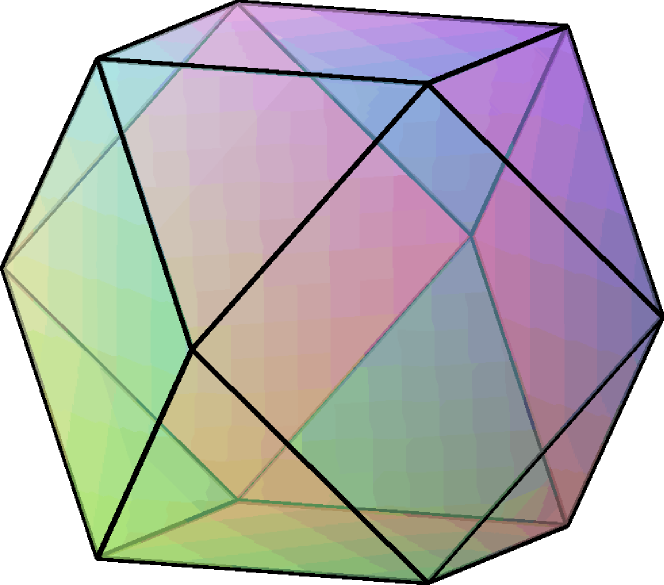
Figure 1: The cuboctahedron: a highly frustrated magnetic molecule with 12 spin sites.

Efficient low-temperature cooling by adiabatic demagnetization is a potential application of highly frustrated antiferromagnets [1, 2, 3, 4, 5]. However, quantitative theoretical results for the magneto-thermal properties have so far been obtained only in the classical case [1, 2] and the extreme quantum case of spin $s=1/2$ [3, 4, 5], with the exception of a study of the magnetocaloric effect in a (non-frustrated) ferrimagnetic spin-$(5/2,1)$ chain [6]. Note that numerical computations are already quite demanding for highly frustrated spin-1/2 antiferromagnets in low dimensions and become quickly unfeasible for $s>1/2$ or in higher dimensions.

The cuboctahedron (see Fig. 1) is a highly frustrated molecule which can be considered as a variant of the kagome lattice with 12 sites. At high magnetic fields, it supports localized magnon excitations [7, 8] which can be understood to be responsible for the enhanced magnetocaloric effect in these frustrated quantum spin systems. Several works have used the cuboctahedron as a model system for studying magneto-thermal properties [9, 10, 11]. Here we continue along these lines and use the cuboctahedron to investigate the behavior as a function of the spin quantum number $s$.

2 Model, observables and method

We consider the Heisenberg antiferromagnet in an external magnetic field $h$

$$H=J\sum_{\langle i,j\rangle}\vec{S}_{i}\cdot\vec{S}_{j}-h\sum_{i}S_{i}^{z}\,,$$ (1)

where the $\vec{S}_{i}$ are quantum spin-$s$ operators and $J>0$ is the exchange constant between nearest neighbor sites $\langle i,j\rangle$. The classical Heisenberg model is obtained from (1) in the limit $s\to\infty$ at fixed $J_{\rm cl}=s^{2}\,J$, $h_{\rm cl}=s\,h$. In this classical limit the operators $\vec{S}_{i}$ can be considered as unit vectors. Accordingly, a thermodynamic quantity ${\cal Q}_{s}$ for quantum spin $s$ approaches the classical limit as

$$s^{\alpha_{\cal Q}}\,{\cal Q}_{s}\left(\frac{T}{s^{2}\,J},\frac{h}{s\,J}\right)\ \mathop{\longrightarrow}_{s\to\infty}\ {\cal Q}_{\rm cl.}\left(\frac{T}{J_{\rm cl}},\frac{h_{\rm cl}}{J_{\rm cl}}\right)\,.$$ (2)

Using their definitions, it is easy to show that $\alpha_{\chi}=0=\alpha_{C}$, $\alpha_{M}=-1$, and $\alpha_{\Gamma_{h}}=1$, where $\chi$, $C$, and $M$ are the magnetic susceptibility, specific heat, and magnetization, respectively. Due to the discrete level spacing, quantum effects will be important below a crossover scale $E_{\rm q}\propto s\,J$, i.e., for $T\lesssim E_{\rm q}$. At temperatures $T\gtrsim E_{\rm q}$, ${\cal Q}_{\rm cl.}$ is expected to yield an approximation to ${\cal Q}_{s}$ after rescaling according to Eq. (2). The absolute value of the crossover scale $E_{\rm q}$ is unknown, but one may hope that it is small in highly frustrated magnets because of the generic reduction of energy scales.

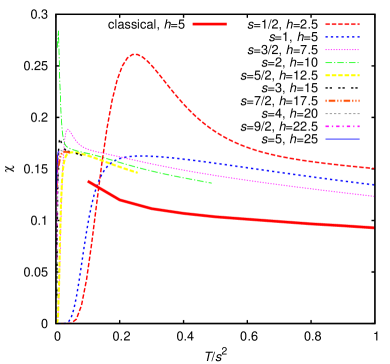
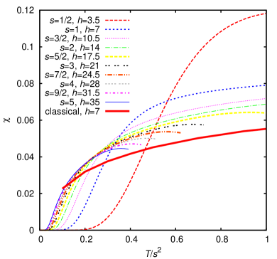
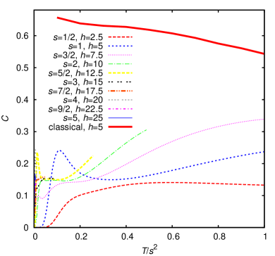
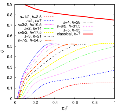
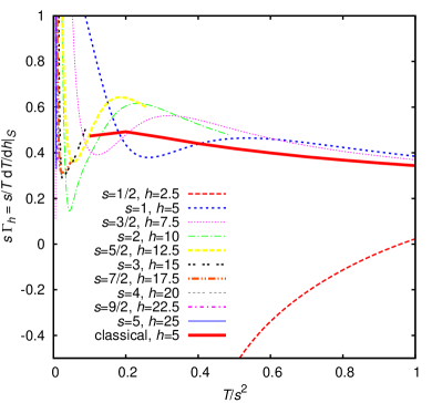
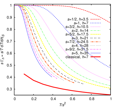
Figure 2: Magneto-thermal properties slightly below (left column) and slightly above (right column) the saturation field: magnetic susceptibility (top), specific heat (middle), and cooling rate $\Gamma_{h}$ (bottom). All quantities are normalized to the number of spins (12).

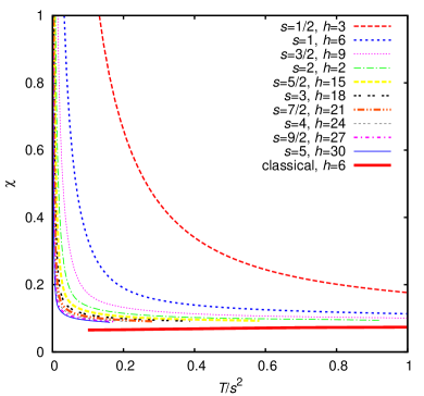
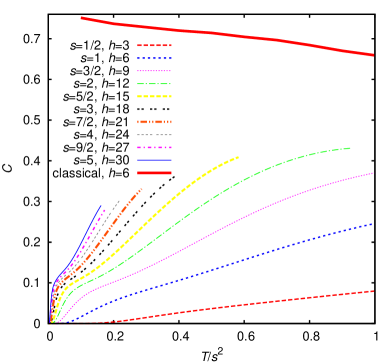
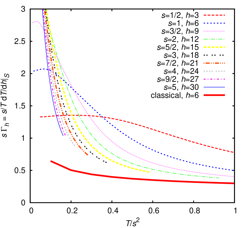
Figure 3: Magneto-thermal properties exactly at the saturation field: magnetic susceptibility (top, left), specific heat (top, right), and cooling rate $\Gamma_{h}$ (right). All quantities are normalized to the number of spins (12).

We will be particularly interested in the adiabatic cooling rate at fixed entropy $S$

$$\Gamma_{h}=\frac{1}{T}\,\left.\frac{{\rm d}T}{{\rm d}h}\right|_{S}=-\frac{1}{C}\,\left.\frac{{\rm d}M}{{\rm d}T}\right|_{h}\,.$$ (3)

Thermodynamic quantities can be computed for the cuboctahedron by full diagonalization for $s=1/2$ and $1$. For $s\geq 3/2$ we have to resort to a truncation of the spectra to low energies and one should be careful about truncation artifacts. Therefore we consider only temperatures $T\lesssim E_{\rm c}/10$ if the spectrum is complete until an excitation energy $E_{\rm c}$ even if we have partial results also for higher energies. For the classical case we use a combination of the Metropolis Monte Carlo algorithm with over-relaxation steps.

3 Results

Now we present some results for the low-temperature region $T\leq s^{2}\,J$, choosing $J=1=J_{\rm cl}$ for simplicity. The behavior close to the saturation field $h=6\,s$ is shown Figs. 2 and 3. We can see a trend of convergence towards the classical limit, in particular in the cooling rate $\Gamma_{H}$. However, quantitative corrections remain large for most cases, even for spin quantum numbers which are as big as $s=5$. The least systematic behavior at low temperatures is seen in Fig. 2 for $h=5\,s$ where the system becomes gapless in the limit $s\to\infty$. A gap opens above the saturation field which leads to the thermal activation of $\chi$ and $C$ observed in Fig. 2 for $h=7\,s$. Exactly at the saturation field, a total of 9 states with different magnetic quantum numbers becomes degenerate at $T=0$ [7, 10, 11]. This leads to the $1/T$ singularity in $\chi$ and the big values of the cooling rate $\Gamma_{h}$ which can be observed in Fig. 3. For $s=1/2$ and $h=3$ we reproduce previous results for the specific heat $C$ [9]. Both the thermal activation at $h=7\,s$ as well as the $1/T$ singularity in $\chi$ at $h=6\,s$ are quantum effects which disappear in the classical limit.

4 Discussion

Remarkably big deviations from the classical behavior are observed for magneto-thermal properties of the cuboctahedron with $s\leq 5$. This should not come as a complete surprise since a slow convergence towards the classical limit has already been observed for the zero-field magnetic susceptibility of spin chains [12] and certain magnetic molecules [13].

It should be noted that the cuboctahedron may not be the most representative case. Indeed, it has been pointed out [11] that quantum effects are more pronounced in the cuboctahedron than in the icosidodecahedron which can be considered as a 30-site variant of the kagome lattice. It would therefore be desirable to study the approach to the classical limit for non-frustrated lattices where Quantum Monte Carlo simulations can be used to compute magneto-thermal properties on bigger systems. In the meantime, one should be careful about the applicability of purely classical models for a quantitative description of highly frustrated antiferromagnets in the low-temperature region $T\lesssim s^{2}\,J$.

We would like to thank Johannes Richter for useful discussions and comments on the manuscript. A H acknowledges financial support by the German Science Foundation (DFG) through SFB602 and a Heisenberg fellowship (Project HO 2325/4-1). We are grateful for allocation of CPU time on high-performance computing facilities at the TU Braunschweig and HLRN Hannover.

References

References

- [1] Zhitomirsky M E 2003 Phys. Rev. B 67 104421
- [2] Sosin S S, Prozorova L A, Smirnov A I, Golov A I, Berkutov I B, Petrenko O A, Balakrishnan G and Zhitomirsky M E 2005 Phys. Rev. B 71 094413
- [3] Zhitomirsky M E and Honecker A 2004 J. Stat. Mech.: Theor. Exp. P07012
- [4] Honecker A and Wessel S 2006 Physica B 378-380 1098
- [5] Schmidt B, Thalmeier P and Shannon N 2007 Phys. Rev. B 76 125113
- [6] Boyarchenkov A S, Bostrem I G and Ovchinnikov A S 2007 Phys. Rev. B 76 224410
- [7] Schnack J, Schmidt H-J, Richter J and Schulenburg J 2001 Eur. Phys. J. B 24 475
- [8] Schulenburg J, Honecker A, Schnack J, Richter J and Schmidt H-J 2002 Phys. Rev. Lett. 88 167207
- [9] Schmidt R, Richter J and Schnack J 2005 J. Magn. Magn. Mater. 295 164
- [10] Schnack J, Richter J and Schmidt R 2007 Phys. Rev. B 76 054413
- [11] Rousochatzakis I, Läuchli A M and Mila F 2008 Phys. Rev. B 77 094420
- [12] Kim Y J, Greven M, Wiese U-J and Birgeneau R J 1998 Eur. Phys. J. B 4 291
- [13] Engelhardt L, Luban M and Schröder C 2006 Phys. Rev. B 74 054413