Jet breaks at the end of the slow decline phase of Swift GRB lightcurves

Abstract

The Swift mission has discovered an intriguing feature of Gamma-Ray Burst (GRBs) afterglows, a phase of shallow decline of the flux in the X-ray and optical lightcurves. This behaviour is typically attributed to energy injection into the burst ejecta. At some point this phase ends, resulting in a break in the lightcurve, which is commonly interpreted as the cessation of the energy injection. In a few cases, however, while breaks in the X-ray lightcurve are observed, optical emission continues its slow flux decline. This behaviour suggests a more complex scenario. In this paper, we present a model that invokes a double component outflow, in which narrowly collimated ejecta are responsible for the X-ray emission while a broad outflow is responsible for the optical emission. The narrow component can produce a jet break in the X-ray lightcurve at relatively early times, while the optical emission does not break due to its lower degree of collimation. In our model both components are subject to energy injection for the whole duration of the follow-up observations. We apply this model to GRBs with chromatic breaks, and we show how it might change the interpretation of the GRBs canonical lightcurve. We also study our model from a theoretical point of view, investigating the possible configurations of frequencies and the values of GRB physical parameters allowed in our model.

1 Introduction

Since its launch, the Swift mission (Gehrels et al. 2004) has allowed us to observe the emission from Gamma-Ray Burst (GRB) afterglows in the X-ray and UV/Optical from as early as $\sim$1 minute after the burst trigger by means of the X-ray Telescope (XRT, Burrows et al. 2004) and UV/Optical Telescope (UVOT, Roming et al. 2005). This unprecedented response time has allowed us to unveil the early behaviour of GRB afterglow lightcurves, which turn out to be more complex than expected. Typically, at the end of the prompt emission the X-ray flux $F$ exhibits a rapid decay. This can be modeled with a powerlaw $F\sim t^{-\alpha{{}_{1}}}$ with slope $\alpha_{1}\sim 3-5$ (Tagliaferri et al. 2005). This phase, which usually lasts hundreds of seconds, is widely interpreted as the tail of the prompt emission (Kumar & Panaitescu 2000; for a review, see Zhang et al. 2006). After that, the X-ray flux decays in a much shallower way, forming a “plateau” with a slope $\alpha_{2}\sim 0.1-0.8$. The spectrum in this phase can be different from that observed during the fast decay, which indicates a different physical origin. The duration of the slow decline is a few thousands of seconds (O’Brien et al. 2006, Willingale et al. 2007). After this time, a break occurs and the lightcurve becomes steeper, with a powerlaw slope of $\alpha_{3}\sim 1.3$. Indeed, this latter phase was studied well prior to the launch of Swift (e.g. De Pasquale et al. 2006; Gendre et al. 2006) and it is understood to be emission from synchrotron radiation, resulting from a shock produced by the expansion of the burst ejecta into the circumburst medium (Meszaros & Rees 1997). Occasionally, a further break may occur a few days after the trigger, leading to a segment with decay slope of $\alpha_{4}\sim 2$ . This steep decay can be interpreted as the signature of collimated outflow (Sari et al. 1999). Overall, this evolution of the X-ray flux is now referred as the “canonical” X-ray lightcurve (Nousek et al. 2006). In the optical band, the flux decays with a similar range of slopes to those of the X-ray, with the exception of the initial fast decay phase, which is usually absent (Oates et al. in preparation).

The slow decay is probably the most perplexing among the novel aspects discovered by Swift, and several models have been proposed to explain it (see e.g. Zhang 2007 for a complete review). These models in general fall into three main classes: i) energy injection into the burst ejecta, either in the form of Poynting flux or late time shells of jecta; ii) a non uniform angular energy distribution in the jet or a jet seen off-axis, so that a fraction of the early afterglow emission is not fully beamed towards the observer; iii) a change of the microphysical parameters that leads to an increase in the conversion efficiency of the ejecta energy to radiation.

Puzzlingly, in a few Swift GRBs the slow decline phase ends with a “chromatic break” (Panaitescu et al. 2006a; see also Melandri et al. 2008): i.e. a transition from the shallow to the normal decay appears in the X-ray band but is absent in the optical band, where the flux continues to decline at a slow rate. This feature is very hard to explain with any model that predicts a single origin for the X-ray and optical emission. In the attempt to solve this problem, Ghisellini et al. (2007) suggested a model in which the optical emission is caused by the interaction between the ejecta and the circumburst medium, while the X-ray radiation is produced by internal shocks occurring in collimated shells emitted by the GRB central engine at relatively late times. If the Lorentz factor $\Gamma$ of these shells decreases with time, a “jet-like” break will be detected (in the X-ray band only) at the time in which $\Gamma^{-1}=\theta$, where $\theta$ is the opening angle of ejecta. An alternative scenario, proposed by Genet et al. (2007) and Uhm & Beloborodov (2007), assumes that both the X-ray and optical emission is due to reverse shocks crossing the shells. However, this model requires that the external shock emission is basically turned off. This may need conditions difficult to meet. Other authors argue that the jet breaks are actually hidden in the optical lightcurves (Curran et al. 2007) and/or less evident than expected (Panaitescu et al., 2007a, Liang et al. 2007). In Panaitescu (2007b), the author proposes a complex scenario, in which the plateau, the flares and the chromatic breaks seen in the X-ray lightcurve are caused by scattering of the forward-shock synchrotron emission by a relativistic outflow, located behind the leading blast-wave. Efforts have also been made to reconcile the chromatic breaks with the scenario of an unique outflow (Panaitescu et al. 2006a), hypothesizing an evolution of the microphysical parameters, including the fractions of blast wave energy given to electrons and to the magnetic field. However, as the authors themselves pointed out, the required evolution is assumed “ad hoc”, and still lacks a self-consistent physical explanation.

Recently, Oates et al. (2007) have investigated the case of Swift GRB050802, one of the bursts in the dataset of Panaitescu (2006a), which shows a very evident chromatic break. They found that the observed late SED cannot be reproduced by models based on single component outflow, and proposed a model based on two outflows: a narrow one responsible for the X-ray emission, and a wider one that powers the optical emission. Both outflows receive continuous energy by means of shells emitted at late times or in the form of Poynting flux. The break in the X-ray lightcurve, in this scenario, is interpreted as a jet break, and there is no discontinuation of energy injection. The “normal” decay phase is then a post jet break phase with a slope less steep than usual because of the energy injection. The fact that the optical lightcurve does not show a break within the time of the follow-up observations is naturally explained by the lower degree of collimation of the outflow responsible for it. In this paper, we conduct a detailed analysis of a sample of other GRBs that are reported to have chromatic breaks, showing that this model can potentially interpret the observed behaviour. We also discuss how this scenario may change our interpretation of the canonical lightcurve of GRBs and the deep implications that this change of perspective may have on our understanding of GRB physics. This paper is organized as follows. In § 2 we introduce the dataset and the data analysis, while in § 3 we present the application of the model to the GRB sample. Discussion and conclusions follow in § 4 and § 5, respectively.

2 Data Reduction and Analysis

In this work, we reexamine all Swift GRBs with chromatic breaks contained in the sample of Panaitescu et al. (2006a), namely GRB050319, GRB050401, GRB050607, GRB050713, GRB050802, GRB050922c, in the light of the results found by Oates et al. (2007) on GRB050802. We also include in our analysis Swift GRB060605, which is another example of a burst with a chromatic break and good quality data.

As we will discuss later on, while the X-ray analysis alone can indicate that our model is compatible with the observations, the presence of a second outflow can be robustly confirmed only by a joint analysis of the X-ray and optical data. In this respect, we note that two bursts in the Panaitescu’s dataset, GRB050607 and GRB050713, have poorly sampled optical data, while for a further one, GRB050401, no UVOT data are available because of the presence of a bright star in the field of view. For these events, we will only consider the X-ray emission, to show that our scenario is fully consistent with the observations.

Once a GRB has been detected by the BAT, Swift immediately slews, allowing the XRT and UVOT to provide prompt simultaneous multi-band data. In the following, we describe how XRT and UVOT data are reduced and analysed.

2.1 XRT data reduction

To determine the X-ray properties of the GRBs, we first re-ran the processing pipeline version 2.72 of the Swift software. We generated light curves using the software of Evans et al. (2007) which supplies the Swift XRT light curve repository, and modelled them with a sequence of connected powerlaw decays, using $\chi^{2}$ minimization. In this way we identified the segments of the lightcurves corresponding to the lightcurve segments of the canonical X-ray lightcurve. We then extracted spectra and effective area files (ARFs) for the plateau and post-plateau phases. Where the source was piled up, we fitted the source PSF profile with Swift’s known PSF (Moretti et al. 2006) to determine the radius within which pile-up is important, and used an annular extraction region so that data from the piled-up part of the PSF was excluded. If the source was not piled up, we used a circular extraction region of 20 pixel radius (or smaller for faint sources, to maximise the signal-to-noise). In some cases, a single light-curve segment could cover several decades of count-rate, with pile up only being a problem at the start of the segment. In these cases we extracted two event lists, using an annular source region when pile-up occurred and a circular one at all other times, and created separate ARF files for the two extraction regions. The event lists were then combined using xselect and a single spectrum was generated from the extracted events; the ARFs were merged using the addarf tool, and weighting the component ARFs by source count-rate. Background spectra were always extracted from an annulus centred on the source; these annuli were searched for sources, and any found were excluded from the extraction region. Where a light curve segment spanned multiple Swift observations, separate event lists and ARFs had to be generated for each observation; these were also combined as just described. Where a spectrum corresponding to a specific time was required to produce a combined UVOT+XRT spectral energy distribution, we first determined the count rate $C$ at the epoch of interest from the best fit parameters of the light curve, then we modified the exposure time in the spectral file so that the resulting count rate was equal to $C$.

2.2 UVOT data reduction

UVOT observes the GRB field through a number of pre-planned exposures. The automatic target(AT) sequence begins with a short settling exposure followed by either one or two finding charts. UVOT performs observations either in event mode, where the position and arrival time of each photon is recorded; or, in image mode, where an image is accumulated over a fixed period of time. The GRB is expected to vary over the shortest timescales during the first few hundred seconds after the trigger; therefore, the settling exposure and finding charts are observed in event mode. The rest of the AT sequence contains a series of exposures, in the 7 filters, lasting from as little as 10s through to a few thousand seconds. These are observed through a combination of event (until $\sim$850s after the trigger) and image mode observations.

The aspect and astrometry for each photon, in the case of the event data, was refined following the method of Oates et al. (in prep.). The images were processed by the pipeline at the Swift Science Data Center (SDC). Any images not aspect corrected during the pipeline processing were corrected using bespoke aspect correction software. To produce lightcurves, the source counts were extracted in an aperture which was sized according to the count rate. For count rates higher than 0.5 counts per second, a 5$\arcsec$ radius circle was used, and for count rates lower than 0.5 counts per second the source count rates were obtained using a 3$\arcsec$ radius circle, and were then corrected to 5$\arcsec$ using the PSFs recorded in the calibration files (Poole et al. 2007). The background count rates were determined using a circle of radius 20$\arcsec$, positioned over a blank area of sky near the source position. The software used to extract the count rates can be found in the software release, Headas 6.3.2 and version 20071106(UVOT) of the calibration files. In order to produce a single optical light curve for each GRB in the sample, the lightcurves in each UVOT filter were renormalised to that in the V filter. The normalisations were determined by performing a simultaneous power law fit, in which the lightcurves in the different filters have the same slope but were allowed different normalisations, in periods in which the lightcurve can be described as a powerlaw decay. The count rates from each filter were then binned by taking the weighted average in time bins of $\delta$T/T = 0.2.

In order to understand the properties of GRBs of our sample, we built the Spectral Energy Distributions (SEDs) at two epochs, before and after the end of the plateau in the X-ray lightcurve. As for the optical, we used the best fit normalisation for each filter to get the corresponding count rate at the epoch of interest, by using the best fit decay index. The uvottools “uvot2pha” and “ftedit” were used to create the spectral files and convert the count rate to the value determined in the lightcurves fitting described above.

2.3 Spectral modelling

All spectra were fitted in XSPEC 12.3. The X-ray spectra were binned to contain a minimum of 15 counts per bin (20 counts for the brightest spectra), and we used the version 10 response files (Godet et al. 2008). Some of the plateau-phase data comprised both Windowed Timing (WT) and Photon Counting (PC) data, in which case the two modes’ spectra were fitted together with the same model, but a (free) constant factor applied to the normalisation.

Theoretical predictions and observational findings indicate that the spectral shape of a GRB afterglow is typically either an unbroken or a broken powerlaw throughout the X-ray and optical bands. The break frequency is the synchrotron cooling break, $\nu_{C}$, in which case the difference in the spectral slopes of the broken powerlaw is 0.5. Therefore, we jointly fitted the optical and X-ray SED with two models. One model consisted of unbroken powerlaw, two absorbers and two dust models (zdust in Xspec). The column density of one of the two absorbers was fixed to the Galactic value at the coordinates of the GRB, given by Kalberla et al. (2005), while the value of reddening in one of the zdust model was frozen to the value derived from the absorber value, according to relation between $E_{B-V}$ and the hydrogen column density (Bohlin et al. 1978). The redshift of the other absorber and zdust component was fixed to the corresponding burst redshift.. The second model was different only in substituting the the powerlaw with with a broken powerlaw, with the second spectral slope bound to be higher than the first by 0.5. In the process of spectral analysis, we tried the Galactic, Large Magellanic Cloud and Small Magellanic cloud extinction laws (Gal, LMC and SMC henceforth). However, since in all cases (apart from GRB050802, see below) it has been impossible to disentangle among these three extinction laws, in the following we report results obtained adopting the SMC extinction law, which provides acceptable results in the fits of the extinction laws of the GRB host galaxies (Stratta et al. 2004, Schady et al. 2007). For spectral modelling of those bursts which only have X-ray data, the model was reduced to a single powerlaw and the two photoelectric absorbers.

In the following sections of this paper, we use the convention $F\sim t^{-\alpha}\nu^{-\beta}$ and errors are indicated at $68\%$ confidence level (c.l.). The subscripts “O” and “X” refer to optical and X-ray respectively. We will add the labels “1”, “2”, etc to attribute the decay and spectral slope to the relative portion of the canonical X-ray lightcurve. The segments of the X-ray canonical lightcurve which will thus be $\alpha_{X,1}$, $\alpha_{X,2}$, $\alpha_{X,3}$. The time when the breaks in the X-ray lightcurve occur will be indicated as $t_{X,1}$ and $t_{X,2}$. $\alpha_{X,2}$ will always be the decay slope of the slow decaying segment. $\alpha_{O}$ will be the slope of the optical lightcurve. If any break is detected in this band, we will define $\alpha_{O,1}$ and $\alpha_{O,2}$ as the pre and post break slope, respectively. The labels $\beta_{X,1}$, $\beta_{X,2}$ and $\beta_{X,3}$ will indicate the spectral energy slopes of the X-ray data only. As for the analysis of the SED, in the case of a fit with single powerlaw, $\beta_{OX}$ is the energy index of the spectrum. In the case of a fit with broken powerlaw, we shall use two energy indeces, which will be referred to as $\beta_{OX}$ and $\beta_{OX}+0.5$ (we remind that the difference between the two indeces is fixed to be 0.5). Additional “E” and “L” labels indicate if the fit was performed before or after the break in the X-ray.
The results of the temporal analysis of the GRBs are given in Table 1, and those of the spectral analysis are reported in Tables 3, 4 and 5. The formulae we shall be using are recollected in Tab. 2.

3 Results of GRB data analysis.

3.1 GRB050319

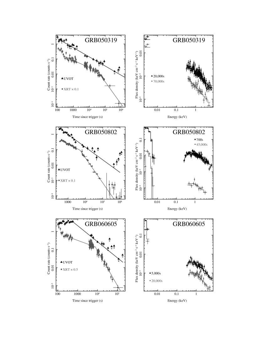
Figure 1: Lightcurves and SEDs of GRB050319, GRB050802, GRB060605. UVOT lightcurves are fitted by simple powerlaws, while XRT lightcurves and SEDs are fitted by broken powerlaws

The X-ray lightcurve of GRB050319 (Fig 1, top panel) shows the typical canonical behaviour, and can be adequately fitted by a double broken powerlaw model, which yields $\chi=113.3$ for 113 d.o.f.. The best fit parameters are decay indices of $\alpha_{X,1}=1.45^{+0.10}_{-0.11}$, $\alpha_{X,2}=0.48\pm 0.03$, $\alpha_{X,3}=1.41^{+0.08}_{-0.07}$ and break times among these segments of $t_{X,1}=300^{+60}_{-30}$ s and $t_{X,2}=29.9^{+2.6}_{-2.8}$ ks. The early, relatively steep decay is likely the tail of the prompt emission, a mechanism that does not involve the forward shock; we will therefore ignore this part of the emission hereafter. The initial flat decay phase, between $t_{X,1}$ and $t_{X,2}$, has a spectrum with a powerlaw index $\beta_{X,2}=1.00\pm 0.03$. After $t_{X,2}$, the X-ray spectrum shows marginal indication of softening, since the best fit index is $\beta_{X,3}=1.12\pm 0.07$.

The fit of the optical lightcurve (Fig.1, top panel) with a single powerlaw provides a marginally acceptable fit, yielding $\chi^{2}=54.6$ with 25 d.o.f. The best fit decay index is $\alpha_{O}=0.62\pm 0.02$. A fit with a broken powerlaw is slightly better, yielding $\chi^{2}=43.2$ for 23 d.o.f. The F-test indicates that the probability of chance improvement is very marginal, $6.5\%$. As for the broken powerlaw model, the values of the best fit parameters, other than the first slope, are not well constrained, if we leave all of them free to vary. We then fixed the value of the second slope, forcing it to differ from the first decay slope as much $\alpha_{X,2}$ differs from $\alpha_{X,3}$. We thus obtained $\alpha_{O,1}=0.58\pm{0.03}$, $\alpha_{O,2}=1.52$ for the two decay indices, and a break time $t_{O}=164.4^{+104.7}_{-79.5}$ ks. To find a strong upper limit on $t_{O}$, we varied its value while fitting the other parameters, until we obtained $\Delta\chi^{2}$ of 9. We found that we have $t_{O}>51.5$ ks at 3 sigma confidence level. Therefore, we note that a break in the optical band, if any, takes place much later than the break in the X-ray. Our result are consistent with those of Panaitescu et al. 2006, in which the authors do not find any steepening of the optical band emission up to $\sim 400$ks after the trigger. All these findings indicate that GRB050319 has got a genuine chromatic break in the X-ray band only at about 30ks after the trigger.

The SEDs of GRB050319 were built at 20ks and 70ks after the trigger (Fig. 1, top panel); results of the fit are shown in Table 3. For both SEDs, the fit with a cooling break in the spectrum yields a better $\chi^{2}$ than the fit with a single powerlaw, which is nevertheless still acceptable. In the following we will discuss both the cases of unbroken and broken powerlaws.

Let us first consider a scenario in which the X-ray and optical bands lie on the same spectral segment at 20ks, below the cooling frequency. This corresponds to the spectral fit with a single powerlaw of slope $\beta_{OX,E}=0.84\pm 0.05$. In this scenario, one should expect that the fluxes of both bands decay with the same slope. We find that the X-ray slope observed at early times, $\alpha_{X,2}=0.48\pm 0.03$, is consistent within $\sim 2.4\sigma$ with $\alpha_{O,1}=0.58\pm 0.03$. The average decay index of X-ray and optical is $\overline{\alpha}=0.53\pm 0.02$. Such a shallow optical decay requires that energy injection takes place. The value of the energy injection parameter $q$ is linked to the values of the spectral and decay indices ($\beta$ and $\alpha$) through the expression collected in Tab. 2 (Zhang et al. 2006, Panaitescu et al. 2006b). In the case at hand, we have $q=0.50\pm 0.06$ in the standard hypothesis of a constant density environment (ISM). The break in the X-ray lightcurve at 30 ks is generally interpreted as the cessation of energy injection. However, if this were the right scenario, the optical emission decay slope would simultaneously increase up to $\alpha=3\beta_{OX,E}/2=1.26\pm 0.08$, similar to the X-ray decay slope. This prediction is not consistent with our analysis. Alternatively, if the 30 ks break in the X-ray band were due to the transit of the cooling frequency below the X-ray band and not to the end of energy injection, the expected post-break decay index would be (Tab.2) $\alpha=0.95\pm 0.08$ whereas the observed value is $\alpha_{X,3}=1.41^{+0.08}_{-0.07}$. Another possibility would be that the cooling frequency is already between the optical and the X-ray bands at the time of the first SED. This corresponds to the broken powerlaw fits, where we find a low energy spectral slope $\beta_{OX,E}=0.49\pm 0.05$ at 20 ks and $\beta_{OX,L}=0.58^{+0.19}_{-0.12}$ at 70ks. The corresponding high energy spectral slopes are set to be higher by 0.5. If the cooling break is between the two bands, the only scenario that can explain why the X-ray flux decays slower than the optical, before the break at 30ks, is one in which the density profile of the circumburst medium is typical of a wind ejected by a massive star (with density decreasing as $r^{-\delta}$ where $r$ is the distance from the centre of the explosion and $\delta\sim 2$; see Chevalier & Li 2000). However, even this scenario cannot explain the decay slopes of X-ray flux and optical emissions after the 30ks break. In fact, the conventional interpretation of the canonical X-ray lightcurve is that after the 30 ks break the ejecta do not undergo any further increase of their kinetic energy. Without energy injection, in a wind environment, the decay slope above the cooling frequency would be less steep than that of the optical by $0.25$, which is obviously not in agreement with our observations. For example, the optical slope we would expect is $\alpha=\frac{3}{2}\beta+1/2$, where $\beta$ is the spectral slope in this band. Taking $\beta$ as the weighted average of the low energy spectral slopes, the optical decay should be $\alpha_{O}=1.25\pm 0.08$, and the X-ray decay should be $\alpha_{X}=\alpha_{O}-0.25=1.00\pm 0.08$, which is evidently in contrast with our findings.

In summary, this shows that the steep late X-ray decay is not explained if we assume that X-ray and optical are originated by the same component.
We can now demonstrate that the late X-ray break can be easily explained as a jet break, under the assumptions that the outflow responsible for the X-ray is different from that producing the optical emission, and the energy injection rate does not change till the end of the observations. Here and in the following, we will only consider the simple case of side-spreading jet and constant density medium with the addition of energy injection (Panaitescu et al. 2006b, but see § 4 for a discussion). In such a model, the energy is assumed to increase as a simple powerlaw, $E\propto t^{(1-q)}$, and the energy injection parameter $q$ does not change with time. To compute the value of $q$, we need the decay and spectral slopes, as in previous cases. In the X-ray, decay index is $\alpha_{X,2}=0.48\pm 0.03$, while for the spectral index we can take the weighted average of the energy index found by the X-ray data analysis throughout the whole lightcurve, $\overline{\beta}_{X}=1.02\pm 0.03$. With these values of parameters and in the case of the X-ray band above $\nu_{C}$, we derive (Tab. 2) $q=0.46\pm 0.06$. If there were not such energy injection, the decay slope after the jet break would become $\alpha=2\beta=2.04\pm 0.06$; but the addition of energy into the blastwave flattens the slope, leaving the flux decaying with $\alpha=1.31\pm 0.10$, a value which is within $1\sigma$ from the observed one, $\alpha_{X,3}=1.41^{+0.08}_{-0.07}$.

In order to compute the size of the beaming angle, $\theta$, of the narrow outflow, we use the expression (Frail et al. 2001):

$$\theta=0.093\left(\frac{t_{j,d}}{1+z}\right)^{3/8}{E_{k,52}}^{-1/8}\left(\frac{n}{0.1}\right)^{1/8}\,{\rm rad}\,,$$ (1)

where $t_{j,d}$ is the jet break time in days, $E_{k,52}$ is the isotropic kinetic energy of the outflow, and $n$ is the density of the environment in protons per cubic centimetre.

As we will discuss later on (see § 4), in order for our model to hold the kinetic energy in the outflow responsible for the X-ray emission should be of order $\sim 10\%$ of the whole energy of the ejecta (Scenario B, see par. 4). Furthermore, both the density $n$ of the environment and the efficiency $\eta$ of the conversion of kinetic energy into gamma rays should be moderately low. We assume $n=5\times 10^{-3}$ and $\eta\sim 0.01$. In order to derive an estimate of the energy produced by this burst, we look at the prompt emission fluence and spectrum. GRB050319 prompt emission between 20 and 150 keV was fitted by a single powerlaw spectrum, with photon index $\Gamma=2.1$ and had a fluence of $1.1\times 10^{-6}$ ergs cm^-1 (Cusumano et al. 2006). If we assume that the prompt emission spectrum of this GRB is described by the Band function, with spectral break below 20 keV and a typical low energy photon index 1, we find that this burst emitted $7\times 10^{52}$ ergs in the 1-10000 keV band, on the basis of isotropic emission at redshift z=3.24. Under the previous assumption on efficiency, density and fraction of total energy which goes into the narrow outflow, a jet break at 30 ks is compatible with a beaming angle of $\theta_{N}=0.015$ rad.

We note that, strictly speaking, in Eq 1, we should have taken into account that the energy of the ejecta is increasing during the afterglow. Nevertheless, considering the weak dependence of $\theta$ on $E_{k,52}$, the value of $\theta$ we found can be considered correct within a factor 2.

GRB	$\alpha_{O}$	$\alpha_{X,2}$	$\beta_{X,2}$	$t_{X,2}$ (ks)	$\alpha_{X,3}$	$\beta_{X,3}$
050319	$0.62\pm 0.02$	$0.48\pm 0.03$	$1.00\pm 0.03$	$29.93^{+}{2.55}_{-2.80}$	$1.41^{+0.08}_{-0.07}$	$1.12\pm 0.07$
050802	$0.82\pm 0.03$	$0.63\pm 0.03$	$0.89\pm 0.04$	$5.0\pm 0.3$	$1.59\pm 0.03$	$0.88\pm 0.04$
060605	$0.83\pm 0.04$	$0.41\pm 0.03$	$1.04\pm 0.07$	$7.73\pm 0.38$	$1.93^{+0.11}_{-0.10}$	$1.20\pm 0.09$
050401		$0.56\pm 0.02$	$0.99\pm 0.02$	$4.27\pm 0.52$	$1.44\pm 0.07$	$0.95\pm 0.07$
050607		$0.54^{+0.09}_{-0.10}$	$1.04\pm 0.14$	$16.2^{+6.4}_{-4.2}$	$1.33^{+0.16}_{-0.11}$	$1.17\pm 0.20$
050713A		$0.58\pm 0.03$	$1.27\pm 0.04$	$7.54^{+0.87}_{-0.80}$	$1.21\pm 0.03$	$1.02\pm 0.05$

Table 1: Results of the analysis of the bursts with chromatic breaks considered in this paper. From left to right: burst name, decay index in the optical, X-ray decay slope of the plateau phase, X-ray spectral slope in the plateau phase, X-ray lightcurve break time, X-ray late times decay index, X-ray late times spectral slope

		no injection		injection
	$\beta$	$\alpha$	$\alpha(\beta)$	$\alpha$	$\alpha(\beta)$
ISM and spehrical expansion
$\nu_{m}<\nu<\nu_{c}$	${{p-1\over 2}}$ (0.7)	${3(p-1)\over 4}$(1.05)	$\alpha={3\beta\over 2}$	${(2p-6)+(p+3)q\over 4}$ (0.38)	$\alpha=(q-1)+\frac{(2+q)\beta}{2}$
$\nu>\nu_{c}$	${{p\over 2}}$ (1.2)	${3p-2\over 4}$ (1.30)	$\alpha={3\beta-1\over 2}$	${(2p-4)+(p+2)q\over 4}$ (0.75)	$\alpha=\frac{q-2}{2}+\frac{(2+q)\beta}{2}$
ISM and jet expansion
$\nu_{m}<\nu<\nu_{c}$	${p-1\over 2}$ (0.7)	$p$ (2.4)	$\alpha=2\beta+1$	${(2p-3)+(p+3)q\over 3}$ (1.5)	$\alpha={(4\beta-1)+2(\beta+2)q\over 3}$
$\nu>\nu_{c}$	${{p\over 2}}$ (1.2)	$p$ (2.4)	$\alpha=2\beta$	${2(p-1)+(p+2)q\over 3}$ (1.67)	${2(q-1)\over 3}+{2(1+q)\beta\over 3}$
Wind and spherical expansion
$\nu_{m}<\nu<\nu_{c}$	${p-1\over 2}$ (0.7)	${3p-1\over 4}$ (1.55)	$\alpha={3\beta+1\over 2}$	${(2p-2)+(p+1)q\over 4}$ (1.13)	$\alpha=\frac{q}{2}+\frac{(2+q)\beta}{2}$
$\nu>\nu_{c}$	${p\over 2}$ (1.2)	${3p-2\over 4}$ (1.3)	$\alpha={3\beta-1\over 2}$	${(2p-4)+(p+2)q\over 4}$ (0.75)	$\alpha=\frac{q-2}{2}+\frac{(2+q)\beta}{2}$

Table 2: Table with the relations between the value of decay index $\alpha$ and the spectral slope $\beta$ in various afterglow models with the inclusion of the cases of energy injection. The case of $p<2$ is not included, and the self-absorption effect is not discussed. We do not consider the case of observing frequencies below $\nu_{m}$. The convention $F_{\nu}\propto t^{-\alpha}\nu^{-\beta}$ is adopted here. The temporal indices with energy injection are valid only for $q<1$, and they reduce to the standard case (without energy injection: Sari et al. 1998, Chevalier & Li 2000; with Energy injection: Zhang et al. 2006, Panaitescu et al 2006b) when $q=1$. For $q>1$ the expressions with energy injection are no longer valid, and the standard model applies. The numerical values quoted in parentheses are for $p=2.4$ and $q=0.5$.

	Fit at 20 ks			Fit at 70 ks
Parameters	Single powerlaw	Broken powerlaw		Single powerlaw	Broken powerlaw
$\beta_{1}$	$0.88^{+0.04}_{-0.04}$	$0.49\pm 0.05$		$0.84\pm 0.05$	$0.58^{+0.19}_{-0.12}$
$E_{B}$		$0.20^{+0.24}_{-0.14}$			$0.28^{+0.06}_{-0.05}$
$\beta_{2}$		$0.99\pm 0.05$			$1.08^{+0.19}_{-0.12}$
$E_{B-V}$	$13.1^{+1.9}_{-1.6}\times 10^{-2}$	$4.1^{+3.0}_{-2.7}\times 10^{-2}$		$8.80^{+0.45}_{-0.47}\times 10^{-2}$	$4.0^{+2.9}_{-1.7}\times 10^{-2}$
$N_{H}$	$<0.56$	$0.62\pm 0.20$		$<0.23$	$<0.87$
$\chi_{\nu}$	$129.5/108$	$110/107$		$34.6/24$	$22.2/23$

Table 3: Best fit values of the GRB050319 SED at 20 ks and 70 ks. $N_{H}$ is expressed in units of $10^{22}$ cm^-2, the break energy $E_{B}$ is given in keV, and the local extinction $E_{B-V}$ is in magnitudes. All upper limits are at 90% c.l..

	Fit at 20 ks			Fit at 70 ks
Parameters	Single powerlaw	Broken powerlaw		Single powerlaw	Broken powerlaw
$\beta_{1}$	$0.86\pm 0.02$	$0.89\pm 0.04$		$0.99\pm 0.02$
$E_{B}$		$4^{+5}_{-3}\times 10^{-3}$
$\beta_{2}$		$1.39\pm 0.04$
$E_{B-V}$	$18\pm 2\times 10^{-2}$	$18\pm 0.02\times 10^{-2}$		$0.18$
$N_{H}$	$0.26\pm 0.04$	$0.29\pm 0.04$		$0.26$
$\chi_{\nu}$	$120/104$	$119/103$		$27/15$

Table 4: Best fit values of the GRB0500802 SED at 0.4-1 ks and 35-55 ks. $N_{H}$ is expressed in units of $10^{22}$ cm^-2, the break energy $E_{B}$ is given in keV, and the local extinction $E_{B-V}$ is in magnitudes. In the case, the fit of the two SEDs was performed by assuming a Galactic extinction law (all results are taken from Oates et al. 2007).

3.2 GRB050802

In the case of GRB050802, we only briefly summarize the results obtained by Oates et al. (2007); the X-ray and optical lightcurves are shown in Fig.1 (middle panel). The X-ray lightcurve breaks from a decay slope of $\alpha_{X,2}=0.63\pm 0.03$ to a slope of $\alpha_{X,3}=1.59\pm 0.03$, $5.0\pm 0.3$ ks after the trigger. The optical lightcurve is well fitted by a single powerlaw decay with slope $\alpha_{O}=0.82\pm 0.03$; the $3\sigma$ lower limit on any possible break in the optical is t=$19$ks. Two SEDs were built at 500s and 40ks after the trigger (Fig. 1, middle panel). In the case of GRB050802, the best fit was provided by adopting the Gal model. Therefore, for this burst, the extinction was determined by applying this law. By applying the extinction determined in the early SED to the late time SED, it was determined that the late UV/optical emission lies above the extrapolated X-ray spectrum. This indicates that the optical emission is not produced by the same outflow that is responsible for the X-ray emission, regardless of where the synchrotron peak frequency and cooling frequency lie. Instead, the double component scenario described earlier was found to be consistent with the data if the X-ray band lies below the synchrotron cooling frequency $\nu_{C}$. In this case, with the values of parameters $\alpha_{X,2}=0.63\pm 0.03$ and $\beta_{X}=0.88\pm 0.04$ we can derive $q=0.51\pm 0.06$ If the break at 5 ks is interpreted as a jet break, the expected post-break slope would be (see again Panaitescu et al., 2006) $\alpha=2\beta+1=2.76\pm 0.08$ in case the decay proceeds without further energy injection, and $\alpha=1.83\pm 0.17$ in case there is no cessation of energy injection, which is consistent with the observed value of $\alpha_{X,3}$ within $2\sigma$. Results of the analysis are shown in Tables 1 and 4.

3.3 GRB050922c

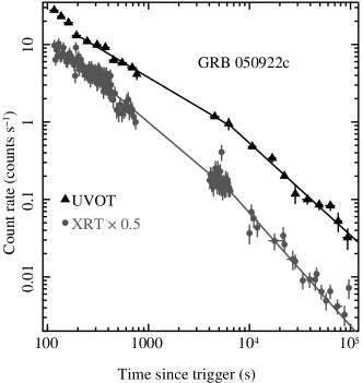
Figure 2: XRT and UVOT lightcurves of GRB050922c, the solid lines are the best-fitting broken powerlaws.

A first inspection of GRB050922c data clearly shows a break in the optical and XRT lightcurves (Fig. 2). In order to quantify its significance, we fit the lightcurves with a single and a broken powerlaw. The early optical emission shows some features superimposed on the powerlaw decay, such as an evident bump at $\sim 150$s after the trigger. Therefore, we excluded from the fit UVOT data taken during the first 200s after the trigger and, for consistency, we did this with the X-ray data as well. In the case of the X-ray lightcurve, we found that the fit with an unbroken powerlaw yields $\chi^{2}=219$ for 119 d.o.f., while a fit with a broken powerlaw provides an $\chi^{2}=141$ for 117 d.o.f.. The Ftest (Bevington et al. 1969) indicates that the probability of improvement by chance is less than $7\times 10^{-12}$. For a broken powerlaw, the best fit parameters are: initial decay slope $\alpha_{X,2}=1.10\pm 0.02$, break time $t_{X,b,2}=6.45^{+1.83}_{-0.76}$ ks, and late decay slope $\alpha_{X,3}=1.48^{+0.06}_{-0.04}$. For the optical lightcurve, a single powerlaw fit of the renormalised V, B and U band lightcurves gives $\chi^{2}=110.2$ for 18 d.o.f., whereas a broken powerlaw gives $\chi^{2}=24$ for 16 d.o.f.. In the latter case, the best fit parameters are $\alpha_{O,1}=0.77\pm 0.03$, $t_{O,b}=6.23^{+1.16}_{-0.99}$ ks, and $\alpha_{O,2}=1.20\pm 0.05$. As we can see, from our reanalysis and new reduction of the X-ray and optical data, the break times in the two bands turn out to be consistent with each other within 1$\sigma$, suggesting that the break in the X-ray lightcurve should not be considered as achromatic, in contrast to what was suggested by Panaitescu et al. (2006a).

3.4 GRB060605

The Swift GRB060505 also shows a canonical X-ray lightcurve, with an initial steep decay, a shallow plateau and finally a steep decay (Fig. 1, bottom panel). The decay slopes of the three segments and the two break times are $\alpha_{X,1}=2.68^{+0.92}_{-0.52}$, $t_{X,1}=164.5^{+29.9}_{-15.6}$s, $\alpha_{X,2}=0.41\pm 0.03$, $t_{X,2}=7.73\pm 0.38$ ks, $\alpha_{X,3}=1.93^{+0.11}_{-0.10}$. There is no evident strong X-ray spectral evolution, since the X-ray energy index in the plateau and in the steep decay are $\beta_{X,2}=1.04\pm 0.07$ and $\beta_{X,3}=1.20\pm 0.09$, consistent within $1\sigma$. In the optical, GRB060605 shows a wide peak at few hundreds seconds after the trigger, which is likely to be the beginning of the forward shock emission (Oates et al. in prep.). In fitting the optical lightcurve (Fig. 1, bottom panel), we considered all the datapoints taken after 500s from the trigger. The single powerlaw model provides a marginally acceptable fit, with $\chi^{2}=28$ for 13 d.o.f.. We then tried a broken powerlaw model, which gives a much better fit with $\chi^{2}=10.6$ for 10 d.o.f.. The value of the late decay slope is $\alpha_{O,2}=3.3^{+\infty}_{-1.0}$, but it is not well constrained; we can infer that it has a lower limit of $1.4$ at 95% C.L.. The best fit values of the other parameters are $\alpha_{O,1}=0.85\pm 0.04$ and $t_{O}=23.5^{+5.9}_{-4.0}$ ks. The 3$\sigma$ lower limit on the break time in the optical, calculated as in the case of GRB050319, is $t_{O}=12.3$ ks. Ferrero et al. (2008) present a dataset in which the optical afterglow is well detected till $\sim 1$ day after the trigger, and their data show an evident break occurring 23.3 ks after the trigger, with a late decay slope $\alpha_{O,2}=2.56\pm 0.16$. We note that our best fit values are consistent with those of Ferrero et al. (2008). Thus, we can conclude that a break is present in the optical, but it is inconsistent with $t_{X,2}$. Ferrero et al. (2008) suggest that the different break times might be caused by some flaring activity in the X-ray band that occurred around 6ks after the trigger. These flares would have led to the conjecture of an X-ray afterglow decaying shortly thereafter (see their paper for more details). We will rather investigate the scenario in which GRB060605 has a genuine chromatic break. For this GRB, we built up the SEDs at 5ks and 20ks; the values of the best fit parameters are reported in Table 5. As we can see, we cannot distinguish between the single powerlaw and the broken powerlaw spectral fit on statistical basis, since both models provide a similar reduced $\chi^{2}$. However, an unbroken powerlaw model is ruled out by the fact that X-ray and optical decay slopes are inconsistent at $7\sigma$ level at 5 ks and $10\sigma$ level at 20 ks. We are thus left with a scenario in which the spectrum is a broken powerlaw at 5 ks and 20 ks. Furthermore, we have to assume a wind circumburst environment for the same reasons quoted for GRB050319. We reiterate that, in this environment, the cooling frequency is supposed to increase.

If we fit the two SEDs with a broken powerlaw and restrict the break energy between 0.005 and 1 keV, the low energy spectral indeces are $\beta_{OX,E}=0.54\pm 0.07$, $\beta_{OX,L}=0.71\pm 0.09$, at 5 and 20 ks respectively. The break energy at 5ks is $0.008$ keV, with a 1 $\sigma$ positive error of $0.032$. This break energy value is near the minimum allowed value of $0.005$ keV; we were not able to find an 1$\sigma$ negative error.

We note that the low energy spectral indices are consistent within $2\sigma$. We assume an average low index $\overline{\beta}_{OX}=0.60\pm 0.06$ and a high energy index $\overline{\beta}_{OX}+0.5=1.10\pm 0.06$ respectively. The first index has got to be that of the Optical band. In the usual interpretation of the canonical X-ray lightcurve, the break at 7.3ks corresponds to the end of energy injection into the ejecta. If this is the right scenario, in a wind density profile, the optical emission decay index should be higher than that of the X-ray emission by 0.25. For example, we should observe an optical decay slope $\alpha_{O}=\frac{3}{2}\overline{\beta}_{OX}+1/2=1.40\pm 0.09$ after the end of the injection; the X-ray flux decay index ought to be $\alpha_{X}=\alpha_{O}-0.25=1.15$. These predictions are clearly inconsistent with the observed behaviour. The X-ray flux would decay faster than 1.15 if the cooling frequency moved above the X-ray band, but in such a case the X-ray decay slope would be consistent with that of the optical, which is inconsistent with observations, as stated above.

We try now to apply our model to interpret the behaviour of the X-ray emission for this burst. Again, the idea is that the plateau, extending till $7.3$ ks after the trigger, is due to forward shock emission of ejecta expanding like they were spherical, with the contribution of energy injection. For this burst, we suppose that the X-ray band remains below the cooling frequency. In fact, by using $\alpha_{X,2}$ and the weighted average energy index $\overline{\beta}_{X}=1.10\pm 0.06$, from Tab. 2 we derive $q=0.20\pm 0.06$. Assuming that the end of the plateau phase is due to a jet break with side expansion, the predicted decay slope post break would be $\alpha=3.20\pm 0.12$ or $\alpha=1.48\pm 0.20$ in case of cessation or continuation of the energy injection, respectively (see Tab.2). Again, the second value is consistent with the observed result at $2\sigma$ level ( $\alpha_{X,3}=1.93^{+0.11}_{-0.10}$). In order to compute the opening angle $\theta_{N}$ of the outflow responsible for the X-ray emission, we can follow the same procedure as GRB050319 after estimating the total emitted energy. According to Sato et al.(2006), the fluence in the 15-150 keV band of GRB060605 is $4.6\times 10^{-7}$ erg cm^-2, while the spectrum is best fitted by a simple powerlaw with photon index $\Gamma_{1}\sim 1.34$. Since this value suggests a high energy spectrum below the break energy (Band et al. 1993), we can assume that the break energy is occurring just above the BAT bandpass. Assuming that the high energy photon index is $\Gamma_{2}=2.3$ (the average value for this parameter following Band et al. 1993) and redshift $z=3.8$, we find that the isotropic energy emitted between 1 and 10000 keV is $E\sim 3.5\times 10^{52}$ ergs. The next step is to estimate the kinetic energy of the ejecta and which fraction of it goes into the narrow outflow. Now, in the case of GRB060605, a possible jet break occurs in the optical not much later than the jet break in the X-ray, Eq. 1 indicates that the opening angle $\theta_{W}$ of the outflow responsible for the optical emission and $\theta_{N}$ could be close. Now, in our modelling (see section 4 for details), it is intrinsically assumed that we have emissions from spherical portions of two outflows, and the emitting surface of the narrow outflow, responsible for the X-ray emission, is much less than the surface of the wide outflow, which is producing the optical emission. The approximation can hold if the beaming angles of the two outflows are different enough. A way we can reconcile our interpretation with the features of GRB060605 is by assuming that the energy in the narrow component $E_{N}$ is much higher than the energy $E_{W}$ carried by the wide outflow. In our theoretical discussion, we have found that solutions with $E_{N}\simeq 30E_{W}$ are possible (Scenario A”, see section 4). This solutions applies in cases of density $n\simeq 1$, and efficiency of conversion of kinetic energy of the ejecta into $\gamma$-ray emission $\eta=0.2$. We thus derive that the kinetic energy of the ejecta is $\sim 1.8\times 10^{53}$ ergs. Now, if we apply this ratio of energies and this density to GRB060605, then we derive, by using Eq. 1, that the narrow outflow should have an opening angle $\theta_{N}=0.019$ rad. The outflow responsible for the optical emission should have $\theta_{W}=0.05$.

	Fit at 5 ks			Fit at 20 ks
Parameters	Single Pow.	Broken Pow.		Single Pow.	Broken Pow.
$\beta_{1}$	$1.01^{+0.07}_{-0.06}$	$0.54\pm 0.07$		$1.16\pm 0.09$	$0.71\pm 0.09$
$E_{B}$		$0.008^{+0.032}$			$0.375^{+0.215}_{-0.350}$
$\beta_{2}$		$1.54\pm 0.07$			$1.21\pm 0.09$
$E_{B-V}$	$7.64^{+2.16}_{-0.64}\times 10^{-2}$	$0.008^{+0.032}$		$12.5^{+0.5}_{-0.6}\times 10^{-2}$	$<0.122$
$N_{H}$	$<0.96$	$0.49^{+0.24}_{-0.24}$		$1.28^{+0.46}_{-0.43}$	$1.48^{+0.71}_{-0.64}$
$\chi_{\nu}$	42.0/42	$41.4/41$		$28.4/27$	$26.4/26$

Table 5: Best fit values of the GRB060605 SED at 5 ks and 20 ks. $N_{H}$ is expressed in units of $10^{22}$ cm^-2, the break energy $E_{B}$ is given in keV, and the local reddening $E_{B-V}$ is in magnitudes. Upper limits on column density and reddening are at 90% c.l..

GRB	Observed $\alpha_{X,3}$	Predicted $\alpha_{X,3}$	$\theta_{N}$
050319	$1.41^{+0.08}_{-0.07}$	$1.31\pm 0.10$	0.015
050802	$1.59\pm 0.03$	$1.83\pm 0.17$	0.017
060605	$1.93^{+0.11}_{-0.10}$	$1.48\pm 0.20$	0.019
050401	$1.44\pm 0.07$	$1.74\pm 0.09$	0.006
050607	$1.33^{+0.16}_{-0.11}$	$1.57\pm 0.41$	0.023
050713A	$1.21\pm 0.03$	$1.44\pm 0.11$	0.008

Table 6: GRBs with chromatic breaks considered in this work. The table shows the late decay slope observed in the X-ray, the slope predicted by our model, and the inferred values of the beaming angle for the narrow outflow. In the case of GRB050802, values are taken by Oates et al. (2007).

3.5 GRBs with X-ray data analysis only

All the bursts for which we built the optical and X-ray SEDs have their redshift known by spectroscopy, while the following other objects in our sample do not have known redshifts (except 050401). However, since they are studied in the X-ray band only, the lack of a redshift basically does not affect our results and conclusions.

GRB050401 - A break is evident in the X-ray lightcurve of this GRB: the decay slope changes from $\alpha_{X,2}=0.56\pm 0.02$ to $\alpha_{X,3}=1.44\pm 0.07$ at $t_{X,2}=4.27\pm 0.52$ ks. There is not strong spectral evolution throughout the whole observation, since the spectral index is always consistent with $\beta_{X}=0.99\pm 0.02$. Again, if the X-ray band is below $\nu_{C}$, then the energy injection parameter would be $q=0.39\pm 0.03$. If the outflow responsible for the X-ray emission underwent a jet break without energy injection, the predicted slope of the flux decay would be $\alpha=2.98\pm 0.04$, which is inconsistent with the value we observe. However, in the presence of energy injection the predicted value is $\alpha=1.74\pm 0.09$, which is consistent with the observed X-ray decay slope at $\sim 2.3\sigma$ level. In order to compute the beaming angle of the outflow responsible for the X-ray emission, we need to make some assumptions. We will assume that the Energy of narrow outflow responsible for the X-ray emission is $10\%$ that of the a wider outflow that produces the optical emission (Scenario B), and an efficiency $\eta=0.01$ and a density $n=5\times 10^{-3}$. We have $E_{\gamma}=3.5\times 10^{53}$ ergs (Golenetskii et al. 2005). With these assumptions for density, efficiency and ratios of kinetic energies the jet beaming angle of the narrow component turns out to be $\theta_{N}=0.006$ rad (Eq. 1).

GRB050607 - This burst exhibits an evident break in the X-ray lightcurve, since its decay slopes change from $\alpha_{X,2}=0.54^{+0.09}_{-0.10}$ to $\alpha_{X,3}=1.33^{+0.16}_{-0.11}$ at $16.2^{+6.4}_{-4.2}$ ks. The X-ray spectrum does not show evidence of evolution at the break time and has an average energy index of $\beta_{X}=1.07\pm 0.11$. Assuming that the X-ray band is above the cooling frequency, the values of $\beta_{X}$ and $\alpha_{X,2}$ imply $q=0.59\pm 0.23$ (Tab. 2). Without late time energy injection, the subsequent jet decay slope would be $\alpha=2.14\pm 0.22$, while with energy injection the predicted value is $\alpha=1.57\pm 0.41$. The latter is consistent with the observed value of $\alpha_{X,3}$, within $\sim 1\sigma$. In order to derive the beaming angle of the narrow outflow, we need an estimate of the burst energetics. Since the redshift of this burst is presently unknown, we adopted $z=2.5$ (i.e. about the average Swift GRB redshift, Jakobsson et al. 2006) and a prompt emission spectral index estimated by the Band function, with a high energy photon index of $\sim$ 2.1 in the energy band from 15 keV to 10000 keV and of $\sim$1 below 15 keV (Pagani et al. 2006 report $1.83\pm 0.14$ in the range 15-150 keV). Under this hypothesis, the energy emitted by the burst would be $\sim 2.4\times 10^{52}$ ergs. We can assume that 90% of the kinetic energy of the outflows is carried by the broad one, and we can take $\nu_{c}$ below the X-ray band (scenario B, section 4); other assumptions are $n=5\times 10^{-3}$, $\eta=0.01$. With these hypothesis in place, we obtain a beaming angle of $\theta_{N}=0.023$ rad.

GRB050713A - the X-ray lightcurve of this burst shows a break at $t_{X,2}=7.54^{+0.87}_{-0.80}$ ks, after which the decay slope increases from $\alpha_{X,2}=0.58\pm 0.03$ to $\alpha_{X,3}=1.21\pm 0.03$. The spectral index, throughout the whole observation, is $\beta_{X}=1.17\pm 0.03$. The energy injection parameter, again for the case of X-ray band above $\nu_{C}$, is $q=0.38\pm 0.06$. The expected slope at late times would be $\alpha=2.34\pm 0.06$ or $\alpha=1.44\pm 0.11$ in case of cessation or continuation of the energy injection process, respectively. The latter is consistent with the observed decay slope in the X-ray band within 2$\sigma$. To calculate the beaming angle of the narrow outflow, we made again an assumption on the (currently unknown) burst redshift. By using $z=2.5$, and taking the values of fluence and spectral parameters published in Morris et al. (2007), we infer an isotropic $\gamma$-ray energy of $E_{\gamma}\sim 2.5\times 10^{53}$ ergs. With the same assumptions made for GRB050607, we obtain $\theta_{N}=0.008$ rad.

4 Discussion

Results reported in the previous section show that a single outflow model cannot explain the behaviour of the GRBs with chromatic breaks we have considered. Instead, we found that if the X-ray flux is attributed to ejecta which are decoupled from those responsible for the optical, the observed behaviours of these GRBs can be explained. In the theoretical modelling of GRBs, a double component outflow has already been put forward, even before the launch of Swift (e.g. Berger et al. 2003, Peng et al. 2005). It has been invoked to explain the complex temporal behaviour of X-ray and optical emissions of the exceptional GRB080319B (Racusin et al. 2008). In this section, we would like to explore the viability of the two-component jet model with the important addition of a continuous energy injection, from a theoretical point of view.

The basic picture is based on ejecta with two different degrees of collimation. The narrow outflow generates the X-ray emission, while the wide one the optical. Both emissions are due to the usual forward shock, which has a synchrotron spectrum consisting of powerlaws connected at particular frequencies (Sari, Piran & Narayan 1998), i.e. the synchrotron frequency $\nu_{m}$ and the cooling frequency $\nu_{c}$. In this paper, we use the expressions of $\nu_{m}$, $\nu_{c}$ and of the peak flux $F_{max}$ as determined in Zhang et al. (2007) for a constant density medium:

$$F_{max} = 1600(1+z)D_{28}\epsilon_{B,-2}^{1/2}E_{K,52}n^{1/2}\,{\rm\mu Jy}$$

$$\nu_{m} = 3.3\times 10^{12}\left(\frac{p-2}{p-1}\right)^{2}\left(1+z\right)^{1/2}\epsilon_{B,-2}^{1/2}\epsilon_{e,-1}^{2}$$

$$\times E_{K,52}^{1/2}t_{d}^{-3/2}\,{\rm Hz}$$

$$\nu_{c} = 6.3\times 10^{15}(1+z)^{-1/2}\epsilon_{B,-2}^{-3/2}E_{K,52}^{-1/2}n^{-1}t_{d}^{-1/2}\,{\rm Hz}\,,$$

where $z$ is the redshift, $D_{28}$ is the luminosity distance in units of $10^{28}$ cm, $\epsilon_{B,-2}$ and $\epsilon_{e,-1}$ are the ratios between the magnetic/electron and kinetic energy of the ejecta (in units of $10^{-2}$ and $10^{-1}$ respectively), $E_{52}$ is the isotropic kinetic energy as measured in the observer rest frame and normalized to $10^{52}$ ergs, $n$ is the particle density in cm^-3, $p$ is the index of the the powerlaw energy distribution of radiating electrons, and $t_{d}$ is the observer time in days.

By taking $z=2.5$ (as for an average Swift GRB, see previous sections) and a cosmology with $H_{0}=71,\Omega=0.3,\Lambda=0.7$, gives $D_{28}=6.2$. We adopt a typical value of $p=2.4$, which gives an energy index between $\nu_{m}$ and $\nu_{c}$ of $\beta=(p-1)/2=0.7$. Below $\nu_{m}$ we assume a standard synchrotron spectrum rising with $\beta=-1/3$. In order to take into account the energy injection, we assume that the luminosity of the GRB central engine scales as $L\propto t^{-q}$, with a typical value of $q=0.5$ (Zhang et al. 2006). This corresponds to an increase of kinetic energy of the ejecta of the kind $E\propto t^{(1-q)}=t^{0.5}$. All these assumptions allow us to recalculate the coefficient in the formulae of  4 and change the time dependencies, taking into account the increase in energy. We obtain

$$F_{max} = 2.55\times 10^{3}\epsilon_{B,-2}^{1/2}E_{52,0}n^{1/2}t_{d}^{1/2}\,{\rm\mu Jy}$$

$$\nu_{m} = 2.1\times 10^{12}\epsilon_{B,-2}^{1/2}\epsilon_{e,-1}^{2}E_{52,0}^{1/2}t_{d}^{-5/4}\,{\rm Hz}$$

$$\nu_{c} = 4.4\times 10^{14}\epsilon_{B,-2}^{-3/2}E_{52,0}^{-1/2}n^{-1}t_{d}^{-3/4}\,{\rm Hz}\,$$ (3)

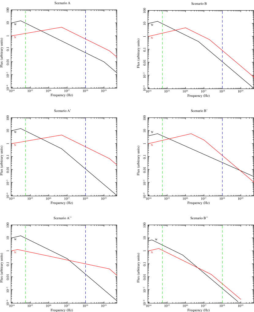
Figure 3: The 6 configurations of the wide (W) and narrow (N) components explored in the text. Vertical lines indicate the optical and X-ray band respectively.

where $E_{52,0}$ is the isotropic kinetic energy at 300s after the trigger. We chose this time because it is typically from 300s that the slow decline phase is observed in both the X-ray and optical afterglows. Furthermore, we require our scenario to work up to 0.1 days after trigger, since it is typically around $\sim 0.1$ days that the plateau phase ends. To distinguish between the narrow and wide component, we use the pedices “n” and “w” respectively, while “O” and “X” indicate the optical and X-ray band. For the optical and X-ray frequencies, we used the values $\nu_{O}=5.5\times 10^{14}$ Hz and $\nu_{X}=10^{18}$ Hz, respectively. Therefore, for instance, $f_{O,w}$ is the optical flux due to the wide component.
In the following treatment, we shall be discussing six possible scenarios. In order for our model to work, the narrow/wide component should not contribute significantly to the optical/X-ray flux. We translate this “condition of non-interference” by requiring that the optical flux of the narrow component is at maximum one half of that of the wide one, and a similar condition for the X-ray band. The six different scenarios we are considering reflect six different possible hierarchies between the various frequencies. Scenarios A and B deal with the case in which both $\nu_{c,n}$ and $\nu_{c,w}$ lie above or below the X-ray band, respectively. The next two cases, A’ and B’, are a variant of the previous ones, in which $\nu_{c,w}$ and $\nu_{c,n}$ do not lie on the same side with respect to the X-ray frequency. Cases A” and B” show the same arrangements of frequencies as A’ and B’, but the synchrotron peak frequency of the narrow component is below the optical since the beginning of observations. Our data do not allow to distinguish between the cases A, A’, and A” (or B, B’ and B”). We require $\nu_{m,w}<\nu_{O}$ and $\nu_{m,n}<\nu_{X}$, consistently with the absence of an increase in the optical and X-ray flux at early times in the datasets we have analyzed. All scenarios are summarized in Fig. 3. In § 4.7, we discuss the extension of validity of the conditions we pose after 0.1 d.

4.1 Scenario A

The conditions to apply in scenario A are:

$$f_{O,w}>2f_{n,O}\qquad{\rm at\,0.1\,d\,after\,the\,trigger.}$$ (4)

$$f_{X,w}<\frac{1}{2}f_{n,w}$$ (5)

$$\nu_{m,w}<\nu_{O}\qquad{\rm at\,300\,s\,after\,the\,trigger.}$$ (6)

$$\nu_{m,n}>\nu_{O}\qquad{\rm at\,0.1\,d\,after\,the\,trigger.}$$ (7)

$$\nu_{X}<\nu_{c,w}\qquad{\rm at\,0.1\,d\,after\,the\,trigger.}$$ (8)

$$\nu_{X}<\nu_{c,n}\qquad{\rm at\,0.1\,d\,after\,the\,trigger.}$$ (9)

$$\nu_{m,n}<\nu_{X}\qquad{\rm at\,300\,s\,after\,the\,trigger.}$$ (10)

It is easy to verify that, if the above conditions are satisfied at the time indicated, they are also valid for the whole interval in which we are interested, i.e. between 300s and 0.1 days after the trigger. Since the second condition describes the evolution of the flux below the cooling frequencies for both components, time dependencies cancel out. The first condition (Eq. 4) can be written as

$$\epsilon_{B,-2,w}^{1/2}E_{52,0,w}\left(\frac{5.5\times 10^{14}}{2.1\times 10^{12}\epsilon_{B,-2,w}^{1/2}\epsilon_{e,-1,w}^{2}E_{52,0,w}^{1/2}0.1^{-5/4}}\right)^{-0.7}$$ (11)

$$>2\epsilon_{B,-2,n}^{1/2}E_{52,0,n}\left(\frac{5.5\times 10^{14}}{2.1\times 10^{12}\epsilon_{B,-2,n}^{1/2}\epsilon_{e,-1,n}^{2}E_{52,0,n}^{1/2}0.1^{-5/4}}\right)^{1/3}$$

which, after some iterations, can be rearranged into

$$\epsilon_{B,-2,w}^{0.85}E_{52,0,w}^{1.35}\epsilon_{e,-1,w}^{1.4}>29.5\epsilon_{B,-2,n}^{1/3}E_{52,0,n}^{5/6}\epsilon_{e,-1,n}^{-2/3}\,.$$ (12)

Similarly, the second condition (Eq. 5) can be expressed as

$$\epsilon_{B,-2,w}^{1/2}E_{52,0,w}\left(\frac{10^{18}}{2.1\times 10^{12}\epsilon_{B,-2,w}^{1/2}\epsilon_{e,-1,w}^{2}E_{52,0,w}^{1/2}}\right)^{-0.7}$$ (13)

$$<\frac{1}{2}\epsilon_{B,-2,n}^{1/2}E_{52,0,n}\left(\frac{10^{18}}{2.1\times 10^{12}\epsilon_{B,-2,n}^{1/2}\epsilon_{e,-1,n}^{2}E_{52,0,n}^{1/2}}\right)^{-0.7}$$

which simplifies to

$$\epsilon_{B,-2,w}^{0.85}E_{52,0,w}^{1.35}\epsilon_{e,-1,w}^{1.4}<\frac{1}{2}\epsilon_{B,-2,n}^{0.85}E_{0,52,n}^{1.35}\epsilon_{e,-1,n}^{1.4}\,.$$ (14)

From these two inequalities we have

$$E_{52,0,n}>2.73\times 10^{3}\epsilon_{B,-2,n}^{-1}\epsilon_{e,-1,n}^{-4}\,.$$ (15)

We can now obtain a constraint on $E_{52,0,n}$ from Eq. 9

$$E_{52,0,n}<6.1\times 10^{-6}\epsilon_{B,-2,n}^{-3}n^{-2}\,,$$ (16)

which, substituted in Eq. 15, gives

$$\epsilon_{B,-2,n}<4.8\times 10^{-5}\epsilon_{e,-1,n}^{2}n^{-1}\,.$$ (17)

By substituting Eq. 17 into Eq. 15 and after some manipulating, we have

$$E_{52,0,n}>5.4\times 10^{7}\epsilon_{e,-1,n}^{-6}n\,.$$ (18)

From Eq. 18, we can infer that the value of $\epsilon_{e,-1,n}$ must be very high, in order to avoid an unreasonable value for the energy of the narrow outflow. By assuming $\epsilon_{e,-1,n}=3.3$, i.e. the maximum value (which is given at equipartition), we obtain $E_{52,0,n}>4\times 10^{4}n$. With this value of $\epsilon_{e,-1,n}$, a constraint on $\epsilon_{B}$ can now be obtained from Eq 17; by assuming $n=0.01$ it gives $\epsilon_{B,-2,n}<5\times 10^{-2}$, which is a very low value.

We try now to derive some constraints on the physical parameters of the wide component. By solving Eq. 12 for the parameter $E_{52,0,n}$ and substituting it into Eq. 14, we derive

$$E_{52,0,w}^{-0.79}\epsilon_{B,-2,w}^{-0.5}\epsilon_{e,-1,w}^{-0.8}<2.3\times 10^{-3}\epsilon_{B,-2,n}\epsilon_{e,-1,n}^{2.35}\,.$$ (19)

which can be combined with Eq. 8

$$E_{52,0,w}^{-1/2}\epsilon_{B,-2,w}^{-3/2}n^{-1}>404.4$$ (20)

to obtain

$$E_{52,0,w}>4\times 10^{6}n^{0.54}\epsilon_{e,-1,w}^{-1.29}\epsilon_{B,-2,n}^{-0.47}\epsilon_{e,-1,n}^{-3.8}\,.$$ (21)

Under the previous assumption of $\epsilon_{e,-1,n}=3.3$ and taking $\epsilon_{B,-2,n}=10^{-2}$, we derive $E_{52,0,w}>3.5\times 10^{4}\epsilon_{e,-2,w}^{-1.29}$. Again, the fraction of the energy given to the electrons must be close to equipartition, in order to avoid very high values of the energy of the wide component. If $\epsilon_{e,-2,w}\sim 3.3$, we obtain $E_{52,0,w}>8\times 10^{3}$. It is physically implausible to have a value of $E_{52,0,w}$ much higher than this lower limit. Apart from these caveats, we can now show that the set of inequalities assumed within scenario A cannot be simultaneously verified. In fact, Eq. 6 reads

$$\epsilon_{B,-2,w}^{1/2}\epsilon_{e,-1,w}^{2}E_{52,0,w}^{1/2}<0.221\,.$$ (22)

With the values we just obtained for $\epsilon_{e,-1,w}^{2}$ and $E_{52,0,w}$, Eq. 22 requires an extremely small value of the magnetic energy, $\epsilon_{B,-2,w}<10^{-9}$. On the other hand, by substituting the lower limits on $E_{52,0,n}$, $E_{52,0,w}$ and $\epsilon_{e,-1,n}=\epsilon_{e,-1,w}^{2}=3.3$ into Eq. 12 and  14, we can derive the following inequalities

$$8.8\times 10^{3}\epsilon_{B,-2,n}^{0.85}>10\times 10^{6}\epsilon_{B,-2,w}^{0.85}>2\times 10^{3}\epsilon_{B,-2,n}^{1/3}\,,$$ (23)

and, in turn, a lower limit on $\epsilon_{B,-2,n}>7.7\times 10^{-3}$. By substituting this value in the right member of Eq. 23 gives $\epsilon_{B,-2,w}>3.3\times 10^{-3}$, which is in contradiction with what was derived from Eq. 22.

4.2 Scenario A’

We now consider a variant of the previous scenario, in which the cooling frequency of the wide component lays below the X-ray frequency but above the optical band. As already mentioned, our model cannot distinguish between this scenario and that described in the previous subsection. The set of conditions expressed in Eqs. 4 - 10 are modified as follows:

$$f_{O,w}>2f_{O,n}\qquad{\rm at\,0.1\,d\,after\,the\,trigger.}$$ (24)

$$f_{X,w}<\frac{1}{2}f_{X,n}\qquad{\rm at\,300\,s\,after\,the\,trigger.}$$ (25)

$$\nu_{m,w}<\nu_{O}\qquad{\rm at\,300\,s\,after\,the\,trigger.}$$ (26)

$$\nu_{O}<\nu_{c,w}\qquad{\rm at\,0.1\,d\,after\,the\,trigger.}$$ (27)

$$\nu_{x}>\nu_{c,w}\qquad{\rm at\,300\,s\,after\,the\,trigger}$$ (28)

$$\nu_{x}>\nu_{m,n}\qquad{\rm at\,300\,s\,after\,the\,trigger}$$ (29)

$$\nu_{m,n}>\nu_{O}\qquad{\rm at\,0.1\,d\,after\,the\,trigger}$$ (30)

$$\nu_{x}<\nu_{c,n}\qquad{\rm at\,0.1\,d\,after\,the\,trigger\,.}$$ (31)

Notice that Eq. 30 must now hold at 0.1 days after the trigger, while Eq. 25 must be satisfied at 300s. These conditions are translated into the following inequalities:

$$\epsilon_{B,-2,w}^{0.85}E_{52,0,w}^{1.35}\epsilon_{e,-1,w}^{1.4}>29.5\epsilon_{B,-2,n}^{1/3}E_{52,0,n}^{5/6}\epsilon_{e,-1,n}^{-2/3}\,,$$ (32)

$$\epsilon_{B,-2,w}^{0.1}\epsilon_{e,-1,w}^{1.4}E_{52,0,w}^{1.1}<2.85\epsilon_{B,-2,n}^{0.85}\epsilon_{e,-1,n}^{1.4}E_{52,0,n}^{1.35}n^{1/2}$$ (33)

$$\epsilon_{B,-2,w}^{1/2}\epsilon_{e,-1,w}^{2}E_{52,0,w}^{1/2}<0.22$$ (34)

$$\epsilon_{B,-2,w}^{-3/2}E_{52,0,w}^{-1/2}n^{-1}>0.22$$ (35)

$$\epsilon_{B,-2,w}^{-3/2}E_{52,0,w}^{-1/2}n^{-1}<32.5$$ (36)

$$\epsilon_{B,-2,n}^{1/2}\epsilon_{e,-1,n}^{2}E_{52,0,n}^{1/2}<4\times 10^{2}$$ (37)

$$\epsilon_{B,-2,n}^{1/2}\epsilon_{e,-1,n}^{2}E_{52,0,n}^{1/2}>14.7$$ (38)

$$\epsilon_{B,-2,n}^{-3/2}E_{52,0,n}^{-1/2}n^{-1}>4\times 10^{2}\,.$$ (39)

By combining Eq. 34 with Eq. 36 we obtain

$$E_{52,0,w}<0.35\epsilon_{e,-1,w}^{-6}n\,.$$ (40)

In order not to restrict ourselves to solutions with very low $E_{52,0,w}$, we will assume a quite small value of $\epsilon_{e,-1,w}$

Rearranging Eq. 36, we derive a constraint on $\epsilon_{B,-2,w}$:

$$\epsilon_{B,-2,w}>0.10E_{52,0,w}^{-1/3}n^{-2/3}\,,$$ (41)

while solving Eq. 38 for $\epsilon_{B,-2,n}$ and substituting it into Eq. 39, we obtain

$$E_{52,0,n}>1.28\times 10^{6}\epsilon_{e,-1,n}^{-6}n\,.$$ (42)

From this last equation we infer that $\epsilon_{e,-1,n}$ cannot be very far from the maximum value of 3.3, achieved at equipartition, to avoid extremely high values of energy of the narrow outflow. If $\epsilon_{e,-1,n}=3.3$, then $E_{52,0,n}>10^{3}n$.

Finally, from Eq. 39 we obtain a constraint on $\epsilon_{B,-2,n}$

$$\epsilon_{B,-2,n}<0.019E_{52,0,n}^{-1/3}n^{-2/3}\,.$$ (43)

Now we will show that the previous set of inequalities can be solved simultaneously by assuming not unreasonable values of the physical parameters, provided that we limit ourselves to a scenario in which the circumburst density is relatively small, $n\sim 10^{-3}$, which makes the set of conditions easier to meet. Let us first assume that $\epsilon_{e,-1,n}=3.3$ and that the energy of the narrow component is, $E_{52,0,n}=5$. For the chosen values of these two parameters, Eq. 38 requires $\epsilon_{B,-2,n}>0.6$. Taking $\epsilon_{B,-2,n}=1$, from Eq. 34 and Eq. 32 we can derive a lower limit on the values of $E_{52,0,w}$. In fact, Eq. 32 becomes

$$\epsilon_{B,-2,w}^{0.85}\epsilon_{e,-1,w}^{1.4}E_{52,0,w}^{1.35}>50\,,$$ (44)

which, combined with Eq. 34, gives

$$\epsilon_{B,-2,w}^{0.5}E_{52,0,w}>150\,.$$ (45)

Now, the highest value possible of $\epsilon_{B,-2,w}$ is reached at the equipartition, $\epsilon_{B,-2,w}=33$; in such a case, $E_{52,0,w}>25$. By assuming a more reasonable value of $\epsilon_{B,-2,w}=10$ (Panaitescu & Kumar 2001b, Yost et al. 2003) give instead $E_{52,0,w}>50$.

By rearranging Eq. 32 and 34 we derive

$$\epsilon_{e,-1,w}^{-4}\epsilon_{B,-2,w}^{-0.5}>3\times 10^{3}$$ (46)

which, with the value of $\epsilon_{B,-2,w}$ chosen above, implies $\epsilon_{e,-1,w}<0.1$.

Let us assume the following series of parameters: $n=3\times 10^{-3}$, $\epsilon_{e,-1,n}=3.3$, $\epsilon_{B,-2,w}=10$, $\epsilon_{e,-1,w}=0.04$ and $E_{52,0,w}=600$. As we will explain in the following, larger values of $E_{52,0,w}$ are implausible, since they translate into unphysically high values of kinetic energy of the wide component at late times. Moreover, since our model requires a substantial difference in the beaming angles of the wide and narrow components, then the difference in the respective kinetic energies must not be too large. We then assume $E_{52,0,n}\approx 0.20E_{52,0,w}=120$, and $\epsilon_{B,-2,n}=0.1$ (the latter to satisfy Eq.43). This set of parameter values satisfies all the required inequalities. We note that the narrow component has “standard” values of the two $\epsilon$’s (Panaitescu & Kumar 2001a, 2001b). The wide component, instead, should have an inefficient conversion of shock energy into electron energy and a very efficient conversion of shock energy into magnetic field. Furthermore, the wide component should carry a high amount of energy, since $E_{K,w}$ is already as high as $6\times 10^{54}$ ergs 300 seconds after the trigger, and it increases, in our model, as $t^{\sim 0.5}$. As mentioned above, $E_{K,w}$ should not be much higher than this value. For example, if the initial value of the wide component kinetic energy is $E_{0,w}=10^{56}$ ergs, this quantity would become as large as $E\sim 3\times 10^{57}$ ergs 4 days after the trigger. This very high value would likely pose a energy budget problem for the central engine of the GRB. If GRB optical lightcurve undergoes a jet break several days after the trigger (Frail et al. 2001), for these very high values of kinetic energy the beaming correction would be $\sim 10^{-4}$ (see Eq. 1). If, instead, $E_{0,w}=6\times 10^{54}$, the kinetic energy of the wide outflow would approach $10^{56}$ ergs 1 day after the trigger, and $2\times 10^{56}$ ergs 4 days after the trigger. If corrected for the beaming factors seen above, the energy of the wide component would be of order of $10^{52}$ ergs which, although high, is still acceptable according to GRB theoretical models. The large majority of ejecta kinetic energy is carried by the wide outflow. Since, in the prompt emission phase, the GRBs emit isotropically around $10^{53}$ ergs in gamma ray, values of efficiency $\eta$ as low as a fraction of percent should be assumed (Zhang & Meszaros 2004), at least for the wide outflow.
A possible limit of scenario A’ is that, even by assuming a value of the circumburst medium density as low as $\sim 3\times 10^{-3}$, it requires a certain degree of fine tuning between the parameters. The inequalities required by this scenario can be solved also for slightly larger values, i.e. $n\sim 10^{-2}$, but the allowed region in the parameters space becomes smaller and even finer tuning is needed.

4.3 Scenario A”

We will now explore a variant of scenario A’, which is obtained by placing the synchrotron peak frequency of the narrow component below the optical band. This condition must now hold since 300 s. The new dataset of inequalities reads

$$f_{O,w}>2f_{O,n}$$ (47)

$$f_{X,w}<\frac{1}{2}f_{X,n}\qquad{\rm at\,300\,s\,after\,the\,trigger.}$$ (48)

$$\nu_{m,w}<\nu_{O}\qquad$$ (49)

$$\nu_{O}<\nu_{c,w}\qquad{\rm at\,0.1\,d\,after\,the\,trigger.}$$ (50)

$$\nu_{x}>\nu_{c,w}\qquad{\rm at\,300\,s\,after\,the\,trigger}$$ (51)

$$\nu_{m,n}<\nu_{O}\qquad{\rm at\,300\,s\,after\,the\,trigger}$$ (52)

$$\nu_{x}<\nu_{c,n}\qquad{\rm at\,0.1\,d\,after\,the\,trigger\,.}$$ (53)

We note that the inequality $f_{O,w}>2f_{O,n}$ now has no requirement on time, since it deals with fluxes in the same spectral regime. However, its expression will have to change from the previous scenario. Eq. 52 also changes. We have

$$\epsilon_{B,-2,w}^{0.85}E_{52,0,w}^{1.35}\epsilon_{e,-1,w}^{1.4}>2\epsilon_{B,-2,n}^{0.85}E_{52,0,n}^{1.35}\epsilon_{e,-1,n}^{1.4}\,,$$ (54)

$$\epsilon_{B,-2,w}^{0.1}\epsilon_{e,-1,w}^{1.4}E_{52,0,w}^{1.1}<2.85\epsilon_{B,-2,n}^{0.85}\epsilon_{e,-1,n}^{1.4}E_{52,0,n}^{1.35}n^{1/2}$$ (55)

$$\epsilon_{B,-2,w}^{1/2}\epsilon_{e,-1,w}^{2}E_{52,0,w}^{1/2}<0.22$$ (56)

$$\epsilon_{B,-2,w}^{-3/2}E_{52,0,w}^{-1/2}n^{-1}>0.22$$ (57)

$$\epsilon_{B,-2,w}^{-3/2}E_{52,0,w}^{-1/2}n^{-1}<32.5$$ (58)

$$\epsilon_{B,-2,n}^{1/2}\epsilon_{e,-1,n}^{2}E_{52,0,n}^{1/2}<0.22$$ (59)

$$\epsilon_{B,-2,n}^{-3/2}E_{52,0,n}^{-1/2}n^{-1}>4\times 10^{2}\,.$$ (60)

In this scenario, $\epsilon_{e,-1,n}$ should not be so high as in other cases. Equations 40 and 41 still apply. In this scenario, it is possible to have values of $E_{52,0,w}$ much lower than in the previous scenarios and well below $E_{52,0,n}$. In fact, these values meet all the posed conditions: $E_{52,0,n}=100$, $\epsilon_{e,-2,n}=0.25$, $\epsilon_{B,-2,n}=2\times 10^{-3}$, $E_{52,0,w}=3$, $\epsilon_{e,-1,w}=0.25$, $\epsilon_{B,-2,w}=2$, $n=0.5$. This fact has important consequences. In our modelling, it is intrinsically assumed that we have emissions from spherical portions of two outflows, and the emitting surface of the narrow outflow is much less than the surface of the wide outflow. This approximation can hold if the beaming angles of the two outflows are different enough. If $\theta_{W}\simeq\theta_{N}$ the emitting surface of the wide outflow would be better approximated by a ring rather than a portion of spherical surface. This configuration would lead to a behaviour of the optical emission which is different from that described in our scenario. Now, in the previous scenarios, any break in the optical should be much later than the chromatic break in the X-ray, otherwise, from Eq. 1, we would have indeed drawn that $\theta_{W}\simeq\theta_{N}$. This stems from the fact that in all previous scenarios $E_{52,0,w}$ is much higher than $E_{52,0,n}$. However, in Scenario A”, it is $E_{52,0,w}\simeq 0.03E_{52,0,n}$. Therefore, $\theta_{W}>\theta_{N}$ even if any jet break in the optical occurs slightly after the jet break in the X-ray. This case can be applied, for example, to GRB060605. Thus, we conclude that Scenario A” fits better the cases of GRBs that show optical breaks only slightly later than the break in the X-ray.
Note, though, that scenario A” can be solved even with high values of the kinetic energies. The following choice of parameters satisfy the conditions: $E_{52,0,n}=3\times 10^{3}$, $\epsilon_{e,-1,n}=0.1$, $\epsilon_{B,-2,n}=2\times 10^{-3}$, $E_{52,0,w}=200$, $\epsilon_{e,-1,w}=0.1$, $\epsilon_{B,-2,w}$, $n=0.5$.
A possible advantage of this scenario is that it does not necessarily require high values of kinetic energy of the ejecta, so it can be applied to dim bursts and/or bursts with higher efficiency $\eta$ with respect to other models.

As a potential drawback, in Scenario A” fine tuning is not removed, because a few inequalities are satisfied within factors of 1.5-2.

4.4 Scenario B

In this scenario, the conditions to be fulfilled are:

$$f_{O,w}>2f_{O,n}$$ (61)

$$f_{X,w}<\frac{1}{2}f_{X,n}$$ (62)

$$\nu_{x}>\nu_{c,w}\qquad{\rm at\,300\,s\,after\,the\,trigger}$$ (63)

$$\nu_{m,w}<\nu_{O}\qquad{\rm at\,300\,s\,after\,the\,trigger.}$$ (64)

$$\nu_{c,w}>\nu_{O}\qquad{\rm at\,0.1\,d\,after\,the\,trigger,}$$ (65)

$$\nu_{x}>\nu_{c,n}\qquad{\rm at\,300\,s\,after\,the\,trigger}$$ (66)

$$\nu_{x}>\nu_{m,n}\qquad{\rm at\,300\,s\,after\,the\,trigger}$$ (67)

$$\nu_{m,n}>\nu_{O}\qquad{\rm at\,0.1\,d\,after\,the\,trigger}$$ (68)

which now give

$$\epsilon_{B,-2,w}^{0.85}E_{52,0,w}^{1.35}\epsilon_{e,-1,w}^{1.4}>29.5\epsilon_{B,-2,n}^{1/3}E_{52,0,n}^{5/6}\epsilon_{e,-1,n}^{-\frac{2}{3}}\,,$$ (69)

$$\epsilon_{B,-2,w}^{0.1}E_{52,0,w}^{1.1}\epsilon_{e,-1,w}^{1.4}<\frac{1}{2}\epsilon_{B,-2,n}^{0.1}E_{52,0,n}^{1.1}\epsilon_{e,-1,n}^{1.4}\,,$$ (70)

$$\epsilon_{B,-2,w}^{-3/2}E_{52,0,w}^{-1/2}n^{-1}<32.5\,,$$ (71)

$$\epsilon_{B,-2,w}^{1/2}\epsilon_{e,-1,w}^{2}E_{52,0,w}^{1/2}<0.2\,,$$ (72)

$$\epsilon_{B,-2,w}^{-3/2}E_{52,0,w}^{-1/2}n^{-1}>0.22\,.$$ (73)

$$\epsilon_{B,-2,n}^{-3/2}E_{52,0,n}^{-1/2}n^{-1}<32.5\,,$$ (74)

$$\epsilon_{B,-2,n}^{1/2}\epsilon_{e,-1,n}^{2}E_{52,0,n}^{1/2}<4\times 10^{2}\,,$$ (75)

$$\epsilon_{B,-2,n}^{1/2}\epsilon_{e,-1,n}^{2}E_{52,0,n}^{1/2}>14.7\,,$$ (76)

By comparing Eq. 69 and  70, we can immediately infer that $\epsilon_{e,-1,n}$ should be as high as possible, in order for these two equations to be fulfilled more easily. Furthermore, a high value of $\epsilon_{e,-1,n}$ makes easier to have the synchrotron frequency of the narrow component higher than the optical band (Eq.  76) even at late times. Therefore, we assume again the equipartition value of $\epsilon_{e,-1,n}=3.3$, as in the previous scenarios.

It is easy to check that Eq. 76 gives limits less stringent than Eqs. 74,75. By combining the latter two, we can see that they are satisfied by all plausible values of the energy of the narrow component (since they only imply $E_{52,0,n}<\times 7.3\times 10^{5}n$), while for the other parameters they give

$$\epsilon_{B,-2,n}^{-1/2}<3E_{52,0,n}^{1/6}n^{1/3}\,,$$ (77)

$$\epsilon_{B,-2,n}^{-1}n^{-1}<1.2\times 10^{3}\,.$$ (78)

Therefore, as far as the narrow component is concerned, scenario B requires that $n$ and $\epsilon_{B,-2,n}$ are not simultaneously very small. For instance, for $E_{52,0,n}\sim 10$, it must be $\epsilon_{B,-2,n}>5\times 10^{-2}n^{-2/3}$ and for value of values of $\epsilon_{B,-2,n}$ the corresponding limit on $n$ must be computed accounting for Eq. 78 as well.

Stringent limits on the $\epsilon_{B,-2,w}$ can be obtained by considering the conditions of the wide component. By using Eq. 71 and  72, we have

$$E_{52,0,w}<0.35n\epsilon_{e,-1,w}^{-6}\,.$$ (79)

As we can see, $\epsilon_{e,-1,w}$ should be quite small, in order to permit values of kinetic energy of the wide outflow that are comparable with those observed in a few luminous GRBs, of the order $\approx 10^{54}$ ergs (Frail et al. 2001). For instance, if $n=0.1$ and $E_{52,0,w}=250$, then $\epsilon_{e,-1,w}<0.2$. In the following we will assume $\epsilon_{e,-1,w}=0.06$. Finally, an upper limit on $\epsilon_{B,-2,w}$ can be then obtained from Eq. 72, $\epsilon_{B,-2,w}<0.05\epsilon_{e,-1,w}^{-4}E_{52,0,w}^{-1}$ which, with our choice of the parameter values, requires $\epsilon_{B,-2,w}<40$.

It can be easily shown that, by using $E_{52,0,n}=30$, $n=0.005$, $\epsilon_{B,-2,n}=1.5$, $\epsilon_{e,-1,n}=3.3$, $E_{52,0,w}=300$, $\epsilon_{B,-2,w}=10$, $\epsilon_{e,-1,w}=0.06$ all the required conditions are satisfied. We notice that this scenario again requires a large degree of fine tuning between the parameters. It also requires a high value of kinetic energy of the wide component, almost as high as in Scenario A’. It therefore requires that the efficiency of conversion of this kinetic energy into $\gamma$-rays is as low as in A’. Furthermore, in Scenario B, the relative ratio of the two component isotropic energies is $E_{52,n}/E_{52,w}\sim 10\%$, i.e. lower than in Scenario A’. Such a large difference in the two energies might cause the beaming angles of the two outflow not to differ considerably, unless a jet break in the optical occurs much later than the break in the X-ray (see Eq. 1).

4.5 Scenario B’

We will now explore a variant of the previous case, in which the cooling frequency of the wide component lie above the X-ray band. We therefore reverse condition  63. Notice that the time when this condition has to hold changes as well; it can be shown that, in this scenario, if it holds at 0.1 days then it also holds since the beginning. Note also that expression 70, that relates to condition 62, has to be changed as well.
Overall, the required conditions now read:

$$f_{O,w}>2f_{O,n}$$ (80)

$$f_{X,w}<\frac{1}{2}f_{X,n}$$ (81)

$$\nu_{x}>\nu_{c,n}\qquad{\rm at\,300\,s\,after\,the\,trigger}$$ (82)

$$\nu_{x}<\nu_{c,w}\qquad{\rm at\,0.1\,d\,after\,the\,trigger}$$ (83)

$$\nu_{x}>\nu_{m,n}\qquad{\rm at\,300\,s\,after\,the\,trigger}$$ (84)

$$\nu_{m,n}>\nu_{O}\qquad{\rm at\,0.1\,d\,after\,the\,trigger}$$ (85)

$$\nu_{m,w}<\nu_{O}\qquad{\rm at\,300\,s\,after\,the\,trigger\,,}$$ (86)

which translate into:

$$\epsilon_{B,-2,w}^{0.85}E_{52,0,w}^{1.35}\epsilon_{e,-1,w}^{1.4}>29.5\epsilon_{B,-2,n}^{1/3}E_{52,0,n}^{5/6}\epsilon_{e,-1,n}^{-2/3}\,,$$ (87)

$$\epsilon_{B,-2,w}^{0.85}E_{52,0,w}^{1.35}\epsilon_{e,-1,w}^{1.4}n^{1/2}<2.5\times 10^{-2}\epsilon_{B,-2,n}^{0.1}E_{52,0,n}^{1.1}\epsilon_{e,-1,n}^{1.4}\,,$$ (88)

$$\epsilon_{B,-2,n}^{-3/2}E_{52,0,n}^{-1/2}n^{-1}<32.5\,,$$ (89)

$$\epsilon_{B,-2,w}^{-3/2}E_{52,0,w}^{-1/2}n^{-1}>4\times 10^{2}\,,$$ (90)

$$\epsilon_{B,-2,n}^{1/2}\epsilon_{e,-1,n}^{2}E_{52,0,n}^{1/2}<4\times 10^{2}\,,$$ (91)

$$\epsilon_{B,-2,n}^{1/2}\epsilon_{e,-1,n}^{2}E_{52,0,n}^{1/2}>14.7\,,$$ (92)

$$\epsilon_{B,-2,w}^{1/2}\epsilon_{e,-1,w}^{2}E_{52,0,w}^{1/2}<0.22\,.$$ (93)

As it can be easily seen, the simultaneous validity of both inequalities 87 and  88 (which have similar left members apart from the factor $n^{1/2}$) crucially depends on the value of $\epsilon_{e,-1,n}$, that must be relatively large. Therefore in the following we assume again $\epsilon_{e,-1,n}=3.3$. Once $\epsilon_{e,-1,n}$ has been assigned, Eq. 87 and  88 are more easily satisfied for relatively low values of the density and of $\epsilon_{B,-2,n}$ and for relatively high values of the kinetic energy of the narrow component. Besides, since $\epsilon_{e,-1,n}=3.3$, relations 77 and 78, involving the narrow component only, still apply. Based on that, we assume the following set of parameters for the narrow component: $E_{52,0,n}=4000$, $\epsilon_{e,-1,n}=3.3$, $\epsilon_{B,-2,n}=0.2$ and a density $n=10^{-2}$. With these choices, some of the Eqs. 87-92 are trivially satisfied, while the others give

$$\epsilon_{B,-2,w}^{0.85}E_{52,0,w}^{1.35}\epsilon_{e,-1,w}^{1.4}>7.5\times 10^{3}\,,$$ (94)

$$\epsilon_{B,-2,w}^{0.85}E_{52,0,w}^{1.35}\epsilon_{e,-1,w}^{1.4}n^{1/2}<1.05\times 10^{3}\,,$$ (95)

$$\epsilon_{B,-2,w}^{-3/2}E_{52,0,w}^{-1/2}>4\,.$$ (96)

From Eq. 93 we can isolate an expression for $\epsilon_{e,-1,w}$ which, substituted into Eq.94, gives

$$\epsilon_{B,-2,w}^{0.5}E_{52,0,w}>2.3\times 10^{4}\,.$$ (97)

From this last equation we can immediately infer a lower limit on the value of $E_{52,0,w}$. Since the highest theoretical value of $\epsilon_{B,-2,w}$ is 33, achieved at equipartition, the minimum value of $E_{52,0,w}=4\times 10^{3}$, which is admittedly very high. By using this value of $E_{52,0,w}$ in Eq. 96, we derive an upper limit on $\epsilon_{B,-2,w}<6\times 10^{-2}$. Also, we can obtain an upper limit on $\epsilon_{e,-1,w}$ by solving Eq. 97 for $\epsilon_{B,-2,w}$ and substituting the resulting expression into Eq. 93. We obtain:

$$\epsilon_{e,-1,w}^{2}E_{52,0,w}^{-1/2}<9.6\times 10^{-6}\,.$$ (98)

By using the upper limit on $E_{52,0,w}$ quoted above, this last equation gives $\epsilon_{e,-1,w}<2.5\times 10^{-2}$. It is easy to verify that, for these values of the parameters of the wide outflow, Eq. 94 cannot be satisfied, unless $E_{52,0,w}$ is unphysically large, $\sim 10^{5}$. Scenario B’ therefore cannot be assumed in our model.

4.6 Scenario B”

We will now explore a variant of scenario B, in which the synchrotron peak frequencies of both components are below the optical band, and the cooling frequencies are between the optical and the X-ray band. Overall, the required conditions now read:

$$f_{O,w}>2f_{O,n}$$ (99)

$$f_{X,w}<\frac{1}{2}f_{X,n}$$ (100)

$$\nu_{m,w}<\nu_{O}\qquad{\rm at\,300\,s\,after\,the\,trigger\,,}$$ (101)

$$\nu_{x}>\nu_{c,w}\qquad{\rm at\,300\,s\,after\,the\,trigger}$$ (102)

$$\nu_{O}<\nu_{c,w}\qquad{\rm at\,0.1\,d\,after\,the\,trigger}$$ (103)

$$\nu_{O}>\nu_{m,n}\qquad{\rm at\,300\,s\,after\,the\,trigger}$$ (104)

$$\nu_{c,n}<\nu_{X}\qquad{\rm at\,300\,s\,after\,the\,trigger}$$ (105)

$$\nu_{c,n}>\nu_{O}\qquad{\rm at\,0.1\,d\,after\,the\,trigger\,,}$$ (106)

which translate into:

$$\epsilon_{B,-2,w}^{0.85}E_{52,0,w}^{1.35}\epsilon_{e,-1,w}^{1.4}>2\epsilon_{B,-2,n}^{0.85}E_{52,0,n}^{1.35}\epsilon_{e,-1,n}^{1.4}\,,$$ (107)

$$\epsilon_{B,-2,w}^{0.1}E_{52,0,w}^{1.1}\epsilon_{e,-1,w}^{1.4}>\frac{1}{2}\epsilon_{B,-2,n}^{0.1}E_{52,0,n}^{1.1}\epsilon_{e,-1,n}^{1.4}\,,$$ (108)

$$\epsilon_{B,-2,w}^{1/2}E_{52,0,w}^{1/2}\epsilon_{e,-1,w}^{2}<0.22$$ (109)

$$\epsilon^{-3/2}E_{52,0,w}^{-1/2}n^{-1}>0.22$$ (110)

$$\epsilon_{B,-2,w}^{-3/2}E_{52,0,w}^{-1/2}n^{-1}<32.5$$ (111)

$$\epsilon_{B,-2,n}^{1/2}E_{52,0,n}^{1/2}\epsilon_{e,-1,n}^{2}<0.22$$ (112)

$$\epsilon_{B,-2,n}^{-3/2}E_{52,0,n}^{-1/2}n^{-1/2}>0.22$$ (113)

$$\epsilon_{B,-2,n}^{-3/2}E_{52,0,n}^{-1/2}n^{-1}<32.5$$ (114)

Placing a different condition $f_{O,w}>2f_{O,n}$ and because $\nu_{m,n}$ is below the optical band since the very beginning, it is no longer necessary to assume a high value for $\epsilon_{e,-1,n}$ to simultaneously satisfy the first two conditions. Instead, by combining Eq.112 and 113, we obtain

$$E_{52,0,n}<3.5\epsilon_{e,-1,n}^{-6}n$$ (115)

From this inequality, we derive that $\epsilon_{e,-1,n}$ should be small, to allow high values of kinetic energy of the narrow outflow. As for the wide outflow, condition Eq.79 still applies.

For the following values of parameters, all the relevant inequalities of scenario B” are satisfied: $E_{52,0,w}=0.25$, $\epsilon_{e,-1,w}=0.25$, $\epsilon_{B,-2,w}=10$, $E_{52,0,n}=0.5$, $\epsilon_{e,-1,n}=0.25$, $\epsilon_{B,-2,n}=0.3$, $n=0.75$. Scenario B” can be solved for higher values of kinetic energies as well: $E_{52,0,w}=20$, $\epsilon_{e,-1,w}=0.1$, $\epsilon_{B,-2,w}=5$, $E_{52,0,n}=90$, $\epsilon_{e,-1,n}=0.1$, $\epsilon_{B,-2,n}=0.15$, $n=0.75$ satisfy all conditions.

Scenario B” is similar to Scenario A”, in the sense that it can be resolved for high and low values of the kinetic energies, and even in this case, $E_{52,0,w}<E_{52,0,n}$. Likewise, Scenario B” does not solve the problem of fine tuning, and the ratio of $E_{52,0,w}/E_{52,0,n}$ is is much higher than in A”. This scenario cannot thus be employed for cases in which a jet break occurs in the optical slightly after the jet break in the X-ray. Furthermore, it still presents the problem of fine tuning.

4.7 Summary

In summary, we have shown that there are at least two scenarios of “A” kind and two of “B” kind that are satisfied for non-unreasonable values of the parameters. A drawback is that in all cases we require a large degree of fine tuning, since the allowed region in the parameter space is small. Since the bursts with chromatic breaks may not be rare (Liang et al. 2008), fine tuning can represent a problem for our model.

We would like now to address the point of the reliability of our model at late times, i.e. after the break observed at $0.1$ days after the trigger. Within our model, this break is interpreted as a jet-break. This implies that, from this time onwards, the flux of the narrow component is expected to decrease considerably faster than before, while the flux due to the wide outflow does not change its decay slope. Therefore, it is important to check that the flux in the X-ray due to the narrow component remains above that due to the wide component even at late times. Would this condition not be satisfied we should observe a flattening of the X-ray lightcurve, as $f_{X,w}$ becomes comparable to $f_{X,n}$ at some time after the end of the plateau phase; this is clearly not observed in our GRB lightcurves.

Now, for $p=2.4$, the X-ray flux of the narrow component decreases with time as $f_{X,n}\propto t^{-1.5}$ in Scenario A’ and A”, and $f_{X,n}\propto t^{-1.67}$ in B and B”respectively. $f_{X,w}$ always decays as $\sim t^{-0.75}$. Therefore, the ratio $f_{X,n}/f_{X,w}$ will decrease as $t^{-0.75}$ in scenario A’ and A” and as $t^{-0.9}$ in scenario B and B”. With our suggested choice of parameters, condition $f_{X,n}>f_{X,w}$ is satisfied (by a factor of $\sim 10$) in scenario A’ at 0.1 d after the trigger, suggesting that a flattening of the X-ray lightcurve will not be seen before 2-2.5 days after the trigger, when lightcurves are usually poorly sampled. In scenario A”, $f_{X,n}>f_{X,w}$ by a factor $\sim 2.5$ only at 0.1 d after the trigger; therefore, in this case, the X-ray flux of the wide component becomes comparable with that produced by the narrow outflow as early as $\sim 0.3$ d after the trigger and the X-ray decay slope should become similar to that in the optical, unless an early jet break occurs in the wide outflow as well.

In the case of Scenario B, $f_{X,n}>f_{X,w}$ is satisfied by a factor of $\sim 20$ 0.1 d after the trigger. One should thus expect a flattening as late as in Scenario A”. Finally, in Scenario B”, $f_{X,n}\sim 2.5f_{X,w}$ for our choice of parameters, therefore the same restrictions of Scenario A” apply in this case, too.

In drawing our scenario, we restricted ourselves to the simplest case of side-spreading jets and a constant density medium, with the addition of energy injection (Panaitescu et al. 2006b) parameterized as $L\propto t^{0.5}$, and fixed $p=2.4$. We also assumed a simple hierarchy between the relevant frequencies. In this simplified case, we have shown that our model successfully explains the characteristics of all bursts in our sample, with the only difference that in some cases we need to assume $\nu_{X}>\nu_{c}$, and in some others the reversed inequality. In many cases, the fraction of energy of the narrow outflow given to the emitting electrons has to be close to the maximum value allowed for adiabatic expansion (Freedman & Waxman 2001, Yost et al. 2003). In the case of GRBs without well sampled optical emission, we have deemed not to assume the Scenarios A” and B”, which would require the presence of a flattening of the X-ray lightcurve only a fraction of day after the trigger, which is not observed.

It is worth mentioning that we have also explored Scenarios A’, B, A” and B” in a wind scenario. We adopted the same frequency hierarchies of these two cases, but we replaced the set of equations with the set that describes the evolution of the characteristics frequencies and peak flux in a wind environment. These formulae were taken from Yost et al. 2003. We found that, even in the case of circumburst medium environment, these four scenarios basically reproduce the observed behaviours, but fine tuning is not removed. Of course, it is possible to apply more complicated scenarios. For example, we may choose values of the parameters $q$ and $p$ which are different from those we have adopted in this paper, to reflect intrinsic differences among the various bursts. Changes of $p$ and $q$ from the values we have taken would result in a modification of both the exponents and the coefficients of the mathematical expressions we have used so far. As a consequence, some scenarios might not be viable anymore, or others could become applicable.

We notice that our model can easily explain one of the most striking characteristics of the GRBs studied by Swift, i.e. the lack of evident jet breaks in the X-ray lightcurves (Burrows & Racusin 2007). In our scenario jet breaks are actually observed, but they are not so steep as we would expect from the traditional closure relationships (Sari, Piran & Helpern 1999) due to the ongoing energy injection. Our model predicts that the steep decay slopes, like those observed in the optical in pre-Swift GRBs at late times, are possible only once the energy injection has terminated. We note that our model might, in principle, be extended to all GRBs featuring the canonical lightcurve (Nousek et al. 2006), even those without chromatic breaks. The implication would be that, in those cases where optical and X-rays lightcurves show a simultaneous break at the end of the slow decline phase, the emission in both bands would arise from the same outflow. However, in our scenario the break is not caused by the end of an energy injection phase, as generally assumed when interpreting the canonical lightcurve, but by a jet break. Once the energy injection has terminated, the decline slope of optical and X-ray fluxes will assume the more typical values of $\alpha\simeq 2$. Thus our model can also explain GRBs which show achromatic breaks only. The values of the decay and spectral slopes of the GRBs we have studied in this paper are not uncommon, supporting the idea that our model could be applied in several cases. Our interpretation can call for a deep revision of GRB physics, such as the mechanism that produces the outflow and the energetics involved in the process. We need to explain how the central engine can either be active for several days, or produce a long trail of shells that merge for such a long time. Besides, we should find mechanisms that can commonly beam ejecta into cones, which can have opening angles as narrow as $5\times 10^{-3}$ rad.

5 Conclusions

In this paper, we have reanalysed the full sample of Swift GRBs whith chromatic breaks, originally discussed by Panaitescu et al. (2006a). In addition, we have also studied GRB 060605, another Swift burst with good quality XRT and UVOT data and a chromatic break in the XRT lightcurve. We have shown how our model, based on a prolonged energy injection into a double component outflow and a jet break, is physically plausible and can well explain the behaviour of the optical and X-ray emission of GRB050319, 060505 and GRB050802 (see also Oates et al. 2007). GRB050922c has been shown not to require a chromatic break. We note that our model can also be applied to the other GRBs with claim of chromatic breaks published in Panaitescu et al. (2006a) and might, in principle, be extended to all GRBs featuring the canonical lightcurve (Nousek et al. 2006), even those without chromatic breaks. We emphasize that it would have not been possible to derive our conclusions if we had considered the X-ray data only, since GRB050319, GRB060605 and GRB050802 exhibit a canonical X-ray lightcurve. Instead, the combined optical and X-ray analysis has shown that the component responsible for the optical is uncoupled from the outflow that produces the X-ray emission. In our model, the ejecta responsible for the X-ray emission are narrowly beamed, and undergo an early jet break that explains the chromatic break seen in the X-ray only. Our model of combined jet expansion and energy injection may have deep consequences on our understanding of the GRB, since it calls for a revision of the physics processes that take place in these objects.

6 Acknowledgements

We thank B. Zhang for a comments and suggestions on this manuscript.

References

- Band et al. (1993) Band D., 1993, ApJ, 413, 281
- Berger et al. (2003) Berger E., Kulkarni S.R. & Frail D.A., 2003, ApJ, 590, 379
- Bevington et al. (1969) Bevington, P.R., 1969, Data Reduction and Error Analysis for the Physical Sciences, Ed. McGraw-Hill
- Burrows et al. (2004) Burrows D., Proc. SPIE, 5165, 201
- Burrows & Racusin (2007) Burrows D.N., & Racusin, J., 2007, in the proceeding of the “Swift and GRBs: Unveiling the Relativistic Universe” meeting,Venice, June 5-9, 2006, published by ”Il Nuovo Cimento”, pag. 1273 (arXiv:astro-ph/0702633)
- Chevalier & Li (2000) Chevalier R.A. & Li Z.Y., 2000, ApJ, 536, 195
- Curran et al. (2007) Curran P.A., Van der Horst A.J, Wijers R.A.M.J. et al., 2007, MNRAS, 381, 65
- Cusumano et al. (2006) Cusumano G. et al., 2006, ApJ, 639, 316
- De Pasquale et al. (2006) De Pasquale M., Piro L., Gendre B. et al., 2006, A&A, 455, 813
- Evans et al. (2007) Evans P.A. et al., 2007, A&A, 469, 379
- Frail et al. (2001) Frail D.A., Kulkarni S.R., Sari R. et al., 2001, ApJ, 562, L55
- Gendre et al. (2006) Gendre B. et al., AIPC, 2006, 836, 558
- Genet et al. (2007) Genet F. et al., 2007, MNRAS, 381, 732
- Gehrels et al. (2004) Gehrels N. et al., 2004 ApJ, 611, 1005
- Ghisellini et al. (2007) Ghisellini G., Ghirlanda G., Nava L., Firmani C., 2007, ApJL, 658, 75
- Godet et al. (2008) Godet O. et al., 2008, SPIE in press (arXiv:0708.2988)
- Golenetskii et al. (2005) Golenetskii S. et al., 2005, GCN 3179
- Jacobsson et al. (2006) Jakobsson P., Levan A., Fynbo J.P.U. et al., 2006, A&A, 447, 897
- Jaunsen et al. (2001) Jaunsen A.O. et al., 2001, ApJ, 546, 127
- (20) Kalberla P. M. W., Burton W. B., Hartmann D., Arnal, E.M., Bajaja, E., Morras, R., P ppel, W.G.L., 2005, A&A, 440, 775
- Kumar & Panaitescu (2000) Kumar P. & Panaitescu A., 2000, ApJL, 541, 51
- Liang et al. (2007) Liang E.W. et al., 2007, ApJsub, astro-ph 07082942
- Melandri et al. (2008) Melandri A. et al., 2008, ApJsubmitted, astro-ph 08040811
- Mészáros & Rees (1997) Mészáros P. & Rees M.J., 1997, ApJ, 476, 232
- Micheal et al. (1997) Micheal R., Fordham J., & Kawakami H., 1997, MNRAS, 292, 611
- Moretti et al (2006) Moretti A. et al., 2006, AIPC, 836, 676
- Morris et al. (2007) Morris D.C. et al., 2007, ApJ, 654, 413
- Nousek et al. (2006) Nousek J. et al., 2006, ApJ, 642, 389
- O’Brien et al. (2006) O’Brien P. et al., 2006, ApJ submitted (astro-ph/0601125)
- Oates et al. (2007) Oates. S. et al., 2007, MNRAS, 380, 270
- Pagani et al. (2006) Pagani C. et al., 2005, AAS, 207, 7504
- Panaitescu & Kumar (2001a) Panaitescu A. & Kumar A., 2001, ApJ554, 667.
- Panaitescu & Kumar (2001b) Panaitescu A. & Kumar A., ApJL, 2001, 560 49
- Panaitescu et al. (2006a) Panaitescu A. et al., 2006a, MNRAS, 369, 2059
- Panaitescu et al. (2006b) Panaitescu A. et al., 2006b, MNRAS, 366, 1357
- Panaitescu (2007a) Panaitescu A., 2007a, MNRAS, 380, 374
- Panaitescu (2007b) Panaitescu A., 2007b, MNRAS accepted (astro-ph/07081509)
- Peng et al. (2005) Peng F., K nigl A. et Granot, J. 2005, ApJ, 626, 966
- Poole et al. (2008) Poole T.S. et al., 2008, MNRAS, 383, 627
- Roming et al. (2005) Roming P. et al., 2005, SSRV, 120, 95.
- Sato et al. (2006) Sato G. et al., 2006, GCN 5231
- Sari et al. (1998) Sari R., Piran T. & Narayan R., 1998, ApJL, 497, 17
- Sari et al. (1999) Sari R., Piran T. & Helpern J.P., 1999, ApJL, 519, 17
- Schady et al. (2007) Schady P., Mason K.O., Page M.J., De Pasquale M. et al., 2007, MNRAS 377, 274
- Stratta et al. (2004) Stratta G., Fiore F., Antonelli L.A., Piro L., De Pasquale, M., 2004, ApJL, 519, 17
- Tagliaferri et al. (2005) Tagliaferri G., et al., 2005, Nature, 436, 985
- Uhm & Beloborodov (2007) Uhm, Z.L. & Beloborodov, A.M., 2007, ApJL, 665, 93
- Yost et al. (2003) Yost. S. et al., 2003, ApJ, 597, 459
- Willingale et al. (2007) Willingale R., O’Brien P.T., Osborne J.P. et al., 2007, ApJ, 662, 1093
- Zhang & Meszaros (2004) Zhang B., 2004, International Journal of Modern Physics A, Volume 19, Issue 15, pp. 2385
- Zhang et al. (2006) Zhang B., Fan Y.Z., Dyks J. et al., 2006, ApJ, 642, 354
- Zhang (2007) Zhang B., 2007, Chinese Journal of Astronomy and Astrophysics, Volume 7, Issue 1, pp. 1-50
- Zhang et al. (2007) Zhang B., Liang E., Page K.L. et al., 2007, ApJ, 655, 989Z