Solution of the inverse problem in spherical gravitational wave detectors using a model with independent bars

Abstract

The direct detection of gravitational waves will provide valuable astrophysical information about many celestial objects. The SCHENBERG has already undergone its first test run. It is expected to have its first scientific run soon. In this work a new data analysis approach is presented, called method of independent bars, which can be used with SCHENBERG’s data . We test this method through the simulation of the detection of gravitational waves. With this method we find the source’s direction without the need to have all six transducers operational. Also we show that the method is a generalization of another one, already described in the literature, known as the mode channels method.

I Introduction

The detection of gravitational waves will have many implications in Physics and Astrophysics. Besides the confirmation of the general relativity theory, it will allow the investigation of several astrophysical phenomena, such as the existence of black holes and the mass and abundance of neutron stars, thus allowing new scientific frontiers.

Joseph Weber was the first one to propose feasible gravitational wave detectors in the 1960’sWeber (1960). The antenna he proposed had a cylindrical shape, operated at room temperature and was acoustically isolated. Since his pioneering work the detectors based on resonant-mass antennas have improved significantly. For the latest generation of such detectors, the antenna has a spherical shape.

The transducer distribution on spherical detectors follows the truncated icosahedron configuration, proposed by Johnson and Merkowitz in 1993Johnson and Merkowitz (1993a) and justified formally by Magalhães et al. in 1997Magalhães et al. (1997a). Spherical antennas have omnidirectional sensitivity and all observables needed for gravitational astronomy can be obtained from only one spherical detector appropriately equipped with six transducersMagalhães et al. (1995). When fully operational, such detector will be able not only to acknowledge the presence of a gravitational wave within its bandwidth: it will be able to inform the direction of a source in the sky as well as the amplitudes of the wave’s polarization components. This is the case of SCHENBERG, the second spherical detector ever built in the world and the first equipped with a set of parametric transducers, which is installed at the Physics Institute of the University of Sao Paulo (at Sao Paulo city, Brazil). It has undergone its first test run in September 8, 2006, with three transducers operational. Recent information on the present status of this detector can be found in reference Aguiar et al (2008).

There are mathematical models for this detector for the case that all six transducers are operational. Such models investigated two situations: one in which the transducers are perfectly uncoupledMagalhães et al. (1997a); Merkowitz and Johnson (1997); Costa and Aguiar (2006) and another in which the transducers are somehow coupled to each otherMerkowitz et al. (1999a). In both cases it is possible to solve the inverse problem and retrieve the four astrophysical parameters of interest: the angles that determine the source’s position in the sky, denoted by $\beta$ (zenith angle) and $\gamma$ (azimuthal angle), and the amplitudes of the two polarization states as functions of time, $h_{+}(t)$ and $h_{\times}(t)$.

In this work we present a methodology for the solution of the inverse problem in spherical detectors, which we named “the method of independent bars”. Unlike the previous methods, it allows the determination of astrophysical parameters using less than six transducers. In fact, we will show that it generalizes a previous approach, known as the mode channels method. We tested our method with simulations and found encouraging results. In the next sections we will show these results in detail.

II The Method of Independent Bars

The determination of directions is sky demands the use of appropriate reference frames. For this reason we shall define two frames: the first one is the laboratory system with axes defined by the unit vectors $({\mathbf{e}}_{x},{\mathbf{e}}_{y},{\mathbf{e}}_{z})$. The second frame is the gravitational wave system, which will have its axes defined by $({\mathbf{e}}_{X},{\mathbf{e}}_{Y},{\mathbf{e}}_{Z})$ with the wave travelling in the ${\mathbf{e}}_{Z}$ direction and the axes of the polarization amplitudes being $({\mathbf{e}}_{X},{\mathbf{e}}_{Y})$.

The projection of the polarization state amplitudes of the gravitational signal on the shaft of a detector can be expressed by the contraction of two symmetric, trace-free tensorsMagalhães et al. (1997a):

$$R(t)=\frac{1}{2}h^{ij}(t)D_{ij}.$$ (1)

The response amplitude of one transducer coupled to the spherical detector is given by $R(t)$, while $h^{ij}(t)$ is the spatial part of the gravitational wave tensor and $D_{ij}$ is the transducer’s tensor, which informs the orientation of the transducer on the spherical detector.

In Appendix B we show that the contraction in equation (1) is a representation of the time-dependent scalar potential given byMerkowitz and Johnson (1997):

$$\phi({\bf x},t)=\frac{1}{2}\rho x_{j}\ddot{h}^{jk}(t)x_{k},$$ (2)

where $\rho$ is the antenna’s mass density and $x_{i}$ is a coordinate location.

II.1 The Transducer’s Tensor

It is possible to model the system as if we had one independent bar behind each transducer on the detectorMagalhães et al. (1995). Such a bar detector, whose axis is in the ${\mathbf{n}}$ direction, can be characterized by the symmetric tensor

$$D_{ij}=({\mathbf{n}}\otimes{\mathbf{n}})_{ij}.$$ (3)

The transducers are located on the antenna and the position of the $L^{th}$ transducer is described by the unit vector ${\mathbf{n}}$. In the laboratory system (lab frame) this vector is given by

$${\mathbf{n}}_{L}=\sin\theta_{L}\cos\phi_{L}\mathbf{e}_{x}+\sin\theta_{L}\sin\phi_{L}\mathbf{e}_{y}+\cos\theta_{L}\mathbf{e}_{z},$$ (4)

where $\theta_{L}$ and $\phi_{L}$ are angles that locate the transducer on the spherical detector. Using equations (3) and (4) the $L^{th}$ transducer’s tensor assume the following form in the lab frame:

$$\mathbf{D}^{L}=\begin{bmatrix}\sin^{2}\theta_{L}\cos^{2}\phi_{L}&\frac{1}{2}\sin^{2}\theta_{L}\sin 2\phi_{L}&\frac{1}{2}\sin 2\theta_{L}\cos\phi_{L}\cr\frac{1}{2}\sin^{2}\theta_{L}\sin 2\phi_{L}&\sin^{2}\theta_{L}\sin^{2}\phi_{L}&\frac{1}{2}\sin 2\theta_{L}\sin\phi_{L}\cr\frac{1}{2}\sin 2\theta_{L}\cos\phi_{L}&\frac{1}{2}\sin 2\theta_{L}\sin\phi_{L}&\cos^{2}\theta_{L}\cr\end{bmatrix}.$$ (5)

II.2 The Wave’s Tensor

Consider the complex null vector $\mathbf{m}$ defined by Newman and Penrose (1962):

$${\mathbf{m}}=\frac{1}{\sqrt{2}}\left({\mathbf{e}}_{X}+i{\mathbf{e}}_{Y}\right),$$ (6)

where ${\mathbf{e}}_{X}$ and ${\mathbf{e}}_{Y}$ are unit vectors in the wave frame. The gravitational wave tensor $\mathbf{h}$ can be written in terms of these vectors:

$$\mathbf{h}=2h_{+}\Re({\mathbf{m}}\otimes{\mathbf{m}})+2h_{\times}\Im({\mathbf{m}}\otimes{\mathbf{m}})$$ (7)

or

$$\mathbf{h}=h_{+}\mathbf{e}_{+}+h_{\times}\mathbf{e}_{\times},$$ (8)

where

$$\mathbf{e}_{+} =\mathbf{e}_{X}\otimes\mathbf{e}_{X}-\mathbf{e}_{Y}\otimes\mathbf{e}_{Y},$$

$$\mathbf{e}_{\times} =\mathbf{e}_{X}\otimes\mathbf{e}_{Y}+\mathbf{e}_{Y}\otimes\mathbf{e}_{X}.$$

Starting from the lab frame $(\mathbf{e}_{x},\mathbf{e}_{y},\mathbf{e}_{z})$ it is possible to rotate by $\gamma$ around $\mathbf{e}_{z}$ to obtain $(\mathbf{e}_{x^{\prime}},\mathbf{e}_{y^{\prime}},\mathbf{e}_{z^{\prime}})$ and rotate by $\beta$ around $\mathbf{e}_{y^{\prime}}$ (Euler $y$-convention) to obtain $(\mathbf{e}_{x^{\prime\prime}},\mathbf{e}_{y^{\prime\prime}},\mathbf{e}_{z^{\prime\prime}})$ so that $\mathbf{e}_{z^{\prime\prime}}$ points in the direction of the propagation of the wave $\mathbf{e}_{Z}$.

In the lab frame the vector $\mathbf{m}$ thus takes the following form:

$${\mathbf{m}}=\frac{1}{\sqrt{2}}\left[(\cos\beta\cos\gamma-i\sin\gamma){\mathbf{e}}_{x}+(\cos\beta\sin\gamma+i\cos\gamma){\mathbf{e}}_{y}-\sin\beta{\mathbf{e}}_{z}\right],$$ (9)

where $\beta$, $\gamma$ are the zenithal and azimuthal angles, respectively, that define the direction of arrival of the gravitational signal.

We have determined the expressions for the wave’s and the detector’s tensors relative to the laboratory system. We can now solve the inverse problem.

II.3 The inverse problem

Equation (1), valid for one transducer, can be expanded as Lenzi et al (2008)

$$\frac{1}{2}\left[D_{11}^{L}h_{11}+2D_{12}^{L}h_{12}+2D_{13}^{L}h_{13}+D_{22}^{L}h_{22}+2D_{23}^{L}h_{23}+2D_{33}^{L}h_{33}\right]=R^{L}.$$ (10)

In the case that we have six operating transducers, using the six independent components of the spatial part of the gravitational waves tensor, the $h_{ij}$ can be obtained as the solutions of the system of equations

$$\begin{bmatrix}D_{11}^{1}&2D_{12}^{1}&2D_{13}^{1}&D_{22}^{1}&2D_{23}^{1}&D_{33}^{1}\cr D_{11}^{2}&2D_{12}^{2}&2D_{13}^{2}&D_{22}^{2}&2D_{23}^{2}&D_{33}^{2}\cr D_{11}^{3}&2D_{12}^{3}&2D_{12}^{3}&D_{22}^{3}&2D_{23}^{3}&D_{33}^{3}\cr D_{11}^{4}&2D_{12}^{4}&2D_{13}^{4}&D_{22}^{4}&2D_{23}^{4}&D_{33}^{4}\cr D_{11}^{5}&2D_{12}^{5}&2D_{13}^{5}&D_{22}^{5}&2D_{23}^{5}&D_{33}^{5}\cr D_{11}^{6}&2D_{12}^{6}&2D_{13}^{6}&D_{22}^{6}&2D_{23}^{6}&D_{33}^{6}\end{bmatrix}\left[\begin{array}[]{c}h_{11}\cr h_{12}\cr h_{13}\cr h_{22}\cr h_{23}\cr h_{33}\cr\end{array}\right]=2\left[\begin{array}[]{c}R^{1}\cr R^{2}\cr R^{3}\cr R^{4}\cr R^{5}\cr R^{6}\end{array}\right].$$ (11)

This system allow us to calculate the components of the wave’s tensor and to check the transversality and tracelessness of the wave tensor, which will be present if GR is the correct theory of gravitation. On the other hand, in the case the detector is coupled to a set of only five transducers ($L=1,\ldots 5$), the last line will be absent. So in its place we use the trace-free condition Lenzi et al (2008):

$$h_{11}+h_{22}+h_{33}=0.$$ (12)

When only four transducers are operational it is still possible to solve the system of equations by adding to it the transversality condition of the gravitational wave. This condition implies that the spatial part of the gravitational wave tensor is orthogonal to the direction of propagation, i.e., $h_{ij}n^{j}=0$. In other words, the matrix $h_{ij}$ has one eigenvalue equal to zero and, as a consequence, null determinant. We then use the condition of null determinant, given by

$$h_{11}h_{22}h_{33}+2h_{12}h_{13}h_{23}-h_{33}h_{12}^{2}-h_{22}h_{13}^{2}-h_{11}h_{23}^{2}=0,$$ (13)

instead of the line that is missing in the system of equations (11).

Since we take General Relativity for granted the $h$ matrix, without noise, must be “TT”: transverse, equation (13), and trace free, equation (12). In this case any set of 6 $h_{\mu\nu}$, obtained as described above, should obey such condition. The presence of noise is expected to make the $h_{\mu\nu}$ vary so that the transversality and tracelessness of $\mathbf{h}$ is not perfect. Of course, if the noise is too high it will be difficult to identify the “TT” properties in the $\mathbf{h}$ matrix. Our ability to extract the signal from the noise will depend on the signal-to-noise ratio achieved for the particular event. This has been investigated by Merkowitz Merkowitz (1998) and Merkowitz, Lobo and Serrano Merkowitz et al. (1999b), partly using an approach first presented in Magalhaes et al. aes et al. (1997). In the present work we will not approach this issue in depth, which will be left to be discussed elsewhere.

III The astrophysical parameters

With the $\mathbf{h}$ obtained from the the system of equations (11) is possible to calculate all the relevant parameters of the gravitational wave: the angles $\beta$ and $\gamma$ that indicate the direction of the wave and the amplitudes of the two polarization states of the wave as functions of time $h_{+}(t)$ and $h_{\times}(t)$.

III.1 The direction of the gravitational wave

For a gravitational wave that propagates in the direction of the ${\mathbf{e}}_{Z}$ axis of its proper system of coordinates, in the case of general relativity the transversality condition relation holds: Dhurandar and Tinto (1988); Magalhães et al. (1997b)

$$\mathbf{h}\centerdot{\mathbf{e}}_{Z}=0.$$ (14)

The wave frame can be written in terms of the laboratory frame through a rotation. Following the $y$-convention for the Euler angles, $\mathbf{e}_{Z}$ assumes the form:

$${\mathbf{e}}_{Z}=\sin\beta\cos\gamma\,\mathbf{e}_{x}+\sin\beta\sin\gamma\,\mathbf{e}_{y}+\cos\beta\,\mathbf{e}_{z}.$$ (15)

Substituting equation (15) in (14) and using the symmetry of $h_{ij}$ we obtain the following system of equations

$$h_{11}\sin\beta\cos\gamma+h_{12}\sin\beta\sin\gamma+h_{13}\cos\gamma=0,$$ (16a)

$$h_{12}\sin\beta\cos\gamma+h_{22}\sin\beta\sin\gamma+h_{23}\cos\gamma=0,$$ (16b)

$$h_{13}\sin\beta\cos\gamma+h_{23}\sin\beta\sin\gamma+h_{33}\cos\gamma=0.$$ (16c)

Since $\det\mathbf{h}=0$, in this system the equations are linearly dependent. Two of them are used to obtain $\beta$ and $\gamma$:

$$\gamma=\frac{h_{12}h_{13}-h_{23}h_{11}}{h_{12}h_{23}-h_{13}h_{22}},$$ (17)

$$\tan\beta=\pm\frac{h_{12}h_{23}-h_{13}h_{22}}{h_{11}h_{22}-h_{12}^{2}}\sqrt{1+\tan^{2}\gamma}.$$ (18)

These two solutions for $\beta$ are related to the two diametrically opposed positions in the sky from which the gravitational wave can arrive.

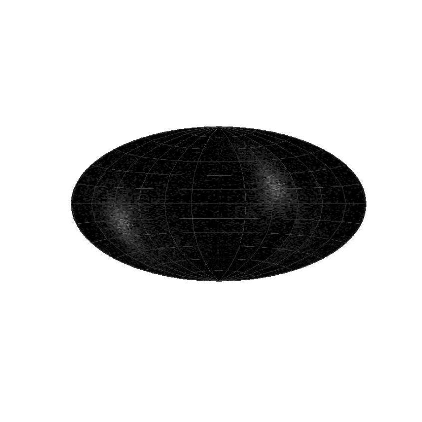
Figure 2: Determination of the wave’s direction using the method of independent bars the presence of Gaussian noise with $SNR\sim 8$. The transducers used are numbers 1, 2, 3, 4 and 6 in Table LABEL:angulosit).

With the above equations we compute the direction of the incoming wave. It results in the same value for each time sample, in the case of a pure (noiseless) signal. In the case of a noisy signal, a distribution around the mean values of the $\beta$ and $\gamma$ angles is found, as we can see from Figures 2 and 3.

III.2 Amplitudes of the polarization states

Using the fact that $\mathbf{e}_{+}\centerdot\mathbf{e}_{+}=2$, $\mathbf{e}_{\times}\centerdot\mathbf{e}_{\times}=2$ and $\mathbf{e}_{+}\centerdot\mathbf{e}_{\times}=0$ we obtain $h_{+}$ and $h_{\times}$ with the aid of equation (8), yielding

$$h_{+}= (\cos^{2}\beta\cos^{2}\gamma-\sin^{2}\gamma)h_{11}+\sin 2\gamma(1+\cos^{2}\beta)h_{12}-\sin 2\beta\cos\gamma h_{13}+$$

$$(\cos^{2}\beta\sin^{2}\gamma-\cos^{2}\gamma)h_{22}-\sin 2\beta\sin\gamma h_{23}+\sin^{2}\beta h_{33},$$

$$h_{\times}= -\cos\beta\sin 2\gamma h_{11}+2\cos\beta\cos 2\gamma h_{12}+2\sin\beta\sin\gamma h_{13}$$

$$+\cos\beta\sin 2\gamma h_{22}-2\sin\beta\cos\gamma h_{23}.$$

Once these amplitudes are known other quantities can be calculated. One of them is the polarization angle, $\Psi$, through the relation

$$\tan(2\psi(t))=\frac{h_{x}(t)}{h_{+}(t)}.$$

However, this parameter is actually not relevant for gravitational wave detection purposes since it is just an arbitrary angle between the wave x axis and an axis where the wave has only the instantaneous plus polarization, $h_{+}$.

On the other hand, important information can be obtained from the difference between the polarization phases. This can be determined if we analyze the time evolution of the instantaneous polarizations registered in each sample (the polarizations are time dependent). Our ability to determine this phase difference depends on the signal to noise ratio for each particular event sampled. Such time varying analysis is beyond the scope of the present work.

IV Testing the method of independent bars

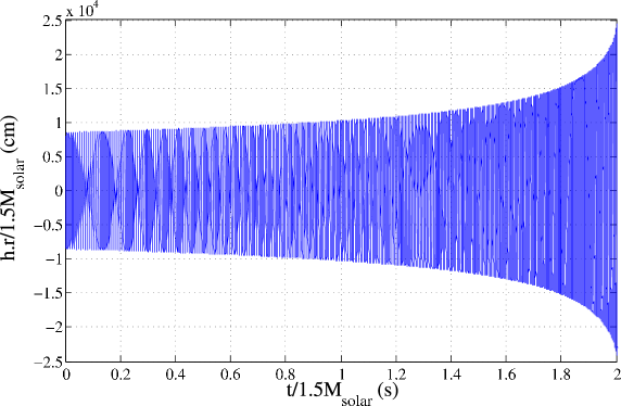
Figure 1: Waveform of a gravitational wave emitted by a binary neutron star-neutron star system near its last stable orbits. The time and amplitude axes are scaled according to the object masses through the multiplication by $M/1.5M_{solar}$, where $M_{solar}$ is the Sun’s mass.

With the objective of testing the efficiency of the method we produced simulated data of the SCHENBERG detector. For the waveform we chose a template from the Laboratory for High Energy Astrophysics (LHEA) of the NASA/GFSCast , one of the three waveforms used by Duez and collaborators Duez et al. (2001a, b) and depicted in Figure 1.

This signal was introduced in a simulator of SCHENBERGCosta (2005), that returns the response of the six two-mode transducers positioned on the detector their positions obeying the truncated icosahedral configurationCosta et al. (2004). The simulation of the detector is possible because its mathematical model is known as well as the mathematical models of its noise sources et al (2004).

Table LABEL:angulosit shows the angles relative to the position of each transducer on the spherical detector. We simulated the transducers’ responses when detector was excited by a wave of the kind shown in Figure 1 arriving at the detector in the direction defined by $\beta=30^{\circ}$ and $\gamma=75^{\circ}$.

Table 1: The angle $\theta_{L}$ is the one that a line L, that passes through the center of a pentagonal face and the origin of the lab frame, makes with the local zenith and $\phi_{L}$ is the angle that L makes with the $x$ axis of the lab frame.

$L$		1	2	3	4	5	6
$\theta_{L}$		$79,1877^{\circ}$	$79,1877^{\circ}$	$79,1877^{\circ}$	$37,3774^{\circ}$	$37,3774^{\circ}$	$37,3774^{\circ}$
$\phi_{L}$		$120^{\circ}$	$240^{\circ}$	$0^{\circ}$	$300^{\circ}$	$180^{\circ}$	$60^{\circ}$

In the SCHENBERG simulator the amplitude signal-to-noise ratio (SNR) was estimated from Thorne as Thorne (1987)

$$SNR=\sqrt{\int_{-\infty}^{\infty}\tilde{W}(f)\frac{|\tilde{h}^{GW}(f)|^{2}}{S_{N}(f)}df},$$ (19)

where $\tilde{W}(f)$ represents the applied filter function (chosen, in the present work, as the function of a pass-band filter). $S_{N}(f)$ is the equivalent noise profile (Gaussian, in this case); it can be obtained from the detector’s output when no useful signal is present, representing the total noise energy in the sphere.

The signal-to-noise used was $SNR\sim 8$ corresponding to a source with behavior as in Figure 1, located approximately $97$ kpc away. It is from this source model that $\tilde{h}^{GW}(f)$ can be obtained.

We used the output of 5 or 6 transducers to test our model, as follows.

IV.1 Case 1: pure signal

Once we had the simulated response of the transducers we calculated the parameters of the gravitational wave using the method of independent bars.

The result obtained with the method for the source’s direction was exactly the same initially imposed: $\beta=30^{\circ}$ and $\gamma=75^{\circ}$. This shows that the method has good accuracy and does not present intrinsic errors.

IV.2 Case 2: signal plus noise

We then tested the method in the presence of noise adding Gaussian noise to the data. To illustrate the results we projected the sphere onto a plane using the Hammer-Aitoff projectionCalabretta and Greisen (2002), where the direction is given by $\theta=90^{\circ}-\beta$ and $\phi=-\gamma$.

Figures 2 and 3 show the source’s direction as found using the method of independent bars for the cases where the data of six or five transducers are used. In those figures the two regions of the sky are marked because there is a natural ambiguity in the determination of the direction by only one detector. If more than one detector is used then there is a time delay between detections and one can determine whether the wave came from up or down.

As one can verify, the smaller the the number of transducers’ data used in the analysis the smaller the precision of the results. In those figures we observe that, for the case in which the data of only five transducers are used, the area of interest is larger than in the case that use the data of all six transducers. This area is equivalent to the error. The numerical results obtained for the method are presented in Table 2.

Table 2: Numerical results obtained with the method of independent bars for the wave’s direction in the case of signal in the presence of noise ($SNR\sim 8$) using five or six transducers’ data. $n$ is the number of the transducers.

$n$	$\beta$	$\gamma$
5	$(27.2\pm 7.1)^{\circ}$	$(78.7\pm 5.3)^{\circ}$
6	$(28.1\pm 4.2)^{\circ}$	$(75.3\pm 2.9)^{\circ}$

The values presented in this Table were obtained simulating the wave’s incidence 50 times and then calculating the average and the standard deviation of the results.

We have verified the efficiency of the method of independent bars in determining a source’s direction. Another important result is to show the equivalence between the method of independent bars and mode channels model Merkowitz and Johnson (1997). This will be done in the next section.

V Equivalence between the method of independent bars and the mode channels model

In order to show the equivalence between the mathod of independent bars and mode channels model, we must write the transducer’s tensor (eqs. 3 and 5) in its trace-free form:

$$D_{ij}=({\mathbf{n}}\otimes{\mathbf{n}})_{ij}-\frac{1}{3}\delta_{ij},$$

where the term $\frac{1}{3}\delta_{ij}$ ensures the property of tracelessness of the tensor.

Each component of the matrix ${\mathbf{D}}$ (eq. 11) is a function of the angles $\theta_{L}$ and $\phi_{L}$ that informs the position of each transducer. When we impose the trace-free condition on the tensor $D_{ij}$, all this functions can be written as a combination of real spherical harmonics of second order. Therefore the matricial system can be written as

$$\left[\begin{array}[]{c}R^{1}\cr R^{2}\cr R^{3}\cr R^{4}\cr R^{5}\cr R^{6}\end{array}\right]=\frac{1}{2}\sqrt{\frac{16\pi}{15}}\begin{bmatrix}Y_{1}^{1}&Y_{2}^{1}&Y_{3}^{1}&Y_{4}^{1}&Y_{5}^{1}\cr Y_{1}^{2}&Y_{2}^{2}&Y_{3}^{2}&Y_{4}^{2}&Y_{5}^{2}\cr Y_{1}^{3}&Y_{2}^{3}&Y_{2}^{3}&Y_{4}^{3}&Y_{5}^{3}\cr Y_{1}^{4}&Y_{2}^{4}&Y_{3}^{4}&Y_{4}^{4}&Y_{5}^{4}\cr Y_{1}^{5}&Y_{2}^{5}&Y_{3}^{5}&Y_{4}^{5}&Y_{5}^{5}\cr Y_{1}^{6}&Y_{2}^{6}&Y_{3}^{6}&Y_{4}^{6}&Y_{5}^{6}\cr\end{bmatrix}\left[\begin{array}[]{c}h_{1}\cr h_{2}\cr h_{3}\cr h_{4}\cr h_{5}\cr\end{array}\right],$$ (20)

where $h_{m}$ are the quadrupolar representation of the gravitational waves. In Appendix A we shown the details of this calculation.

When the transducer are positioned according to the truncated icosahedral configuration the matrix of the real spherical harmonics $\mathbf{Y}$ is the transpose of the model matrix ${\mathbf{B}}^{T}_{6\times 5}$ proposed by Merkowitz and JohnsonJohnson and Merkowitz (1993b). In compact notation equation (20) can be written as

$${\mathbf{R}}=\frac{1}{2}\sqrt{\frac{16\pi}{15}}{\mathbf{B}}^{T}_{6\times 5}{\mathbf{h}}.$$ (21)

Using a property of the model matrixMerkowitz and Johnson (1997):

$${\mathbf{B}}_{5\times 6}{\mathbf{B}}^{T}_{6\times 5}=\frac{3}{2\pi}{\mathbf{I}},$$ (22)

we obtain:

$${\mathbf{h}}=\sqrt{\frac{5\pi}{3}}{\mathbf{B}}_{5\times 6}{\mathbf{R}},$$ (23)

or, in explicit form:

$$\left[\begin{array}[]{c}h_{1}\cr h_{2}\cr h_{3}\cr h_{4}\cr h_{5}\cr\end{array}\right]=\sqrt{\frac{5\pi}{3}}\begin{bmatrix}Y_{1}^{1}&Y_{1}^{2}&Y_{1}^{3}&Y_{1}^{4}&Y_{1}^{5}&Y_{1}^{6}\cr Y_{2}^{1}&Y_{2}^{2}&Y_{2}^{3}&Y_{2}^{4}&Y_{2}^{5}&Y_{2}^{6}\cr Y_{3}^{1}&Y_{3}^{2}&Y_{3}^{3}&Y_{3}^{4}&Y_{3}^{5}&Y_{3}^{6}\cr Y_{4}^{1}&Y_{4}^{2}&Y_{4}^{3}&Y_{4}^{4}&Y_{4}^{5}&Y_{4}^{6}\cr Y_{5}^{1}&Y_{5}^{2}&Y_{5}^{3}&Y_{5}^{4}&Y_{5}^{5}&Y_{5}^{6}\cr\end{bmatrix}\left[\begin{array}[]{c}R^{1}\cr R^{2}\cr R^{3}\cr R^{4}\cr R^{5}\cr R^{6}\end{array}\right].$$ (24)

This result, obtained with the independent bars method, coincides with the one found with the mode channels model. Therefore, if the transducers are in a truncated icosahedron configuration the two models are equivalent.

On the other hand, it is worth stressing that even if the transducers are not in this special configuration the inverse problem can be solved using the independent bars model.

VI Summary

The main objective of this work was to show the details of the analytical construction of the method of independent bars and its efficiency in the determination of the relevant parameters of gravitational waves detected by spherical detector, namely: the two angles that determine the source’s position in the sky and the amplitudes of the two polarization states as functions of time.

As can be seen from the results, the method of independent bars is efficient for the solution of the inverse problem. First we tested the method in the noiseless case and we verified that it does not present intrinsic errors, being thus an exact method. Then we tested the method adding Gaussian noise to the data, as can be seen in Figures 2 and 3.

A major advantage of the method of independent bars is its generality, since it does not depend on the specific transducers’ configuration. The fact that $\mathbf{D}$ is a square matrix facilitates the inversion of the system’s equation, the only requirement being that the matrix is non-singular.

Therefore, the usefulness of this method is evident. For instance, in the absence of any transducer coupled to the spherical detector the mode channels modelMerkowitz and Johnson (1997) does not work. This happens because the truncated icosahedron configuration is lost. However, the independent bars method still works under this condition. We are currently investigating ways to solve the inverse problem with three transducers. We have already got some preliminary results that will appear in a future paper.

In this work we have actually shown that the method of the independent bars is a generalization of the mode channels model. The matrix $\mathbf{D}$ can be written in terms of the real spherical harmonics. In this case, if the transducers’ positions obey the truncated icosahedron configuration we verified that $\mathbf{D}$ is the model matrix $\mathbf{B}_{5\times 6}$ multiplied by a constant.

Finally, we point out that this method can be used for the solution of the inverse problem in a network of bar antennas, as long as a common reference frame is chosen and time delays are accounted for.

Appendix A

Each component of the matrix (11) is a function of the angles $\theta$ and $\phi$ that inform the position of each transducer. The $D$ functions can be written as combinations of the real spherical harmonics as follows:

$$D_{11}^{L} =\frac{1}{2}\left(\sqrt{\frac{16\pi}{15}}Y_{1}^{L}-\sqrt{\frac{16\pi}{45}}Y_{5}^{L}\right),$$

$$D_{12}^{L} =-\frac{1}{2}\sqrt{\frac{16\pi}{15}}Y_{2}^{L},$$

$$D_{13}^{L} =\frac{1}{2}\sqrt{\frac{16\pi}{15}}Y_{3}^{L},$$

$$D_{22}^{L} =-\frac{1}{2}\left(\sqrt{\frac{16\pi}{15}}Y_{1}^{L}+\sqrt{\frac{16\pi}{45}}Y_{5}^{L}\right),$$

$$D_{23}^{L} =-\frac{1}{2}\sqrt{\frac{16\pi}{15}}Y_{4}^{L},$$

$$D_{33}^{L} =\sqrt{\frac{16\pi}{45}}Y_{5}^{L}.$$

Here the $Y_{m}^{L}$ are defined as functions of the spherical harmonics of second order $Y^{L}_{2,n}$ Zhou and Michelson (1994):

$$Y_{1}^{L} =\frac{i}{\sqrt{2}}\left(Y_{2,2}^{L}+Y_{2,-2}^{L}\right),$$

$$Y_{2}^{L} =\frac{1}{\sqrt{2}}\left(Y_{2,-2}^{L}-Y_{2,2}^{L}\right),$$

$$Y_{3}^{L} =\frac{i}{\sqrt{2}}\left(Y_{2,1}^{L}+Y_{2,-1}^{L}\right),$$

$$Y_{4}^{L} =\frac{1}{\sqrt{2}}\left(Y_{2,-1}^{L}-Y_{2,1}^{L}\right),$$

$$Y_{5}^{L} =Y_{2,0}^{L}.$$

Equation (10) can be written in terms of the real spherical harmonics:

$$R^{L}=\frac{1}{2}\sqrt{\frac{16\pi}{15}}\left[Y_{1}^{L}\left(\frac{h_{11}-h_{22}}{2}\right)+Y_{2}^{L}h_{12}+Y_{3}^{L}h_{13}+Y_{4}^{L}h_{23}+\frac{\sqrt{3}}{2}Y_{5}^{L}\right],$$

In a more compact form this reads

$$R^{L}=\frac{1}{2}\sqrt{\frac{16\pi}{15}}\sum^{5}_{1}Y_{m}^{L}h_{m},$$ (27)

where the $h_{m}$ are the quadrupolar representation of the gravitational wave:

$$\begin{array}[]{cc}h_{1}=&\left(\frac{h_{11}-h_{22}}{2}\right),\\ h_{2}=&h_{12},\\ h_{3}=&h_{13},\\ h_{4}=&h_{23},\\ h_{5}=&\frac{\sqrt{3}}{2}h_{33}.\end{array}$$

Therefore the matricial system of the equation (10) takes the form:

$$\left[\begin{array}[]{c}R^{1}\cr R^{2}\cr R^{3}\cr R^{4}\cr R^{5}\cr R^{6}\end{array}\right]=\frac{1}{2}\sqrt{\frac{16\pi}{15}}\begin{bmatrix}Y_{1}^{1}&Y_{2}^{1}&Y_{3}^{1}&Y_{4}^{1}&Y_{5}^{1}\cr Y_{1}^{2}&Y_{2}^{2}&Y_{3}^{2}&Y_{4}^{2}&Y_{5}^{2}\cr Y_{1}^{3}&Y_{2}^{3}&Y_{2}^{3}&Y_{4}^{3}&Y_{5}^{3}\cr Y_{1}^{4}&Y_{2}^{4}&Y_{3}^{4}&Y_{4}^{4}&Y_{5}^{4}\cr Y_{1}^{5}&Y_{2}^{5}&Y_{3}^{5}&Y_{4}^{5}&Y_{5}^{5}\cr Y_{1}^{6}&Y_{2}^{6}&Y_{3}^{6}&Y_{4}^{6}&Y_{5}^{6}\cr\end{bmatrix}\left[\begin{array}[]{c}h_{1}\cr h_{2}\cr h_{3}\cr h_{4}\cr h_{5}\cr\end{array}\right],$$

which is the same used as equation (20).

Appendix B

We want to show in this appendix that equation (2) can be written in terms of the transducer’s response. First we notice that the potential of the tidal force density caused for the passage of a gravitational wave is

$$\phi({\bf x},t)=\sum_{j,k}\frac{1}{2}\rho x_{j}\ddot{h}_{jk}(t)x_{k},$$

where $\rho$ is the mass density and $x_{i}$ is the coordinate location. The term $x_{i}$ represents a vector for the position so it can be written of the following form:

$$x_{i}=\epsilon n_{i},$$

where $\epsilon$ is the amplitude of the vector and $n_{i}$ is represent the unit vector of the position vector. Replacing $x_{i}$ in the equation we get

$$\phi({\bf x},t)=\sum_{j,k}\frac{1}{2}\epsilon^{2}\rho n_{j}\ddot{h}_{jk}(t)n_{k},$$

which can be written in the form

$$\phi({\bf x},t)=\sum_{j,k}\frac{1}{2}\epsilon^{2}\rho\frac{\partial^{2}}{\partial t^{2}}\left(h_{jk}(t)n_{j}n_{k}\right).$$

We have then the contraction of two tensors: the wave’s tensor $h_{ij}$ and a directionality tensor that characterizes the plan in which the states of polarization of the gravitational wave act. We can impose the traceless condition in $n_{i}n_{j}$ adding the term $-\frac{1}{3}\delta_{ij}$. Therefore the equation assumes the form:

$$\phi({\bf x},t)=\sum_{j,k}\frac{1}{2}\epsilon^{2}\rho\frac{\partial^{2}}{\partial t^{2}}\left(h_{jk}(t)\left(n_{j}n_{k}-\frac{1}{3}\delta_{jk}\right)\right),$$

where the term $\left(n_{j}n_{k}-\frac{1}{3}\delta_{jk}\right)$ is the transducer’s tensor of the equation (3). Therefore we can write

$$\phi({\bf x},t)=\sum_{j,k}\frac{1}{2}\epsilon^{2}\rho\frac{\partial^{2}}{\partial t^{2}}\left(h_{jk}(t)D_{jk}\right),$$

or in a more summarized form:

$$\phi({\bf x},t)=\frac{1}{2}\epsilon^{2}\rho\ddot{\mathcal{R}},$$

where $\mathcal{R}$ is the transducer’s response of the equation (1). Using this equation we can write:

$$\phi({\bf x},t)=\sqrt{\frac{4\pi}{15}}\epsilon^{2}\rho\sum_{m}\ddot{h}_{m}(t)Y_{m}.$$

Figure 3: Determination of the wave’s direction uning the method of independent bars in the presence of Gaussian noise with $SNR\sim 8$. The six transducers are positioned according to the truncated icosahedro configuration shown in Table LABEL:angulosit.

References

Weber (1960)
J. A. Weber,
Phys. Rev. D 12,
306 (1960).
Johnson and Merkowitz (1993a)
F. Johnson and
S. Merkowitz,
Phys. Rev. Lett. 70,
2367 (1993a).
Magalhães
et al. (1997a)
N. S. Magalhães,
O. D. Aguiar,
W. W. Johnson,
and C. Frajuca,
Gen. Relat. Grav 29,
1511 (1997a),
and references therein.
Magalhães et al. (1995)
N. S. Magalhães,
W. W. Johnson,
C. Frajuca, and
O. D. Aguiar,
MNRAS 274, 670
(1995).
Aguiar et al (2008)
O. D. Aguiar et al,
Class. Quantum Grav. 25,
114042 (2008).
Merkowitz and Johnson (1997)
S. Merkowitz and
W. Johnson,
Phys. Rev. D 56,
7513 (1997).
Costa and Aguiar (2006)
C. Costa and
O. D. Aguiar, in
Journal of Physics:Conferences Series
(Sixth Edoardo Aamaldi conference on gravitational
waves, Okinawa, Japan, 2006),
vol. 32, pp. 18–22.
Merkowitz
et al. (1999a)
S. M. Merkowitz,
J. A. Lobo, and
M. A. Serrano,
Class. Quantum Grav. 16,
3035 (1999a),
and references therein.
Dhurandar and Tinto (1988)
S. V. Dhurandar
and M. Tinto,
Mon. Not. astron. Soc. 234,
663 (1988).
Newman and Penrose (1962)
E. T. Newman and
R. Penrose,
J. Math. Phys. 3,
566 (1962).
Lenzi et al (2008)
C. H. Lenzi et al,
Gen. Relat. Grav. 40,
183 (2008).
Merkowitz (1998)
S. M. Merkowitz,
Phys. Rev. D 58,
062002 (1998).
Merkowitz
et al. (1999b)
S. M. Merkowitz,
J. A. Lobo, and
M. A. Serrano,
Class. Quantum Grav. 16,
3035 (1999b).
aes et al. (1997)
N. S. M. aes,
W. W. Johnson,
C. Frajuca, and
O. D. Aguiar,
The Astroph. Jour 475,
462 (1997).
Magalhães
et al. (1997b)
N. S. Magalhães,
W. W. Johnson,
C. Frajuca, and
O. D. Aguiar,
The Astroph. Jour. 475,
462 (1997b).
(16)
The AstroGravS “Astrophysical Gravitational-Waves Sources
Archive”: http://astrogras.gsfc.nasa.gov/docs/catalog.htm.
Duez et al. (2001a)
M. D. Duez,
T. W. Baumgarte,
S. L. Shapiro,
M. Shibata, and
K. Uryu,
Phys. Rev. D 65,
024016 (2001a).
Duez et al. (2001b)
M. D. Duez,
T. W. Baumgarte,
and S. L.
Shapiro, Phys. Rev. D
63, 084030
(2001b).
Costa (2005)
C. A. Costa, Ph.D. thesis,
INPE, São José dos Campos
(2005), (in Portuguese).
Costa et al. (2004)
C. A. Costa,
O. D. Aguiar,
and N. S.
Magalhães, Class. Quantum Grav.
21, S827 (2004).
et al (2004)
C. F. et al,
CQG 21, 1107
(2004).
Thorne (1987)
K. S. Thorne,
300 Years of Gravitation
(Cambridge Univ. Press, Cambridge,
1987).
Calabretta and Greisen (2002)
M. R. Calabretta
and E. W.
Greisen, A&A
395, 1077 (2002).
Johnson and Merkowitz (1993b)
W. W. Johnson and
S. M. Merkowitz,
Phys. Rev. Letters 70,
2367 (1993b).
Zhou and Michelson (1994)
C. Z. Zhou and
P. F. Michelson,
Phys. Rev. D 51,
2517 (1994).