Folding $3$-noncrossing RNA pseudoknot structures

Abstract.

In this paper we present a selfcontained analysis and description of the novel ab initio folding algorithm cross, which generates the minimum free energy (mfe), $3$-noncrossing, $\sigma$-canonical RNA structure. Here an RNA structure is $3$-noncrossing if it does not contain more than three mutually crossing arcs and $\sigma$-canonical, if each of its stacks has size greater or equal than $\sigma$. Our notion of mfe-structure is based on a specific concept of pseudoknots and respective loop-based energy parameters. The algorithm decomposes into three parts: the first is the inductive construction of motifs and shadows, the second is the generation of the skeleta-trees rooted in irreducible shadows and the third is the saturation of skeleta via context dependent dynamic programming routines.

1. Introduction and background

In this paper we introduce the ab initio folding algorithm cross which folds RNA (ribonucleic acid) sequences [49] into pseudoknot structures. We give a selfcontained presentation and analysis of cross, whose source code is publicly available at

$${\tt www.combinatorics.cn/cbpc/cross.html}$$

Supplementary material, such as detailed description of the loop-energies and all implementation details can be found at the above web-site. Let us begin by providing some background on RNA sequences and structures. An RNA molecule is firstly described by its primary sequence, a linear string composed by the four nucleotides A, G, U and C together with the Watson-Crick (A-U, G-C) and (U-G) base pairing rules. Secondly, RNA, structurally less constrained than its chemical relative DNA, folds into helical structures by pairing the nucleotides and thereby lowering their minimum free energy, see Fig.1

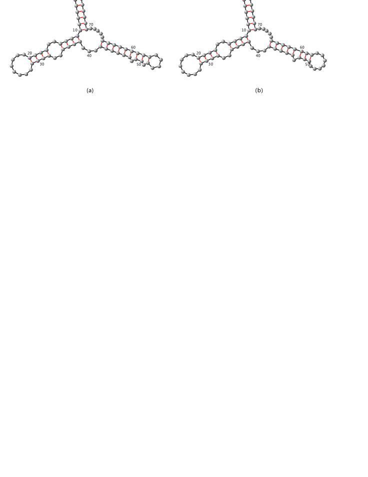
Figure 1. The phenylalanine tRNA (re)visited: (a) represents the structure of phenylalanine tRNA, as folded by ViennaRNA [17, 19]. (b) shows the phenylalanine structure as folded by cross with minimum stack size $3$. Note that cross does not contain any stack which size $\leq 3$, therefore (b) is different from (a) slightly in $48$ to $60$.

Accordingly, RNA exhibits a variety of 3-dimensional structural configurations, the so called tertiary structures, determining the functionality of the molecule. Besides the noncrossing base pairings found in RNA secondary structures there exist further types of nucleotide interactions [53]. These bonds are called pseudoknots and occur in functional RNA like for instance RNAseP [30] as well as ribosomal RNA [29]. Indeed, RNA exhibits a diversity of biochemical capabilities [2], proved by the discovery of catalytic RNAs, or ribozymes [30], in 1981. Like proteins, RNA is capable of catalyzing reactions whereas transfer RNA acts as a messenger between DNA and protein.

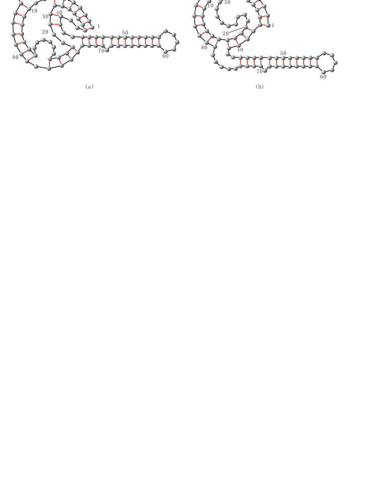
Figure 2. The HDV-pseudoknot structure: (a) displays the structure as folded by Rivas and Eddy’s algorithm [40]. (b) shows the structure as folded by cross with minimum stack size $3$.

In light of these RNA functionalities the question of RNA structure prediction appears to be of relevance. The first mfe-folding algorithms for RNA secondary structure are due to [12, 28, 8] and the first DP folding routines for secondary structures were given by Waterman et al. [46, 52, 54, 34], predicting the loop-based mfe-secondary structure [49] in $O(n^{3})$-time and $O(n^{2})$-space. The general problem of RNA structure prediction under the widely used thermodynamic model is known to be NP-complete when the structures considered include arbitrary pseudoknots [31]. There exist however, polynomial time folding algorithms, capable of the energy based prediction of certain pseudoknots: Rivas et.al. [40], Uemura et.al. [50], Akutsu [3] and Lyngsø[31]. In the following we shall use the term pseudoknot synonymous with cross-serial dependencies between pairs of nucleotides [45, 4]. As for the ab initio folding of pseudoknot RNA, we find the following two paradigms: Rivas and Eddy’s [40] gap-matrix variant of Waterman’s DP-folding routine for secondary structures [46, 51, 20, 52, 34], maximum weighted matching algorithms [11, 13] and the latter taylored for pseudoknot prediction [5, 47]. The former method folds into a somewhat “mysterious” class of pseudoknots [41] in polynomial time. Algorithms along these lines have been developed by Dirks and Pierce [9], Reeder and Giegerich [36] and Ren et al. [39]. Additional ideas for pseudoknot folding involve the iterated loop matching approach [42] and the sampling of RNA structures via the Markov-chain Monte-Carlo method [33].

Let us now have a closer look at the DP-paradim by means of analyzing the algorithm of Rivas and Eddy [40, 41, 10]. In the course of our analysis we shall make two key observations: first, DP algorithms inevitably produce arbitrarily high crossing numbers, see Tab.1 and second that not all $3$-noncrossing RNA structures can be generated by dynamic programming algorithms–at least not with the implemented truncations.

$k$	$2$	$3$	$4$	$5$
growth rate	2.6180	4.7913	6.8541	8.8875
$k$	$6$	$7$	$8$	$9$
growth rate	10.9083	12.9226	14.9330	16.9410

Table 1. The exponential growth rates of $k$-noncrossing RNA structures (minimum arc-length greater or equal than two).

The generation of high crossing numbers is insofar problematic as it implies a very large output class. Already for $k=4$, i.e. for RNA structures exhibiting three mutually crossing arcs, we have an exponential growth rate of $6.8541$–a growth rate exceeding that of the number of natural sequences. In other words, only for an exponentially small fraction of these structures we will find a sequence folding into it. Remarkably, this growth rate appears to grow linearly in $k$, see Tab.1. Any type of study, along the lines of [44, 23, 43, 38, 18, 15, 16], which is based on such an algorithm, is purely computational and does not allow to deduce generic properties in the sense of [48].

Let us define now the non gap-matrices ($vx$, $wx$) and the gap-matrices ($whx$, $vhx$, $zhx$ and $yhx$). [40, 35] The non gap-matrices, $vx$ and $wx$ are two triangular $n\times n$ matrices, where $vx(i,j)$ is the score of the best folding between position $i$ and $j$, provided that $i,j$ are paired to each other and whereas $wx(i,j)$ is the score of the best folding between the position $i$ and $j$, regardless of whether $i,j$ are paired or not. See Tab.2.

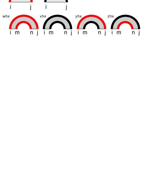
Figure 3. Non gap- and gap-matrices. The non gap-matrices $wx$, $vx$ and gap-matrices $whx$, $vhx$, $yhx$ and $zhx$.

The gap-matrices are pairs of matrices, $\alpha hx(i,j;r,s)$, where $\alpha=w,v,z,y$, are the scores of the best folding depending on the relation between the positions $i,j$ and the relation between positions $r,s$, respectively, see Fig.3.

Matrices	$(i,j)$	$(r,s)$	Matrices	$(i,j)$	$(r,s)$
$whx(i,j;r,s)$	unknown	unknown	$vhx(i,j;r,s)$	paired	paired
$yhx(i,j;r,s)$	unknown	paired	$zhx(i,j;r,s)$	paired	unknown

Table 2. Table shows the gap-matrix $whx$, $vhx$, $yhx$ and $zhx$.

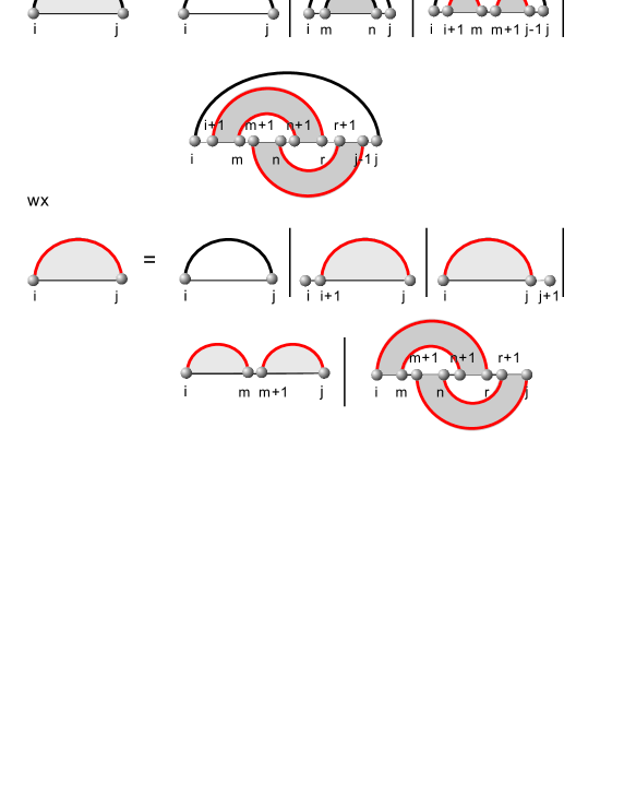
Figure 4. The basic recursions: recursion for $vx$ and $wx$ truncated at $O(whx+whx+whx)$ in Rivas and Eddy’s algorithm.

The key idea in Rivas and Eddy’s algorithm is to use gap-matrices as a generalization of the non gap-matrices $wx$ and $vx$. In particular, both concepts merge for $r=s-1$, where we have for any $i\leq r\leq j$

(1.1) $$whx(i,j;r,r+1) = wx(i,j)$$

(1.2) $$zhx(i,j;r,r+1) = vx(i,j).$$

In Fig.4 we illustrate the recursion for $wx$ and $vx$ in the pseudoknot algorithm truncated at $O(whx+whx+whx)$. We can draw the following two conclusions:
$\bullet$ by design–the inductive formation of gap-matrices generates arbitrarily high numbers of mutually crossing arcs, see Fig.5.
$\bullet$ nonplanar, $3$-noncrossing pseudoknots cannot be generated by inductively forming pairs of gap-matrices, see Fig.6.
In order to avoid any confusion: gap-matrices can and will generate nonplanar arc configurations, however, they can only facilitate this via increasing the crossing number, Fig.5. Fig.6 makes evident that the situation is more complex: nonplanarity is not tied to crossings–there are planar as well as nonplanar $3$-noncrossing structures.

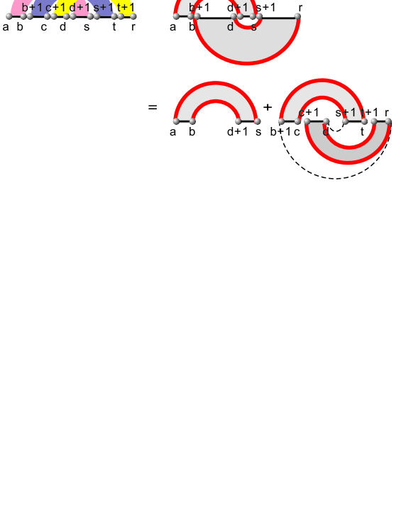
Figure 5. No control over crossings: Here we show how to build a $4$-noncrossing RNA pseudoknot with gap-matrices. Iterating the formation of gap-matrices will produce higher and higher crossings.

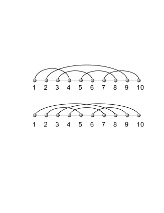
Figure 6. Two nonplanar, $3$-noncrossing RNA structures, which cannot be generated by pairs of gap-matrices.

2. Specifying an output: $k$-noncrossing, canonical RNA structures

The previous section showed that, for RNA pseudoknot structures, DP-algorithms fold into an uncontrollably large set of structures. This phenomenon is in vast contrast to the situation for RNA secondary structures. The standard DP-routine cannot produce any crossings, whence they a priori produce secondary structures. We now follow in the footsteps of Waterman by generalizing his strategy for the case of secondary structures to pseudoknot structures. Accordingly, the first step is to specify a combinatorial output class. To this end we shall provide some basic facts on a particular representation of RNA structures.

A $k$-noncrossing diagram is a labeled graph over the vertex set $[n]$ with vertex degrees $\leq 1$, represented by drawing its vertices $1,\ldots,n$ in a horizontal line and its arcs $(i,j)$, where $i<j$, in the upper half-plane, containing at most $k-1$ mutually crossing arcs. The vertices and arcs correspond to nucleotides and Watson-Crick (A-U, G-C) and (U-G) base pairs, respectively. Diagrams have the following three key parameters: the maximum number of mutually crossing arcs, $k-1$, the minimum arc-length, $\lambda$ and minimum stack-length, $\sigma$ ($(k,\lambda,\sigma)$-diagrams). The length of an arc $(i,j)$ is given by $j-i$ and a stack of length $\sigma$ is the sequence of “parallel“ arcs of the form

(2.1) $$((i,j),(i+1,j-1),\ldots,(i+(\sigma-1),j-(\sigma-1))),$$

see Fig.7.

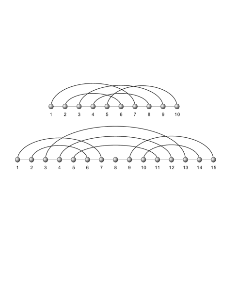
Figure 7. $k$-noncrossing diagrams: we display a $4$-noncrossing, arc-length $\lambda\geq 4$ and $\sigma\geq 1$ (upper) and $3$-noncrossing, $\lambda\geq 4$ and $\sigma\geq 2$ (lower) diagram.

We call an arc of length $\lambda$ a $\lambda$-arc.

We are now in position to specify the output-set. We shall consider RNA pseudoknot structures that are $3$-noncrossing, $\sigma\geq 3$-canonical and have a minimum arc-length $\lambda\geq 4$. The $3$-noncrossing property is mostly for algorithmic convenience and the generalization to higher crossing numbers represents not a major obstacle. We consider $3$-canonical structures, i.e. those in which each stack has length at least three, since we are interested in minimum free energy structures. Finally, the minimum arc-length of four is a result of biophysical constraints. Accordingly, we shall identify pseudoknot RNA structures with $\langle k,4,\sigma\rangle$-diagrams and refer to them simply as $\langle k,\sigma\rangle$-structures, implicitly assuming the minimum arc-length $\lambda\geq 4$. In Fig.8

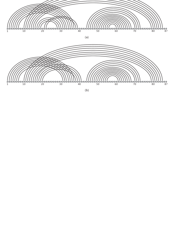
Figure 8. The HDV-virus pseudoknot structures as folded by cross (b). This structure differs from the natural structure displyed in (a) [1] by exactly seven base pairs.

we present a particular $3$-noncrossing, $3$-canonical RNA structure: the HDV-virus as folded by cross.

We next present some of the combinatorics of $\langle 3,\sigma\rangle$-structures. Let $\mathsf{T}_{k,\sigma}^{[4]}$ denote the number of $k$-noncrossing, $\sigma$-canonical RNA structures over $[n]$. The generating function,

$$\mathbf{T}_{k,\sigma}^{[4]}(z)=\sum_{n\geq 0}\mathsf{T}_{k,\sigma}^{[4]}(n)z^{n}\quad k,\sigma\geq 3$$

of $k$-noncrossing, $\sigma$-canonical RNA structures has been obtained in [32]. This function is closely related to $\mathbf{F}_{k}(z)=\sum_{n}f_{k}(2n,0)z^{2n}$, the ordinary generating function of $k$-noncrossing matchings. Beyond functional equations implied directly by the reflection-principle [14], the following asymptotic formula has been derived [27]

(2.2) $$\forall k\in\mathbb{N},\quad f_{k}(2n,0)\sim c_{k}n^{-((k-1)^{2}+(k-1)/2)}(2(k-1))^{2n},\quad c_{k}>0.$$

Setting

$$w_{0}(x)=\frac{x^{2\sigma-2}}{1-x^{2}+x^{2\sigma}}\quad\text{\rm and}\quad v_{0}(x)=1-x+w_{0}(x)x^{2}+w_{0}(x)x^{3}+w_{0}(x)x^{4}$$

we can now state

Theorem 2.1.

Let $k,\sigma\in\mathbb{N}$, where $k,\sigma\geq 3$, $x$ is an indeterminate and $\rho_{k}$ the dominant, positive real singularity of $\mathbf{F}_{k}(z)$. Then $\mathbf{T}_{k,\sigma}^{[4]}(x)$, the generating function of $\langle k,\sigma\rangle$-structures, is given by

(2.3) $$\mathbf{T}_{k,\sigma}^{[4]}(x)=\frac{1}{v_{0}(x)}\mathbf{F}_{k}\left(\frac{\sqrt{w_{0}(x)}x}{v_{0}(x)}\right).$$

Furthermore, the asymptotic formula

(2.4) $$\mathbf{T}_{k,\sigma}^{[4]}(n)\sim c_{k}n^{-(k-1)^{2}-(k-1)/2}\left(\frac{1}{\gamma_{k,\sigma}^{[4]}}\right)^{n},\ \quad\ \text{\rm for}\quad k=3,4,\ldots,9.$$

holds, where $\gamma_{k,\sigma}^{[4]}$ is the minimal positive real solution of the equation $\frac{\sqrt{w_{0}(x)}x}{v_{0}(x)}=\rho_{k}$.

Theorem $1$ implies exact enumeration results as well as an array of exponential growth rates indexed by $k$ and $\sigma$. The latter are presented in Tab.3 and are of relevance in the context of the asymptotic analysis of the algorithm.

$k$	$3$	$4$	$5$	$6$	$7$	$8$	$9$
$\sigma=3$	$2.0348$	$2.2644$	$2.4432$	$2.5932$	$2.7243$	$2.8414$	$2.9480$
$\sigma=4$	$1.7898$	$1.9370$	$2.0488$	$2.1407$	$2.2198$	$2.2896$	$2.3523$
$\sigma=5$	$1.6465$	$1.7532$	$1.8330$	$1.8979$	$1.9532$	$2.0016$	$2.0449$
$\sigma=6$	$1.5515$	$1.6345$	$1.6960$	$1.7457$	$1.7877$	$1.8243$	$1.8569$
$\sigma=7$	$1.4834$	$1.5510$	$1.6008$	$1.6408$	$1.6745$	$1.7038$	$1.7297$
$\sigma=8$	$1.4319$	$1.4888$	$1.5305$	$1.5639$	$1.5919$	$1.6162$	$1.6376$
$\sigma=9$	$1.3915$	$1.4405$	$1.4763$	$1.5049$	$1.5288$	$1.5494$	$1.5677$

Table 3. Exponential growth rates of $\langle k,\sigma\rangle$-structures.

In addition, Tab.3 shows that $3$-noncrossing, $\sigma$-canonical RNA structures have remarkably moderate growth rates. $\sigma$-canonical structures with higher crossing numbers exhibit also moderate growth rates, indicating that generalizations of the current implementation of cross from $k=3$ to $k=4$ or $5$ are feasible.

3. Loops, motifs and shadows

Suppose we are given a $\langle 3,\sigma\rangle$-structure, $S$. Let $\alpha$ be an $S$-arc and denote the set of $S$-arcs that cross $\beta$ by $\mathscr{A}_{S}(\beta)$. Clearly we have

(3.1) $$\beta\in\mathscr{A}_{S}(\alpha)\quad\Longleftrightarrow\quad\alpha\in\mathscr{A}_{S}(\beta).$$

An arc $\alpha\in\mathscr{A}_{S}(\beta)$ is called a minimal, $\beta$-crossing if there exists no $\alpha^{\prime}\in\mathscr{A}_{S}(\beta)$ such that $\alpha^{\prime}\prec\alpha$. Note that $\alpha\in\mathscr{A}_{S}(\beta)$ can be minimal $\beta$-crossing, while $\beta$ is not minimal $\alpha$-crossing. We call a pair of crossing arcs $(\alpha,\beta)$ balanced, if $\alpha$ is minimal, $\beta$-crossing and $\beta$ is minimal $\alpha$-crossing, respectively. $3$-noncrossing diagrams exhibit the following four basic loop-types $3$-noncrossing diagrams:

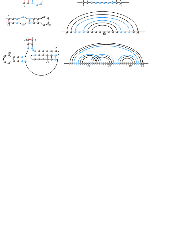
Figure 9. The standard loop-types: hairpin-loop (top), interior-loop (middle) and multi-loop (bottom). These represent all loop-types that occur in RNA secondary structures.

(1) a hairpin-loop, being a pair

$$((i,j),[i+1,j-1])$$

where $(i,j)$ is an arc and $[i,j]$ is an interval, i.e. a sequence of consecutive vertices $(i,i+1,\dots,j-1,j)$.
(2) an interior-loop, being a sequence

$$((i_{1},j_{1}),[i_{1}+1,i_{2}-1],(i_{2},j_{2}),[j_{2}+1,j_{1}-1]),$$

where $(i_{2},j_{2})$ is nested in $(i_{1},j_{1})$.
(3) a multi-loop, see Fig.9, being a sequence

$$((i_{1},j_{1}),[i_{1}+1,\omega_{1}-1],S_{\omega_{1}}^{\tau_{1}},[\tau_{1}+1,\omega_{2}-1],S_{\omega_{2}}^{\tau_{2}},\dots)$$

where $S_{\omega_{h}}^{\tau_{h}}$ denotes a pseudoknot structure over $[\omega_{h},\tau_{h}]$ (i.e. nested in $(i_{1},j_{1})$) and subject to the following condition: if all $S_{\omega_{h}}^{\tau_{h}}=(\omega_{h},\tau_{h})$, i.e. all substructures are simply arcs, for all $h$, then $h\geq 2$.

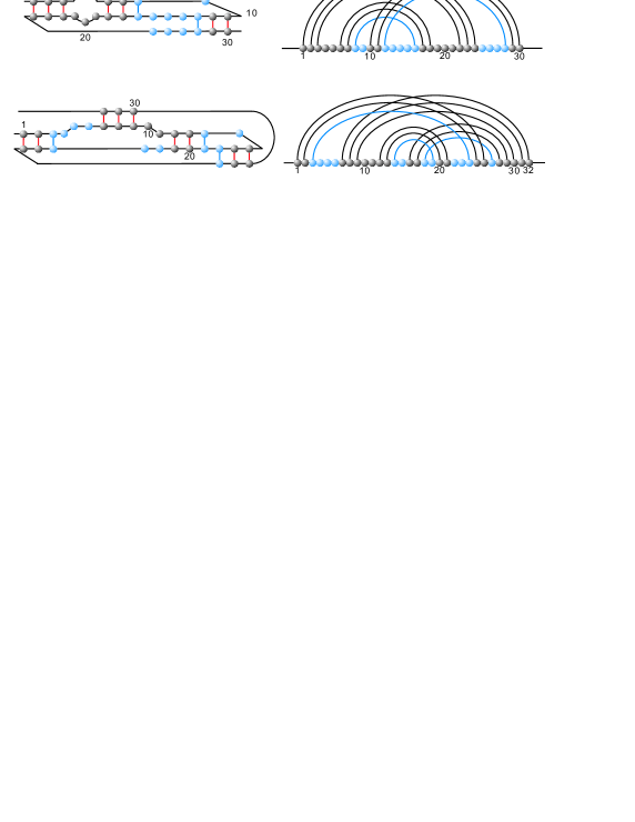
Figure 10. Pseudoknots: we display a balanced (top) and an unbalanced pseudoknot (bottom). The latter contains the stack over $(3,24)$, which is minimal for the arc $(9,30)$, which is not contained in the pseudoknot.

We finally define pseudokont-loops:
(4) a pseudoknot, see Fig.10, consists of the following data:
(P1) a set of arcs

$$P=\left\{(i_{1},j_{1}),(i_{2},j_{2}),\dots,(i_{t},j_{t})\right\},$$

where $i_{1}=\min\{i_{s}\}$ and $j_{t}=\max\{j_{s}\}$, such that
(i) the diagram induced by the arc-set $P$ is irreducible, i.e. the line-graph of $P$ is connected and
(ii) for each $(i_{s},j_{s})\in P$ there exists some arc $\beta$ (not necessarily contained in $P$) such that $(i_{s},j_{s})$ is minimal $\beta$-crossing.
(P2) all vertices $i_{1}<r<j_{t}$, not contained in hairpin-, interior- or multi-loops.
We call a pseudoknot balanced if its arc-set can be decomposed into pairs of balanced arcs.

3.1. Motifs and shadows

Let $\prec$ denote the partial order over the set of arcs (written as $(i,j),\ i<j)$ of a $k$-noncrossing diagram, given by

(3.2) $$(i_{1},j_{1})\prec(i_{2},j_{2})\ \Longleftrightarrow\ i_{2}<i_{1}\ \wedge\ j_{1}<j_{2}.$$

A $k$-noncrossing core is a $k$-noncrossing diagram without any two arcs of the form $(i,j),\ (i+1,j-1)$. Any $k$-noncrossing RNA structure, $S$ has a unique $k$-noncrossing core, $c(S)$ [25], obtained in two steps: first one identifies all arcs contained in stacks, inducing a contracted diagram and secondly one relabels the vertices.

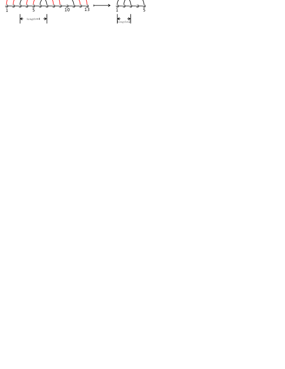
Figure 11. Core-structures: A structure, $S$, (lhs) is mapped into its core $c(S)$ (rhs). Clearly $S$ has arc-length $\geq 4$ and as a consequence of the collapse of the stack $((4,13),(5,12),(6,11))$ (the red arcs are being removed) into the arc $(2,5)$. $c(S)$ contains the arc $(1,3)$. This arc becomes, after relabeling, a $2$-arc.

Note that the core-map does in general not preserve arc-length.

Definition 1.

(Motif) A $\langle k,\sigma\rangle$-motif, $\mathfrak{m}$, is a $\langle k,\sigma\rangle$-structure over $[n]$, having the following properties:
(M1) $\mathfrak{m}$ has a nonnesting core.
(M2) All $\mathfrak{m}$-arcs are contained in stacks of length exactly $\sigma\geq 3$ and length $\lambda\geq 4$.
The set of all motifs is denoted by $\mathbb{M}^{\sigma}_{k}(n)$ and we set $\mu^{*}_{k,\sigma}(n)=|\mathbb{M}^{\sigma}_{k}(n)|$.

Property (M1) is obviously equivalent to: all arcs of the core, $c(\mathfrak{m})$, are $\prec$-maximal.

Let $S$ be a $\langle 3,\sigma\rangle$-structure. We call two $k$-noncrossing diagrams $\delta_{1},\delta_{2}$ adjacent if and only if $\delta_{2}$ is derived by selecting a pair of isolated $\delta_{1}$-vertices, $i<j$ such that $(i-1,j+1)$ is a $\delta_{1}$-arc. With respect to this notion of adjacency the set of $k$-noncrossing diagrams over $[n]$ becomes a directed graph, which we denote by $\mathscr{G}_{k}(n)$.

Definition 2.

(Shadow) A shadow of $S$ is a $\mathscr{G}_{k}(n)$-vertex connected to $S$ by a $\mathscr{G}_{k}(n)$-path.

Intuitively speaking, a shadow is derived by extending the stacks of a structure from top to bottom.

Theorem 3.1.

Suppose $k,\sigma\geq 2$.
(a) Any $k$-noncrossing, $\sigma$-canonical RNA structure corresponds to a unique sequence of shadows.
(b) Any $\langle 3,\sigma\rangle$-structure has a unique loop-decomposition.

Proof.

Ad (a). Suppose $S$ is an arbitrary $\langle k,\sigma\rangle$-structure over $[n]$. We prove the theorem by induction on the number of $S$-arcs. We consider the set of $\prec$-maximal elements, $S^{*}=\{(i,j)\mid(i,j)\ \text{\rm is $\prec$-maximal}\}.$ Clearly, $S^{*}$ induces a unique $\langle k,\sigma\rangle$-motif, $\mathfrak{m}_{k,\sigma}(S)$, contained in $S$. Indeed, since $S$ is by assumption $\sigma$-canonical, each $S^{*}$-arc occurs in a stack of size $\geq\sigma$. By definition, any $S$-arc which is contained in a stack containing an (unique) $S^{*}$-arc is an arc of an unique shadow, $\overline{\mathfrak{m}}_{k,\sigma}(S)$. Removing all arcs contained in $\overline{\mathfrak{m}}_{k,\sigma}(S)$ the remaining diagram is still $k$-noncrossing and $\sigma$-canonical. To see this it suffices to observe that any $S$-arc not contained in $\overline{\mathfrak{m}}_{k,\sigma}(S)$ is contained in a stack of size $\geq\sigma$ not containing any $\overline{\mathfrak{m}}_{k,\sigma}(S)$-arcs. Assertion (a) follows now by induction on the number of arcs.
Ad (b). Let $c(S)$ be the core of $S$. We shall color the $c(S)$-arcs, $\alpha=(i,j)$, as follows:
Case (1): $\mathscr{A}_{c(S)}(\alpha)\neq\varnothing$.
Since $c(S)$ is a $3$-noncrossing diagram, we have for any two $(i,j),(i^{\prime},j^{\prime})\in\mathscr{A}_{c(S)}(\beta)$, either $(i,j)\prec(i^{\prime},j^{\prime})$ or $j<i^{\prime}$. Therefore for any $\beta\in\mathscr{A}_{c(S)}(\alpha)$ there exists an unique $\prec$-minimal arc $\alpha^{*}∗\in\mathscr{A}_{c(S)}(\beta)$ that is nested in $\alpha$. If there exists some $\beta$ for which $\alpha=\alpha^{*}(\beta)$ holds, i.e. $\alpha$ itself is minimal in $\mathscr{A}_{c(S)}(\beta)$, then we color $\alpha$ red. In other words, red arcs are minimal with respect to some crossing $\beta$. Otherwise, for any $\beta\in\mathscr{A}_{c(S)}(\alpha)$ there exists some $\alpha^{*}(\beta)\prec\alpha$. If $\alpha^{*}(\beta)$ is the unique $\prec$-maximal substructure nested in $\alpha$, then we color $\alpha$ green and blue, otherwise.
Case (2): $\mathscr{A}_{c(S)}(\alpha)=\varnothing$, i.e. $\alpha$ is noncrossing in $c(S)$.
If there exists no $c(S)$-arc $\alpha^{\prime}\prec\alpha$, then we color $\alpha$ purple, if there exists exactly one maximal $c(S)$-arc $\alpha^{\prime}\prec\alpha$, we color $\alpha$ green and blue, otherwise. It follows now by induction on the number of $c(S)$-arcs that this procedure generates a well defined arc-coloring. Let $i\in[n]$ be a vertex. We assign to $i$ either the color of the minimal non-red $c(S)$-arc $(r,s)$ for which $r<i<s$ holds, or red if there exist only red $c(S)$-arcs, $(r,s)$ with $r<i<s$ and black, otherwise. By construction, this induces a vertex-arc coloring with the property of correctly identifying all hairpin- (purple arcs and vertices), interior- (green arcs and vertices), multi- (blue arcs and vertices) and pseudoknot (red arcs and vertices). ∎

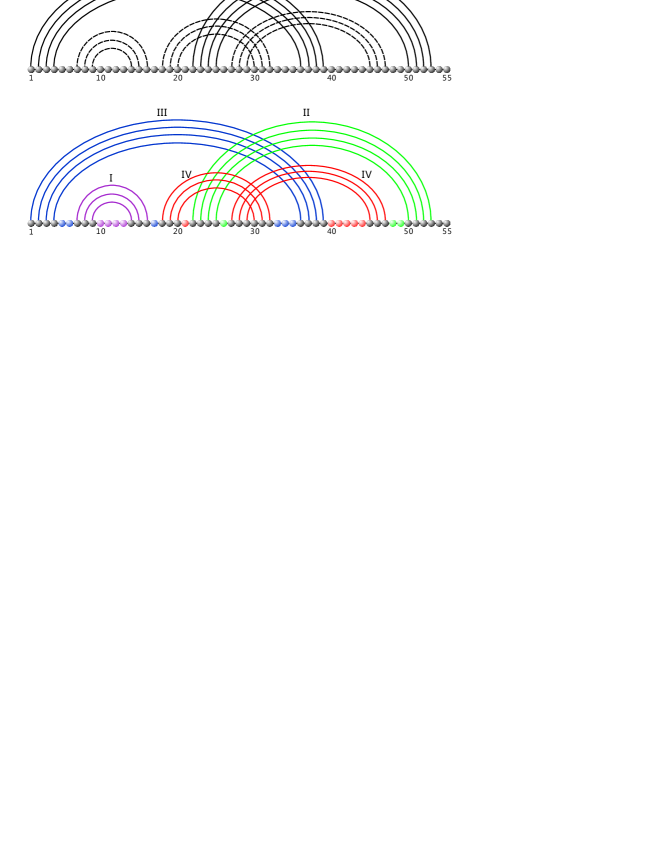
Figure 12. Shadows and loops: we give the sequence of shadows (top) and the loop-decomposition (below) illustrating Theorem 3.1. Here I (purple) is a hairpin-loop, II (green) represents an interior-loop, III (blue) is a multi-loop and finally IV (red) is a (balanced) pseudoknot.

In Fig.12 we show how these decompositions work.

4. Phase I: motif-generation

The first step in cross consists in creating some kind of shelling of a $3$-noncrossing, canonical structure via motifs. One key idea in cross is the identification of motifs as building blocks. The key point here is that, despite the fact that motifs exhibit complicated crossings, they can be inductively generated. This is remarkable and a result of considering the “dual” of a motif which turns out to be a restricted Motzkin-path. The latter is obtained via the bijection of Proposition 4.1 between crossing and nesting arcs.

A Motzkin-path is composed by up-, down- and horizontal-steps. It starts at the origin, stays in the upper halfplane and ends on the $x$-axis. Let ${\rm Mo}_{k}^{\sigma}(n)$ denote the following set of Motzkin-paths:
(a) the paths have height $\leq\sigma(k-1)$
(b) all up- and down-steps come only in sequences of length $\sigma$
(c) all plateaux at height $\sigma$ have length $\geq 3$.
Let $\mu_{k-1,\sigma}(n)$ denote the number of Motzkin-paths of length $n$ that (a’) have height $\leq\sigma(k-2)$, (b’) up- and down-steps come only in sequences of length $\sigma$. We set for arbitrary $k,\sigma\geq 2$

$$G^{*}_{k,\sigma}(z) = \sum_{n\geq 0}\mu^{*}_{k,\sigma}(n)z^{n}$$

$$G_{k-1,\sigma}(z) = \sum_{n\geq 0}\mu_{k-1,\sigma}(n)z^{n}$$

$$G_{1,\sigma}(z) = \frac{1}{1-z}.$$

Now we are in position to give the main result of this section:

Proposition 4.1.

Suppose $k,\sigma\geq 2$, then the following assertions hold:
(a) There exists a bijection

(4.1) $$\beta:\mathbb{M}_{k}^{\sigma}(n)\longrightarrow\text{\rm Mo}_{k}^{\sigma}(n).$$

(b) We have the following recurrence equations

(4.2) $$\mu^{*}_{k,\sigma}(n) = \mu^{*}_{k,\sigma}(n-1)+\sum_{s=0}^{n-(2\sigma+3)}\mu_{k-1}(n-2\sigma-s)\mu^{*}_{k,\sigma}(s)\quad\text{\rm for}\ n>2\sigma$$

(4.3) $$\mu_{k,\sigma}(n) = \mu_{k,\sigma}(n-1)+\sum_{s=0}^{n-2\sigma}\mu_{k-1}(n-2\sigma-s)\mu_{k,\sigma}(s)\qquad\text{\rm for}\ n>2\sigma-1.$$

where $\mu^{*}_{k,\sigma}(n)=1$ for $0\leq n\leq 2\sigma$ and $\mu_{k-1,\sigma}(n)=1$ for $0\leq n\leq 2\sigma-1$.
(c) We have the following formula for the generating functions

(4.4) $$G^{*}_{k,\sigma}(z) = \frac{1}{1-z-z^{2\sigma}(G_{k-1,\sigma}(z)-(z^{2}+z+1))}$$

(4.5) $$G_{k-1,\sigma}(z) = \frac{1}{1-z-z^{2\sigma}G_{k-2,\sigma}(z)}.$$

and, in particular, for $k=3$ we have the following asymptotic formula

(4.6) $$\mu^{*}_{3,\sigma}(n)\sim c_{\sigma}\left(\frac{1}{\zeta_{\sigma}}\right)^{n},$$

where $c_{\sigma}$ and $\zeta_{\sigma}^{-1}$ are given by Tab.4.

$\sigma$	$2$	$3$	$4$	$5$	$6$	$7$
$\zeta^{-1}_{\sigma}$	1.7424	1.5457	1.4397	1.3721	1.3247	1.2894
$c_{\sigma}$	0.1077	0.0948	0.0879	0.0840	0.0804	0.0780

Table 4. The exponential growth rates of $\mu^{*}_{3,\sigma}(n)$

Proof.

Let $\mathfrak{m}$ be a $\langle k,\sigma\rangle$-motif. We construct the bijection $\beta$ as follows: reading the vertex labels of $\mathfrak{m}$ in increasing order we map each $\sigma$-tuple of origins and termini into a $\sigma$-tuple of up-steps and down-steps, respectively. Furthermore isolated points are mapped into horizontal-steps. The resulting paths are by construction Motzkin-paths of height $\leq\sigma(k-1)$. Since motifs have arcs of length $\geq 4$ the paths have at height $\sigma$ plateaux of length $\geq 3$. In addition we have $\sigma$-tuples of up- and down-steps. Therefore $\beta$ is well defined. To see that $\beta$ is bijective we construct its inverse explicitly. Consider an element $\zeta\in\text{\rm Mo}^{\sigma}_{k}(n)$. We shall pair $\sigma$-tuples of up-steps and down-steps as follows: starting from left to right we pair the first up-step with the first down-step tuple and proceed inductively, see Fig.13.

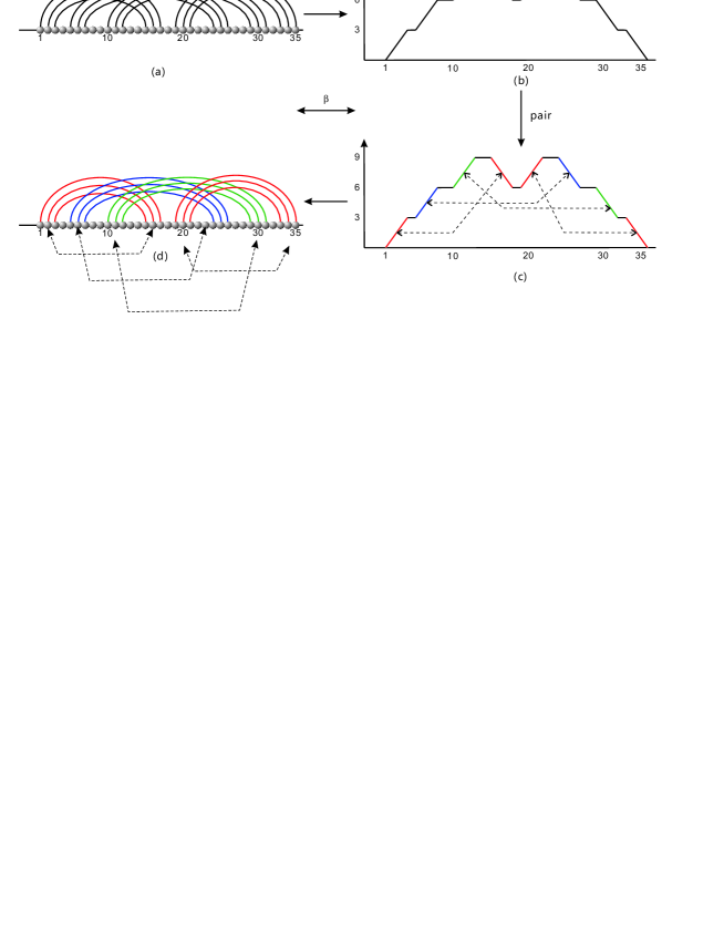
Figure 13. The bijection $\beta$: First we have a map from (a) to (b). Then we pair the $\sigma$-tuples of up-steps and down-steps, see the vertical map from (b) to (c). The so derived pairs, see the horizontal map from (c) to (d), allow to reconstruct the original motif.

It is clear from the definition of Motzkin-paths that this pairing procedure is well defined. Each such pair

$$((u_{i},u_{i+1},\ldots,u_{i+\sigma},(d_{j},d_{j+1},\ldots,j_{j+\sigma}))$$

corresponds uniquely to the sequence of arcs $((i+\sigma,j),\ldots,(i,j+\sigma))$ from which we can conclude that $\zeta$ induces a unique $\sigma$-canonical diagram, $\delta_{\zeta}$ over $[n]$. Furthermore $\delta_{\zeta}$ has by construction a nonnesting core. A diagram contains a $k$-crossing if and only if it contains a sequence of arcs $(i_{1},j_{1}),\ldots,(i_{k},j_{k})$ such that $i_{1}<i_{2}<\cdots<i_{k}<j_{1}<j_{2}<\cdots<j_{k}$. Therefore $\delta_{\zeta}$ is $k$-noncrossing if and only if its underlying path $\zeta$ has height $<\sigma k$. We immediately derive $\beta(\delta_{\zeta})=\zeta$, whence $\beta$ is a bijection. Using the Motzkin-path interpretation we immediately observe that $\text{\rm Mo}_{k}^{\sigma}(n)$-paths can be constructed recursively from paths that start with a horizontal-step or an up-step, respectively. The recursions eq. (4.2) and eq. (4.3) and the generating functions of eq. (4.4) and eq. (4.5) are straightforwardly derived. As for the particular case $G^{*}_{3,\sigma}(z)$, we have

(4.7) $$G^{*}_{3,\sigma}(z)=\frac{1}{1-z-z^{2\sigma}\left[\frac{1}{1-z-z^{2\sigma}[\frac{1}{1-z}]}-(z^{2}+z+1)\right]}.$$

The unique dominant, real singularities of $G^{*}_{3,\sigma}(z)$ are simple poles, denoted by $\zeta_{\sigma}$. Being a rational function, $G^{*}_{k,\sigma}(z)$ admits a partial fraction expansion

$$G^{*}_{k,\sigma}(z)=H(z)+\sum_{(\zeta,r)}\frac{c_{(\zeta,r)}}{(\zeta-z)^{r}}$$

and eq. (4.6) follows in view of

(4.8) $$[z^{n}]\frac{1}{\zeta-z}=\frac{1}{\zeta}[z^{n}]\frac{1}{1-z/\zeta}=\frac{1}{\zeta}{n\choose 0}\left(\frac{1}{\zeta}\right)^{n}=\left(\frac{1}{\zeta}\right)^{n+1}.$$

∎

5. Phase II: the skeleta-tree

In this section we enter the second phase of cross. What will happen here, is that each irreducible shadow, generated during the first phase described in Section 4, gives rise to a tree of skeleta. The intuition behind this construction is that each tree-vertex, i.e. each skeleton, represents a maximal “non-inductive” arc configuration. This does not mean that a skeleton contains all crossings arcs of the final structure, but all further crossings are derived by adding independent substructures. In other words: their energy contributions are additive.

A skeleton, $S$, is a $3$-noncrossing structure whose core has no noncrossing arcs, i.e. for any arc $\alpha$ we have $\mathscr{A}_{S}(\alpha)\neq\varnothing$, see Fig.14. In addition, in a skeleton over the segment $\{i,i+1,\dots,j-1,j\}$, $S_{i,j}$, the positions $i$ and $j$ are paired. Recall that an interval is a sequence of consecutive, unpaired bases $(i,i+1,\cdots,j)$, where $i-1$ and $j+1$ are paired. Furthermore, recall that a stack of length $\sigma$ (see eq. (2.1)) is a sequence of parallel arcs $((i,j),(i+1,j-1),\ldots,(i+(\sigma-1),j-(\sigma-1)))$, which we write as $(i,j,\sigma)$. Note that $\sigma\geq\sigma_{0}$, where $\sigma_{0}$ is the minimum stack length of the structure, see Fig.14. An irreducible shadow over $\{i,i+1,\dots,j-1,j\}$ is denoted by $IS_{i,j}$. It is a particular skeleton, i.e. a skeleton in which there are no nested arcs.

Remark 1.

In our implementation of cross, the number of stacks of an irreducible shadow is an input parameter. As default we set its maximum value to be three.

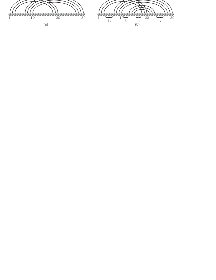
Figure 14. Irreducible shadows and skeleta: an irreducible shadow (a), containing the stack $(1,20,3)$ and $(7,30,4)$. (b) A skeleton drawn with its four induced intervals $I_{1},I_{2},I_{3},I_{4}$.

We are now in position to construct the skeleta-tree. Suppose we are given a $3$-noncrossing skeleton, $S$. We label the $S$-intervals $\{I_{1},\dots,I_{m}\}$ from left to right and consider pairs $(S,r)$, where $r$ is an integer $1\leq r\leq m-1$. Given a pair $(S,r)$ we construct new pairs $(S^{\prime},r^{\prime})$ where $r^{\prime}\geq r$ as follows: we replace a pair of intervals $(I_{p},I_{q})$, $i\in I_{p},j\in I_{q}$, $i\geq r$ by the stack $\alpha=(i,j,\sigma)$, subject to the following conditions

• $S^{\prime}$ is a $3$-noncrossing skeleton

• $(i+\sigma-1,j-\sigma+1)$ is a minimal element in $(S^{\prime},\prec)$

• $r^{\prime}$ is the label of the first paired base preceding the interval $I_{p}$.

• $i-1$ and $j+1$ are not paired to each other.

Fig.15 displays the two basic scenarios via which stacks are being inserted.

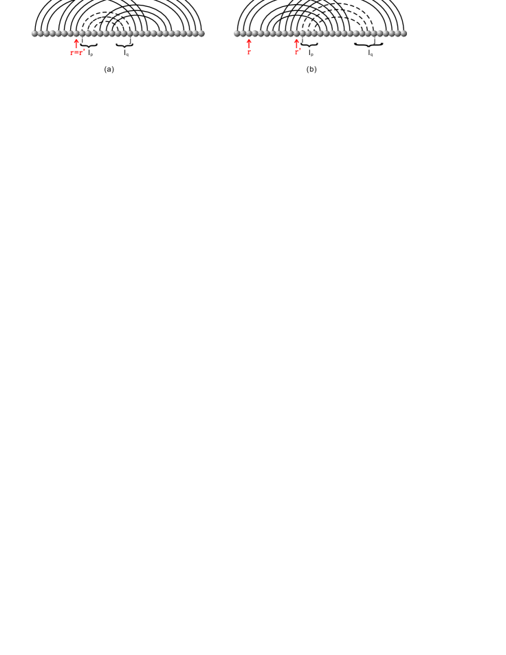
Figure 15. Stack-insertion: if the origin of the inserted stack $(i,j,\sigma)$ is smaller than that of its predecessor (a), then $r=r^{\prime}$. Paraphrasing the situation we can express this as “left-insertion” freezes the index $r$. Accordingly, (b) showcases the “right-insertion”, with its induced shift of the indices $r\mapsto r^{\prime}$, both indices are drawn in red.

We refer to the above procedure as $(i,j,\sigma)$-insertion and formally express it via

(5.1) $$(S,r)\Rightarrow_{(i,j,\sigma)}(S^{\prime},r^{\prime}).$$

Given a pair $(S,r)$ subsequent insertions induce a directed graph, $G_{(S,r)}$, whose vertices are pairs $(S^{\prime},r^{\prime})$ and whose (directed) arcs are given by

(5.2) $$((S,r),(S^{\prime},r^{\prime})),\quad\text{\rm where}\quad(S,r)\Rightarrow_{(i,j,\sigma)}(S^{\prime},r^{\prime}).$$

Remark 2.

Note that the algorithm checks whether $(i,j,\sigma)$ can be added, i.e. (1) the bases $\{i,i+1,\cdots,i+\sigma-1,j-\sigma+1,\cdots,j-1,j\}$ are indeed unpaired and (2) $(i-1,j+1)$ is not a base pair. The second property guarantees that the core of the stack $(i,j,\sigma)$ is an arc in the core of $S^{\prime}$.

We proceed by showing that $G_{(S,r)}$ is in fact a tree. In other words, the insertion-procedure is an unambiguous grammar.

Proposition 5.1.

Let $T_{1}=\{S\mid\exists\,r;\,(S,r)\in T\}$ and $S_{0}$ be a $3$-noncrossing skeleton.
(a) $G_{(S_{0},r_{0})}$ is a tree and for any two different vertices $(S^{\prime}_{1},r^{\prime}_{1})$ and $(S^{\prime}_{2},r^{\prime}_{2})$ in $G_{(S,r_{0})}$, we have $S^{\prime}_{1}\neq S^{\prime}_{2}$.
(b) For $k>3$, the graph morphism $\pi\colon\mathbb{T}\longrightarrow\mathbb{T}_{1}$, given by $\pi((S,r))=S$ is not bijective.

Remark 3.

For any $k>3$, $G_{(S_{0},r_{0})}$ is a tree. However assertion (b) indicates that it is really a tree of pairs. That means, stack-insertions will in general generate two different pairs with equal first coordinate.

Proof.

We prove assertion (a) by induction on the number of inserted arcs, $\ell$. For $\ell=0$ there is nothing to prove. For $\ell=1$, the pairs $(S,r_{0})$ and $(S^{\prime},r^{\prime})$ differ by exactly one stack, $(i,j,\sigma)$, whence the assertion. Our objective is now to show that for any two $(S_{1}^{\prime},r_{1}^{\prime})$ and $(S^{\prime}_{2},r^{\prime}_{2})$ obtained from the root $(S,r_{0})$ via $\ell$ insertions, $S_{1}^{\prime}\neq S_{2}^{\prime}$ holds. Suppose there exists some $(\tilde{S},\tilde{r})$, such that

(5.3)

If the inserted stacks coincide, we have $(S_{1}^{\prime},r_{1}^{\prime})=(S_{2}^{\prime},r_{2}^{\prime})$ and there is nothing to prove. Otherwise, we obtain $S^{\prime}_{1}\neq S^{\prime}_{2}$, which implies $(S_{1}^{\prime},r_{1}^{\prime})\neq(S_{2}^{\prime},r_{2}^{\prime})$, whence (a). Suppose next, we have the following situation

(5.4)

where the uniqueness of the paths ending at $(S_{1},r_{1})$ and $(S_{2},r_{2})$ is guaranteed by the induction hypothesis. By assumption we have $(S_{1},r_{1})\neq(S_{2},r_{2})$ and $S_{1}$ and $S^{\prime}_{1}$ as well as $S_{2}$ and $S^{\prime}_{2}$ differ by exactly one stack. Again by induction hypothesis, we have $S_{1}\neq S_{2}$, whence

(5.5) $$(S_{1},r_{1})\Rightarrow_{\alpha=(i_{\alpha},j_{\alpha},\sigma_{\alpha})}(S_{1}^{\prime},r_{1}^{\prime}),\ (S_{2},r_{2})\Rightarrow_{\beta=(i_{\beta},j_{\beta},\sigma_{\beta})}(S_{2}^{\prime},r_{2}^{\prime})\quad\text{\rm and}\quad S_{1}\neq S_{2}.$$

We now prove the inductive step by contradition. Suppose we have $S^{\prime}_{1}=S^{\prime}_{2}$, then we can conclude that $\alpha\neq\beta$ and there exists some $(\tilde{S},\tilde{r})$ such that

(5.6)

Indeed, we define $\tilde{S}$ to be the skeleton derived from $(S_{0},r_{0})$ by inserting all $S^{\prime}_{1}$-arcs except of $\alpha,\beta$. It is clear that the skeleton $\tilde{S}$ exists since its stack-set is a subset of the stack-set of $S^{\prime}_{1}$. By construction, $\tilde{S}$ differs from $S_{1}$ and $S_{2}$ via the stacks $\alpha$ and $\beta$, respectively. By induction hypothesis, there exists a unique path from $(S,r_{0})$ to $(\tilde{S},\tilde{r})$, which implies the existence of a unique $\tilde{r}$. Furthermore, by induction hypothesis, the paths from $(S_{0},r_{0})$ to $(S_{1},r_{1})$ and $(S_{2},r_{2})$ are unique and consequently contain $(\tilde{S},\tilde{r})$, whence we have the situation given in eq. (5.6).
As $\alpha$ and $\beta$ are both minimal, without loss of generality we may assume $i_{\alpha}<i_{\beta}$. Let us consider the insertion-path $(\tilde{S},\tilde{r})\Rightarrow_{\beta}(S_{1},r_{1})\Rightarrow_{\alpha}(S_{1}^{\prime},r_{1}^{\prime})$. According to this insertion, we obtain $r_{1}<i_{\alpha}$ and by construction $[r_{1}+1,i_{\beta}-1]$ is an $S_{1}$-interval. If $j_{\alpha}<i_{\beta}$, then $\alpha$ does not cross any arcs in $S^{\prime}_{1}$, which is impossible. If $j_{\alpha}>j_{\beta}$, we arrive at $\beta\prec\alpha$, which contradicts minimality of $\alpha$. Therefore, we have $i_{\beta}<j_{\alpha}<j_{\beta}$, i.e. the arcs $\alpha$ and $\beta$ are crossing. Next we consider $(\tilde{S},\tilde{r})\Rightarrow_{\alpha}(S_{2},r_{2})\Rightarrow_{\beta}(S_{2}^{\prime},r_{2}^{\prime})$. Accordingly, $\alpha$ must be crossed by some $(\tilde{S},\tilde{r})$-stack, say $\gamma=(i_{\gamma},j_{\gamma},\sigma_{\gamma})$. We next put $\gamma$ into the context of the insertion-path $(\tilde{S},\tilde{r})\Rightarrow_{\beta}(S_{1},r_{1})\Rightarrow_{\alpha}(S_{1}^{\prime},r_{1}^{\prime})$ and observe that $\gamma$ necessarily crosses $\beta$. Indeed, otherwise we have the following three scenarios: $i_{\gamma}>j_{\beta}$, $j_{\gamma}\leq r_{1}$ or $i_{\gamma}\leq r_{1},j_{\gamma}>j_{\beta}$. In all three cases $\gamma$ cannot cross $\alpha$ since $i_{\gamma},j_{\gamma}\not\in[r_{1}+1,i_{\beta}-1]$, see Fig.16.

Figure 16. Illustration of the proof of Proposition 5.1. The three different scenarios for a noncrossing $\gamma$, representing stacks by isolated arcs. (a) $j_{\gamma}\leq r_{1}$, (b) $i_{\gamma}>j_{\beta}$ and (c) $i_{\gamma}\leq r_{1}$, $j_{\gamma}>j_{\beta}$.

As a result, $\gamma$ necessarily crosses both stacks: $\alpha$ and $\beta$, which is a contradition to the fact that $S^{\prime}_{1}$ is a $3$-noncrossing skeleton, whence $S^{\prime}_{1}\neq S^{\prime}_{2}$. In particular we obtain $(S^{\prime}_{1},r^{\prime}_{1})\neq(S^{\prime}_{2},r^{\prime}_{2})$, the insertion path is unique and $G_{(S,r_{0})}$ is a tree.
In order to prove (b) we provide via Fig.17 an example, where the implication $(S_{1},r_{1})\neq(S_{2},r_{2})\,\Rightarrow S_{1}\neq S_{2}$ does not hold. Note that $\mathbb{T}_{(S_{0},r_{0})}$ is still a tree. ∎

Next we prove that our unambiguous grammar indeed generates any skeleton, which contains a given irreducible shadow.

Proposition 5.2.

Suppose we are given an irreducible shadow $S_{0}=IS_{i,j}$. Let $\mathbb{T}(S_{0})=G_{(S_{0},0)}$ denote ist skeleton-tree and let $\mathbb{S}(S_{0})$ be the set of all skeleta, that contain $S_{0}$. Then we have

(5.7) $$\mathbb{T}(S_{0})=\mathbb{S}(S_{0}).$$

Proof.

Let $\mathscr{A}_{S}$ denote the set of $S$-arcs. Obviously, for any vertex $(S,r)\in\mathbb{T}(S_{0})$, $S$ is a $3$-noncrossing skeleton such that $\mathscr{A}_{S_{0}}\subseteq\mathscr{A}_{S}$, whence $\mathbb{T}(S_{0})\subseteq\mathbb{S}(S_{0})$ holds. For an arbitrary $3$-noncrossing skeleton $S$, let $\mathscr{A}_{S}^{\text{\rm ne}}$ denote the set of all nested stacks in $S$. Since each arc is either maximal or nested we have $\mathscr{A}_{S}=\mathscr{A}_{S_{0}}\dot{\cup}\mathscr{A}_{S}^{\text{\rm ne}}$. Sorting $\mathscr{A}_{S}^{\text{\rm ne}}$ via the linear ordering of their leftmost paired base, we obtain the sequence $\Sigma=(\alpha_{1},\alpha_{2},\cdots,\alpha_{n})$. We choose the first element $\alpha_{k}\in\Sigma$ which is intersecting $S_{0}$ (not necessarily $\alpha_{1}$). Then we have

(5.8) $$(S_{0},r_{0})\hookrightarrow_{\alpha_{k}}(S_{1},r_{1})$$

where, $S_{1}\in\mathbb{T}(S_{0})$. We proceed inductively, setting $\mathscr{A}_{S}^{\text{\rm ne}}=\mathscr{A}_{S}^{\text{\rm ne}}\setminus\alpha_{k}$ and proceed inductively until $\mathscr{A}_{S}^{\text{\rm ne}}=\varnothing$. By construction, each $S_{k}$ is in $\mathbb{T}(S_{0})$, and $S_{n}=S$. Accordingly, we constructed an insertion-path in $\mathbb{T}(S_{0})$ from $S_{0}$ to $S$, from which $\mathbb{S}(S_{0})\subset\mathbb{T}(S_{0})$ follows. ∎

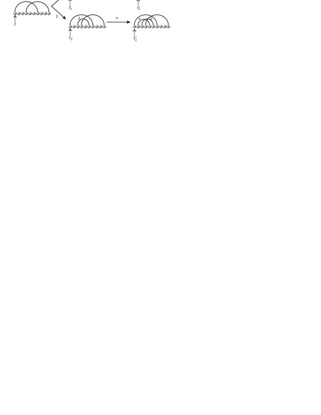
Figure 17. Illustration of assertion (b) of Proposition 5.1: the case $k>3$. While $\mathbb{T}_{(S_{0},r_{0})}$ is still a tree (over pairs), the implication $(S_{1},r_{1})\neq(S_{2},r_{2})\,\Rightarrow S_{1}\neq S_{2}$ does not hold in general.

6. Phase III: Saturation

In this section we discuss the third phase of cross. The skeleta-trees constructed in the second phase organized the non-inductive substructures of an irreducible shadow derived in phase one. The objective of the saturation phase is to inductively “fill” the remaining intervals of a given skeleton with specific substructures. Basically, all routines employed here follow the DP-paradigm. However, we store a vector of structures rather than energies and implement context sensitive DP-routines.

Suppose we are given a skeleta-tree $\mathbb{T}(S_{0})$ with root $S_{0}$. Let the order of $S$, $\omega(S)$, denote the number of $\prec$-maximal $S$-arcs, see Fig.18. Furthermore, let $\Sigma_{i,j}$ and $\Sigma^{[r]}_{i,j}$ be some subset of structures over $\{i,i+1,\dots,j-1,j\}$ and those of order $r$, respectively.

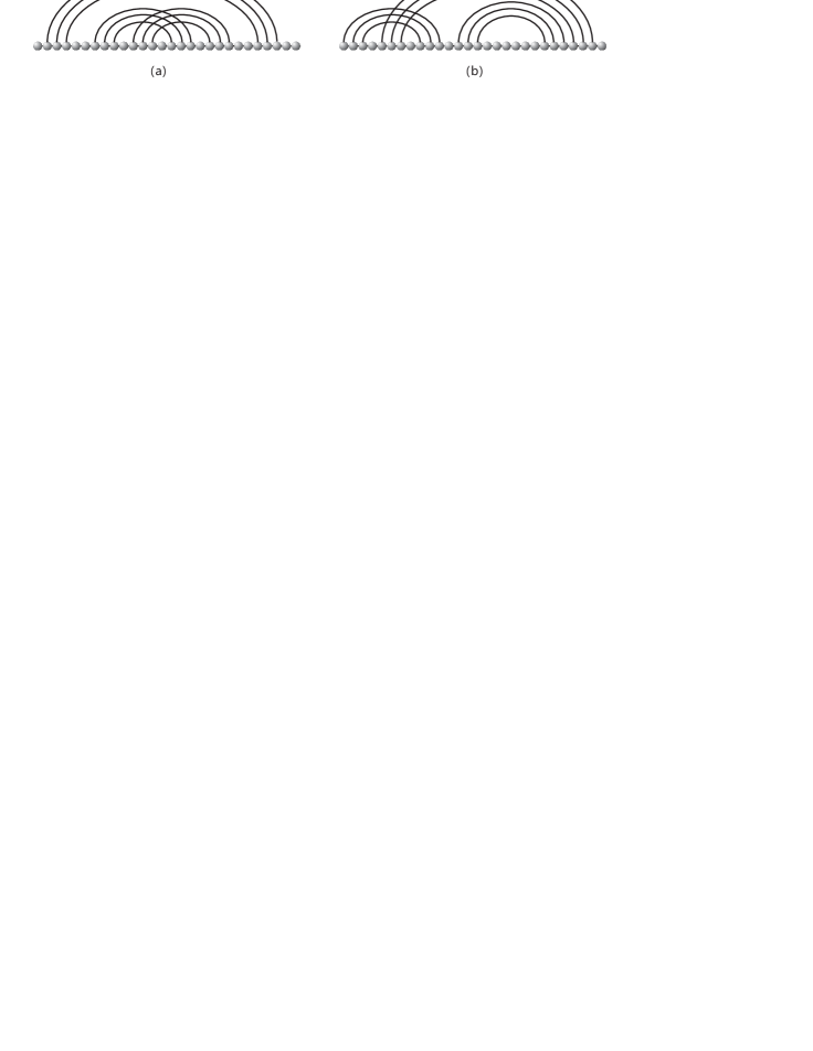
Figure 18. Order: In (a) we display a structure of order one. (b) showcases a structure of order two.

Let $\mathbb{M}_{i,j}$ denote the set of saturated skeleta over $\{i,i+1,\dots,j-1,j\}$ and $OSM(i,j)\in\mathbb{M}_{i,j}$ be a mfe-saturated skeleton. Furthermore, let $OS(i,j)$ be a mfe-structure, which is a union of disjoint $OSM(i_{1},j_{1}),\dots OSM(i_{r},j_{r})$ and unpaired nucleotides. By $OSM^{[x]}(i,j)$ and $OS^{[x]}(i,j)$ we denote the respective $OSM$ and $OS$ structures of order $x$.

Figure 19. $OS$ vers. $OSM$: we display a $OSM(i,j)$ (a), and a $OS(i,j)$ structure (b). The $OS(i,j)$ structure shown in (b) is evidently an union of of the structures $OSM(i,s)$ and $OSM(s+1,j)$ and the unpaired nucleotide at position $i$.

In order to describe the context-sensitive saturation procedure in cross we denote by $OS_{\text{\rm mul}}(i,j)$, $OS_{\text{\rm pk}}(i,j)$ and $OS_{0}(i,j)$, the mfe-structures nested in a multi-loop, pseudoknot and otherwise, respectively.

For a given a skeleton $S_{i,j}$, we specify the mapping $S_{i,j}\mapsto OSM(S_{i,j})$ as follows: suppose $S_{i,j}$ has $n_{1}$ intervals, $I_{1},\dots,I_{n_{1}}$ labelled from left to right. For given interval $I_{r}=[i_{r},j_{r}]$ and $s_{r}\in\Sigma_{i_{r},j_{r}}$ we consider the insertion of $s_{r}$ into $I_{r}$, distinguishing the following four cases:
Case(1). $I_{r}$ is contained in a hairpin-loop.
$\omega(s_{r})=0$. That is we have $s_{r}=\varnothing$. The loop generated by the $s_{r}$-insertion remains obviously a hairpin-loop, i.e. $((i_{r}-1,j_{r}+1),[i_{r},j_{r}]),$ with energy $H(i_{r}-1,j_{r}+1)$.
$\omega(s_{r})=1$. Let $(p,q)$ be the unique, maximal $s_{r}$-arc. Then $s_{r}$-insertion produces the interior-loop

$$((i_{r}-1,j_{r}+1),[i_{r},p-1],(p,q),[q+1,j_{r}]),$$

with energy $I(i_{k}-1,j_{k}+1,p,q)$. Note that $p=i_{r}$ implies $q\neq j_{r}$ and $s_{r}\in OSM_{0}^{[1]}(p,q)$.
$\omega(s_{r})\geq 2$. In this case inserting $s_{r}$ into $I_{r}$ creates a multi-loop in which $s_{r}$ is nested. Then $s_{k}\in OS^{[\geq 2]}_{\text{\rm mul}}$, see Fig.20. Let $\epsilon(s)$ denote the energy of structure $s$. We select the set of all structures $s_{r}$ such that

$$\epsilon(s_{r})=\text{\rm min}\begin{cases}H(i_{r}-1,j_{r}+1)\\ I(i_{r}-1,j_{r}+1,p,q)+\epsilon(OSM_{0}^{[1]}(p,q))\\ \quad\quad\forall i_{r}\leq p<q\leq j_{r}\ \text{\rm and }\ p=i_{r},\Rightarrow q\neq j_{k}\\ M+P_{1}+\epsilon(OS^{[\geq 2]}_{\text{\rm mul}}(i_{r},j_{r})).\end{cases}$$

Here, $M$ is the energy penalty for forming a multi-loop and $P_{1}$ is the energy score of a closing-pair in multi-loop.

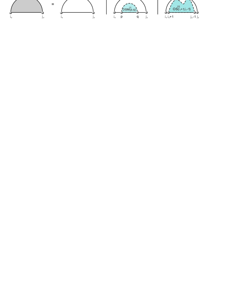
Figure 20. Saturation in hairpin-loops: the interval on the left hand side is filled with substructures $s_{r}$ such that $\omega(s_{r})=0$ (left), $\omega(s_{r})=1$ (middle) or $\omega(s_{r})\geq 2$ (right).

Case(2). $I_{r}$ is contained in a pseudoknot loop.
$\omega(s_{r})=0$. That is we have $s_{r}=\{\varnothing\}$ and the unpaired bases in $I_{r}$ are considered to be contained in a pseudoknot.
$\omega(s_{r})\geq 1$. In this case, $s_{r}$ is a substructure which is nested in a pseudoknot, see Fig.21. As a result our selection criterion is given by

$$\epsilon(s_{r})=\text{\rm min}\begin{cases}(j_{r}-i_{r}+1)\cdot Q_{\text{\rm pk}}\\ \epsilon(OS_{\text{\rm pk}}(i_{r},j_{r})).\end{cases}$$

where $(j_{r}-i_{r}+1)\in\mathbb{N}$ is the number of unpaired bases in $I_{r}$, and $Q_{\text{\rm pk}}$ is the energy score of the unpaired bases in a pseudoknot.

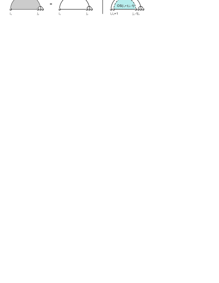
Figure 21. Saturation of interval nested in a pseudoknot.

Case(3). $I_{r}$ is contained in a multi-loop. In analogy to case (2), we distinguish the following cases:
$\omega(s_{r})=0$. That is we have $s_{r}=\{\varnothing\}$. The unpaired bases in $I_{r}$ are considered to be contained in a multi-loop.
$\omega(s_{r})\geq 1$. In this case, $s_{r}$ is a substructure nested in a multi-loop, see Fig.22. Accordingly, we select all structures satisfying

$$\epsilon(s_{r})=\text{\rm min}\begin{cases}(j_{r}-i_{r}+1)\cdot Q_{\text{\rm mul}}\\ \epsilon(OS_{\text{\rm mul}}(i_{r},j_{r})),\end{cases}$$

where $Q_{\text{\rm mul}}$ denotes the energy score of the unpaired bases in a multi-loop.

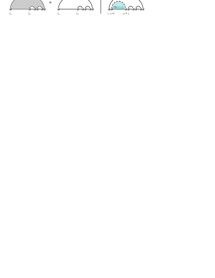
Figure 22. Saturation of an interval contained in a multi-loop.

Case(4) $I_{r}$ is contained in an interior-loop. By construction, the latter is formed by the pair $(I_{r},I_{l})$, where $r<l$. We then select pairs $s_{r}$ in $\Sigma_{i_{r},j_{r}}$ and $s_{l}$ in $\Sigma_{i_{l},j_{l}}$. Note that only the first coordinate of the pair $(I_{r},I_{l})$ is considered.
$\omega(s_{r})=0$ and $\omega(s_{l})=0$. Obviously, in this case the loop formed by $I_{r}$ and $I_{l}$ remains an interior-loop

$$((i_{r}-1,j_{l}+1),[i_{r},j_{r}],(j_{r}+1,i_{l}-1),[i_{l},j_{l}]),$$

whose energy is given by $I(i_{r}-1,j_{l}+1,j_{r}+1,i_{l}-1)$.
$\omega(s_{r})\geq 1$ and $\omega(s_{l})=0$. In this case, $s_{l}=\{\varnothing\}$. $I_{r}$ and $I_{l}$ create a multi-loop, in which $s_{r}$ and the substructure $G_{j_{r}+1,i_{l}-1}$ are nested.
$\omega(s_{r})=0$ and $\omega(s_{l})\geq 1$. Completely analogous to the previous case.
$\omega(s_{r})\geq 1$ and $\omega(s_{l})\geq 1$. In this case, $I_{r}$ and $I_{l}$ create a multi-loop, in which $s_{r}$, $s_{l}$ and $G_{j_{r}+1,i_{l}-1}$ are nested, see Fig.23.
Accordingly, we select all pairs of structures $(s_{r},s_{l})$ satisfying

$$\epsilon(s_{r})+\epsilon(s_{l})=\text{\rm min}\begin{cases}I(i_{r}-1,j_{l}+1,j_{r}+1,i_{l}-1)\\ M+2P_{1}+\epsilon(OS_{\text{\rm mul}}(i_{r},j_{r}))+(j_{l}-i_{l}+1)\cdot Q_{\text{\rm mul}}\\ M+2P_{1}+\epsilon(OS_{\text{\rm mul}}(i_{l},j_{l}))+(j_{k}-i_{k}+1)\cdot Q_{\text{\rm mul}}\\ M+2P_{1}+\epsilon(OS_{\text{\rm mul}}(i_{r},j_{r}))+\epsilon(OS_{\text{\rm mul}}(i_{l},j_{l}))\\ \end{cases}$$

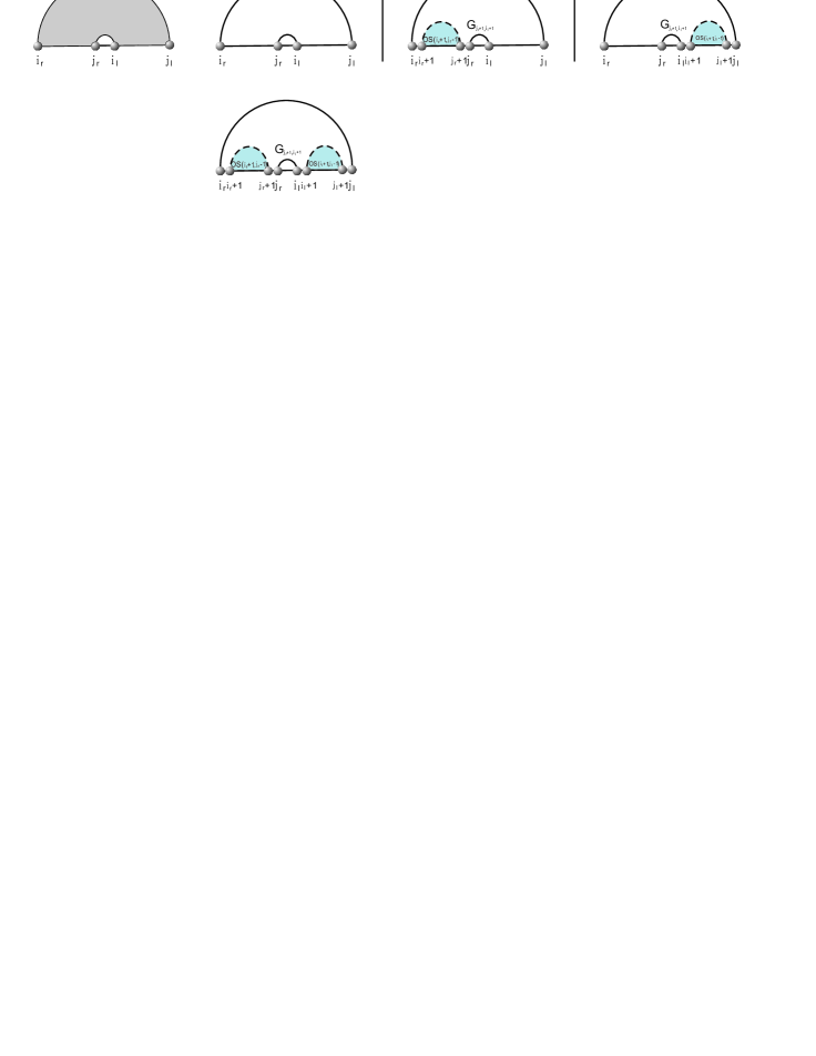
Figure 23. Saturation of an interval contained in an interior-loop, which is obtained by $I_{r}$ and $I_{l}$, where $r<l$.

Accordingly, we inductively saturate all intervals and in case of interior loops interval-pairs and thereby derive $OSM(S_{i,j})$. Then we select an energy-minimal $OSM(i,j)$ substructure from the set of all $OSM(S_{i,j})$ for any skeleton $S_{i,j}$.

As for the construction of $OS(i,j)$ via $OSM(i^{\prime},j^{\prime})$, we consider position $i$ in $OS(i,j)$. If $i$ is paired, then $i$ is contained in some $OSM(i,s)$. Then $OS(i,j)$ induces a substructure $S_{2}$ over $\{s+1,\dots,j\}$. By construction $OS(i,j)=OSM(i,s)\dot{\cup}S_{2}$, whence $S_{2}=OS(s+1,j)$ and in particular we have

(6.1) $$\epsilon(OS(i,j))=\epsilon(OSM(i,s))+\epsilon(OS(s+1,j)).$$

Suppose next $i$ is unpaired in $OS(i,j)$. Since $\epsilon$ is a loop-based energy, we can conclude $OS(i,j)=\{\varnothing\}\dot{\cup}OS(i+1,j)$, i.e. we have

(6.2) $$\epsilon(OS(i,j))=\epsilon(OS(i+1,j))+Q$$

where $Q$ represents the energy contribution of a single, unpaired nucleotide. Accordingly, we can inductively construct $OS(i,j)$ via the criterion

$$\epsilon(OS(i,j))=\text{\rm min}\{\epsilon(OS(i+1,j))+Q,\epsilon(OSM(i,s))+\epsilon(OS(s+1,j))\},\quad\forall i<s\leq j.$$

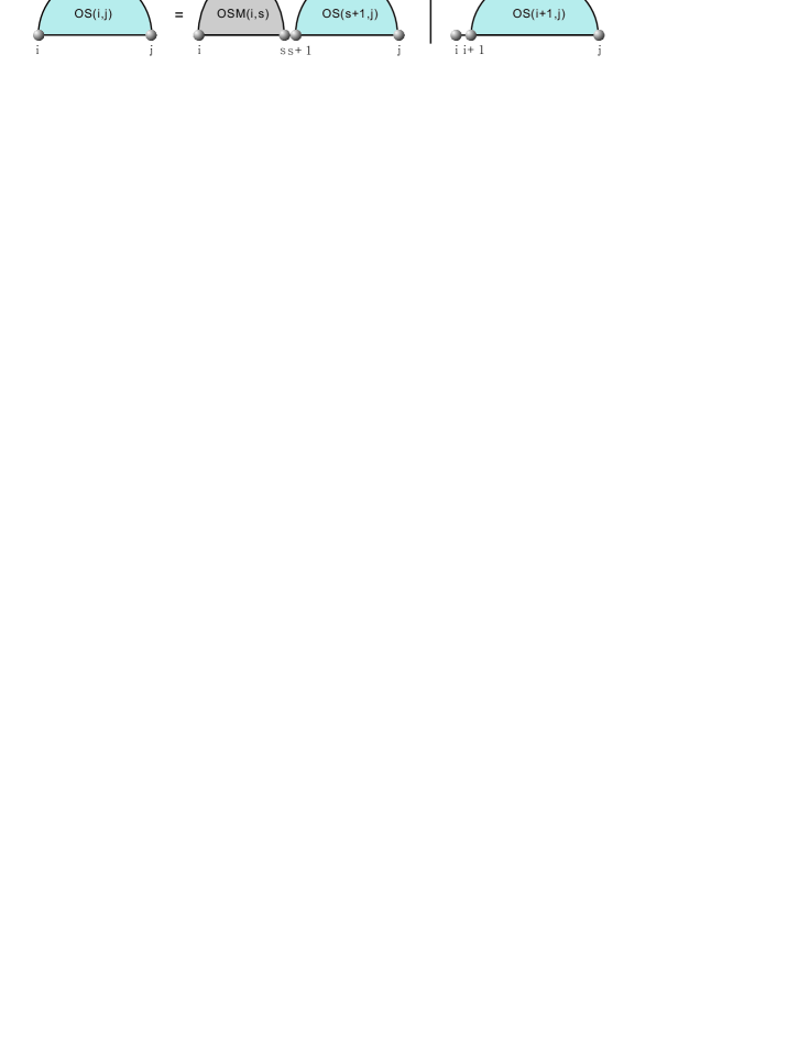
Figure 24. Constructing $OS(i,j)$: inductive decomposition of the optimal structure, $OS(i,j)$, into saturated skeleta, $OSM(i,s)$ and unpaired nucleotides.

Now we can inductively construct the array of structures $OS(i,j)$ and $OSM(i,j)$ via $OS$ and $OSM$ structures over smaller intervals. As a result, we finally obtain the structure $OS(1,n)$, i.e. the mfe-structure, see Fig.25.

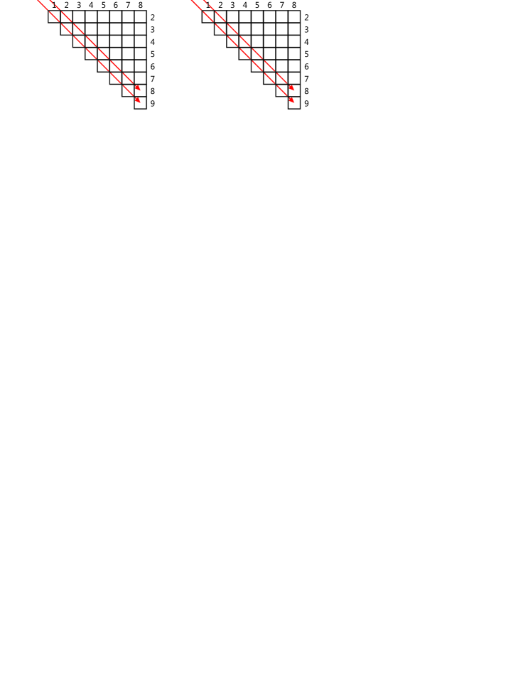
Figure 25. Inductive construction of $OS$ and $OSM$ structures: in the $s$-th step, we first construct $OSM(i,i+s)$, for any $0<i<n-s+1$. We then construct $OS(i,i+s)$ recruiting $OSM$-structures over intervals of lengths strictly smaller than $s$.

7. Synopsis

After providing the necessary background and context on pseudoknot folding routines and $k$-noncrossing structures, we discussed in detail in Sections 4,5 and 6 the three phases of cross, see Fig.26. Now, that the key ideas are presented, we proceed by integrating and discussing our results.

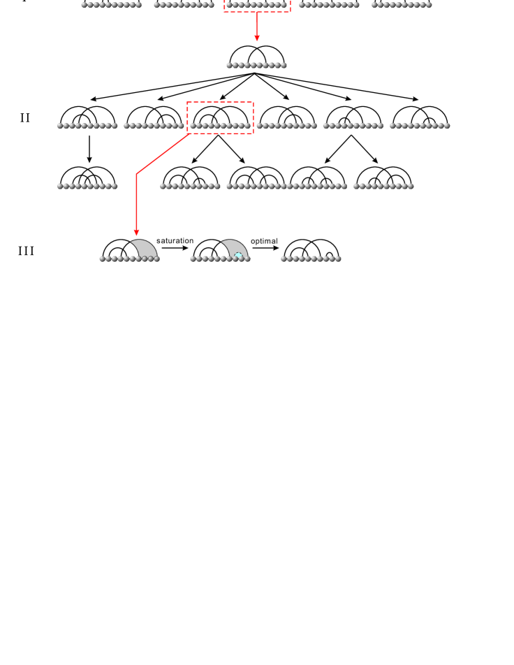
Figure 26. An outline of cross: the generation of motifs (I), the construction of skeleta-trees, rooted in irreducible shadows (II) and the saturation (III), during which, via DP-routines, optimal fillings of skeleta-intervals are derived.

Cross is an ab initio folding algorithms, which is guaranteed to search all $3$-noncrossing, $\sigma$-canonical structures and derives the corresponding loop-based mfe-configuration. A detailed description of the loop-energies as well as specific implementation particulars on how to generate the skeleta-trees of Section 5 via a certain matrix construction can be found at

$${\tt www.combinatorics.cn/cbpc/cross.html}$$

We remark that the code is improved and new features are being added, for instance, we currently work towards deriving the partition function version of cross, the generalization for arbitrary $k$ and a fully parallel implementation. The design of cross is fundamentally different from that of the pseudoknot DP-routines found in the literature. Point in case being the algorithm of [40], as outlined in Section 1. We showed that the latter cannot create any nonplanar $3$-noncrossing structure and furthermore cannot control the maximal number of mutually crossing arcs (crossing number). Consequently, DP-routines generate pseudoknot complexity by “just” increasing this very crossing number. The class of nonplanar $3$-noncrossing structures illustrates however, that structural complexity is not tantamount to the crossing number.

One key difference to any other pseudoknot folding algorithm is the fact that cross has a transparent, combinatorially specified, output class. This feature exists exclusively in secondary structure folding algorithms, where it is by construction implied. This specification is based on a novel combinatorial class, the $k$-noncrossing RNA structures and their exact and asymptotic enumeration [24, 25, 32]. The concept of $k$-noncrossing RNA structures is based on the combinatorial work of Chen et al. [6, 7]. The implications of this framework are profound: for $k=3,4,\dots,6$ it is possible, employing central limit theorems for $k$-noncrossing structures [26, 22] to derive a variety of generic properties of sequence-structure maps into RNA pseudoknot structures, irrespective of energy parameters [37, 21].

Furthermore cross is capable to generate novel classes of pseudoknots. Even in its current implementation, i.e. restriced to $3$-noncrossing structures it can generate any non-planar configuration. As mentioned already, the extension of cross to a version capable of folding any $k$-noncrossing structure, is work in progress. In this context, assertion (b) of Proposition 5.1 shows that novel constructions are required for efficient folding. Cross is by design an algorithm of exponential time complexity by virtue of its construction of its shadows and skeleta-trees. Only in its saturation phase it employs vector versions of DP-routines. Beyond the asymptotic analysis of motifs, given in Section 4, a detailed study of the performance of cross is work in progress. It appears however, that the folding times of random sequences are exponentially distributed. In Fig.27

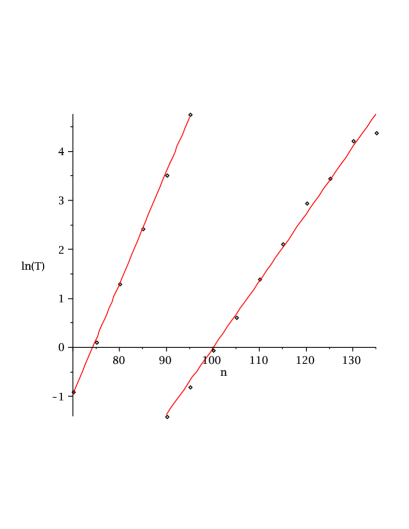
Figure 27. Mean folding times: we display the logarithm of the folding times of $1000$ random sequences as a function of the sequence length. For $3$-canonical and $4$-canonical structures the linear fits are given by $0.2263n-19.796$ (left) and $0.1364n-13.659$ (right), respectively.

we display the logarithm of the mean folding time of $1000$ random sequences. These data suggest exponential times with the exponential growth rates of $\approx 1.146$ and $\approx 1.254$, for $3$-canonical and $4$-canonical structures, respectively. In particular, a random sequence of length $100$ folded via a single core, $2.2$-GHz CPU exhibits a mean folding time of $279$ seconds with standard deviation of $267744$ seconds.

Acknowledgments. This work was supported by the 973 Project, the PCSIRT Project of the Ministry of Education, the Ministry of Science and Technology, and the National Science Foundation of China.

References

- [1] The HDV structure in nature. http://132.229.50.4/ batenburg/PKBase/PKB00075.html.
- [2] Mapping RNA form and function. Science, 2, 2005.
- [3] T. Akutsu. Dynamic programming algorithms for RNA secondary prediction with pseudoknots. Discr. Appl. Math., 104:45–62, 2000.
- [4] S. Cao and S. J. Chen. Predicting RNA pseudoknot folding thermodynamics. Nucl. Acids. Res., 34(9):2634–2652, 2006.
- [5] R. Cary and G. Stormo. Graph-theoretic approach to RNA modeling using comparative data. Proc. Int. Conf. Intell. Syst. Mol. Biol., 3:75–80, 1995.
- [6] W. Y. C. Chen, E. Y. P. Deng, R. R. X. Du, R. P. Stanley, and C. H. Yan. Crossings and nestings of matchings and partitions. Trans. Am. Math. Soc., 359:1555–1575, 2007.
- [7] W. Y. C. Chen, J. Qin, and C. M. Reidys. Crossing and nesting in tangled-diagrams. Elec. J. Comb., 15, 2008.
- [8] C. DeLisi and D. M. Crothers. Prediction of RNA secondary structure. Proc. Natl. Acad. Sci, USA, 68:2682–2685, 1971.
- [9] R. M. Dirks and N. A. Pierce. An algorithm for computing nucleic acid base-pairing probabilities including pseudoknots. J. Comput. Chem., 25:1295–1304, 2004.
- [10] S. R. Eddy. How do RNA folding algorithms work? Nature Biotechnology, 22:1457–1458, 2004.
- [11] J. Edmonds. Maximum matching and polyhedron with -vertices. J. Res. Nat. Bur. Stand., 69B:125–130, 1965.
- [12] J. R. Fresco, B. M. Alberts, and P. Doty. Some molecular details of the secondary structure of ribonucleic acid. Nature, 188:98–101, 1960.
- [13] H. N. Gabow. An efficient implementation of Edmonds’ algorithm for maximum matching on graphs. J. Asc. Com. Mach., 23:221–234, 1976.
- [14] I. Gessel and D. Zeilberger. Random walk in a weyl chamber. Proc. Amer. Math. Soc., 115:27–31, 1992.
- [15] W. Gruener, R. Giegerich, D. Strothmann, C. M. Reidys, Weber J., I. L. Hofacker, P. F. Stadler, and Schuster P. Analysis of RNA sequence structure maps by exhaustive enumeration i. neutral networks. Monatsh. Chem., 127:375–389, 1996.
- [16] W. Gruener, R. Giegerich, D. Strothmann, C. M. Reidys, Weber J., I. L. Hofacker, P. F. Stadler, and Schuster P. Analysis of RNA sequence structure maps by exhaustive enumeration. ii. Monatsh. Chem., 127:355–374, 1996.
- [17] I. L. Hofacker. Vienna RNA secondary structure server. Nucl. Acids. Res., 31(13):3429–3431, 2003.
- [18] I. L. Hofacker, M. Fekete, C. Flamm, M. A. Huynen, S. Rauscher, P. E. Stolorz, and P. F. Stadler. Automatic detection of conserved RNA structure elements in complete RNA virus genomes. Nucl. Acids. Res., 26:3825–2836, 1998.
- [19] I. L. Hofacker, W. Fontana, P. F. Stadler, L. S. Bonhoeffer, M. Tacker, and P. Schuster. Fast folding and comparison of RNA secondary structures. Monatsh. Chem., 125:167–188, 1994.
- [20] J. A. Howell, T. F. Smith, and M. S. Waterman. Computation of generating functions for biological molecules. J. Appl. Math., 39:119–133, 1980.
- [21] F. W. D. Huang, L. Y. M. Li, and C. M. Reidys. Sequence-structure relations of pseudoknot RNA. Bioinformatics. in press.
- [22] F. W. D. Huang and C. M. Reidys. Statistics of canonical RNA pseudoknot structures. J. Theor. Biol. in press.
- [23] M. Huynen, P. F. Stadler, and W. Fontana. Smoothness within ruggedness: the role of neutrality in adaptation. Proc. Natl. Acad. Sci, USA, 93:397–401, 1996.
- [24] E. Y. Jin, J. Qin, and C. M. Reidys. Combinatorics of RNA structures with pseudoknots. Bull. Math. Biol., 70(1):45–67, 2008.
- [25] E. Y. Jin and C. M. Reidys. RNA-lego: Combinatorial design of pseudoknot RNA. Adv. Appl. Math. in press.
- [26] E. Y. Jin and C. M. Reidys. Central and local limit theorems for RNA structures. J. Theor. Biol., 250(3):547–559, 2008.
- [27] E. Y. Jin, C. M. Reidys, and R. R. Wang. Asympotic enumeration of -noncrossing matchings. Submitted.
- [28] I. T. Jun, O. C. Uhlenbeck, and M. D. Levine. Estimation of secondary structure in ribonucleic acids. Nature, 230:362 – 367, 1971.
- [29] D. A. M. Konings and R. R. Gutell. A comparison of thermodynamic foldings with comparatively derived structures of 16s and 16s-like rRNAs. RNA, 1:559–574, 1995.
- [30] A. Loria and T. Pan. Domain structure of the ribozyme from eubacterial ribonuclease. RNA, 2:551–563, 1996.
- [31] R. B. Lyngsø and C. N. S. Pedersen. RNA pseudoknot prediction in energy-based models. J. Comput. Biol., 7:409–427, 2000.
- [32] G. Ma and C. M. Reidys. Canonical RNA pseudoknot structures. J. Comput. Biol. in press.
- [33] D. Metzler and M. E. Nebel. Predicting RNA secondary structures with pseudoknots by mcmc sampling. J. Math. Biol., 56(1-2):161–181, 2008.
- [34] R. Nussinov and A. B. Jacobson. Fast algorithm for predicting the secondary structure of single-stranded RNA. Proc. Natl. Acad. Sci, USA, 77:6309–6313, 1980.
- [35] J. Qin and C. M. Reidys. A combinatorial framework for RNA tertiary interaction. 2007. Submitted.
- [36] J. Reeder and Giegerich. R. Design, implementation and evaluation of a practical pseudoknot folding algorithm based on thermodynamics. Bioinformatics, 5(104), 2004.
- [37] C. M. Reidys. Local connectivity of neutral networks. Bull. Math. Biol.
- [38] P. F. Reidys, C. M. andStadler. Combinatorial landscapes. SIAM Review, 44:3–54, 2002.
- [39] J. Ren, B. Rastegari, A. Condon, and H. Hoos. Hotkonts: Heuristic prediction of RNA secondary structures including pseudoknots. RNA, 11:1494–1504, 2005.
- [40] E. Rivas and S. R. Eddy. A dynamic programming algorithm for RNA structure prediction including pseudoknots. J. Mol. Biol., 285(5):2053–2068, 1999.
- [41] E. Rivas and S. R. Eddy. The language of RNA: A formal grammar that includes pseudoknots. Bioinformatics, 16:326–333, 2000.
- [42] J. Ruan, G. Stormo, and W. Zhang. An iterated loop matching approch to the prediction. Bioinformatics, 20:58–66, 2004.
- [43] P. Schuster and W. Fontana. Chance and necessity in evolution: Lessons from RNA. Physica. D., 133:427–452, 1999.
- [44] P. Schuster, W. Fontana, P. F. Stadler, and I. L. Hofacker. From sequences to shapes and back: A case study in RNA secondary structures. Proc. Roy. Soc. Lond. B, 255:279–284, 1994.
- [45] D. B. Searls. The language of genes. Nature, 420:211–217, 2002.
- [46] T. F. Smith and M. S. Waterman. RNA secondary structure. Math. Biol., 42:31–49, 1978.
- [47] J. Tabaska, R. Cary, H. Gabow, and G. Stormo. An RNA folding method capable of identifying pseudoknots and base triples. Bioinformatics, 14:691–699, 1998.
- [48] M. Tacker, P. F. Stadler, E. G. Bornberg-Bauer, Schuster P., I. L. Hofacker, and P. Schuster. Algorithm independent properties of RNA secondary structure predictions. Europ. Biophy. J., 25:115–130, 1996.
- [49] I. Tinoco, P. N. Borer, B. Dengler, M. D. Levine, O. C. Uhlenbeck, D. M. Crothers, and J. Gralla. Improved estimation of secondary structure in ribonucleic acids. Nature New Biology, 246:40–41, 1973.
- [50] Y. Uemura, A. Hasegawa, S. Kobayashi, and T. Yokomori. Tree adjoining grammars for RNA structure prediction. Theor. Comput. Sci., 210:277–303, 1999.
- [51] M. S. Waterman. Combinatorics of RNA hairpins and cloverleaves. Stud. Appl. Math., 60:91–96, 1979.
- [52] M. S. Waterman and T. F. Smith. Rapid dynamic programming methods for RNA secondary structure. Adv. Appl. Math., 7:455–464, 1986.
- [53] E. Westhof and L. Jaeger. RNA pseudoknots. Curr. Opin. Struct. Biol., 2:327–333, 1992.
- [54] M. Zuker and P. Stiegler. Optimal computer folding of large RNA sequences using thermodynamics and auxiliary information. Nucl. Acids. Res., 9:133–148, 1981.