Estimation of Higher Order Moments for Compound Models of Clutter by Mellin Transform

Abstract

The compound models of clutter statistics are found suitable to describe the nonstationary nature of radar backscattering from high-resolution observations. In this letter, we show that the properties of Mellin transform can be utilized to generate higher order moments of simple and compound models of clutter statistics in a compact manner.

I Introduction

Radar backscattering from ground or sea surfaces are wide-sense stationary for low-resolution observations as expectations of clutter statistics or moments are assumed to be independent of spatio-temporal changes. For high-resolution observations, such surfaces reveal heterogeneous structures such as swell in sea waves or winds blowing over the canopy of grasslands that result in nonstationary clutter statistics [1], [2], [4]. The compound models of probability density functions (pdf) incorporate the variation in the parameters of clutter in such cases.

Traditionally higher order moments of a continuous random variable (rv) X are generated from higher order derivatives of its characteristic function defined as

$$\Phi_{\emph{{X}}}(\omega)=\emph{E}\{\exp(\emph{j}\omega\emph{x})\}=\int_{-\infty}^{\infty}\emph{f}_{\textbf{\emph{X}}}(\emph{x})\exp(\emph{j}\omega\emph{x})\emph{dx}\textrm{.}$$ (1)

The continuous pdf $\emph{f}_{\textbf{\emph{X}}}(\emph{x})$ is for $-\infty<\emph{x}<\infty$. Generation of moments and cumulants from (1) for the compound models of clutter require solutions of incomplete integrals. The domain of X is $0\leq\emph{x}<\infty$ for amplitude and power statistics, and $\int_{0}^{\infty}\emph{f}_{\textbf{\emph{X}}}(\emph{x})\emph{dx}=1$. Properties of Mellin transform provide the formalism to derive higher order moments in a compact manner in such cases. Some of these properties were used in [3], [6] to derive the moments for high-resolution synthetic aperture radar (SAR) clutter statistics. Here, we show that the properties of Mellin transform can be utilized in an effective manner for both simple and compound models of clutter either in amplitude or in intensity domain.

II Mellin Transform Properties

Mellin transform exists for a continuous function $\emph{f}_{\textbf{\emph{X}}}(\emph{x})$ defined over $\mathbb{R}_{+}$. The transform operator is the second kind characteristic function $\Phi_{\emph{{X}}}(s)$ expressed as

$$\Phi_{\emph{{X}}}(s)=\mathcal{M}[\emph{f}_{\textbf{\emph{X}}}(\emph{x});\emph{s}]=\int_{0}^{\infty}\emph{x}^{\emph{s}-1}\emph{f}_{\textbf{\emph{X}}}(\emph{x})\emph{dx}\textrm{.}$$ (2)

Here $\emph{s}=\emph{a}+\emph{j}\emph{b}\in\mathbb{C}$ is the complex Laplace transform variable. Traditional moments are generated from (2) with $\emph{s}=\emph{n}+1,\emph{n}\in\mathbb{Z}_{+}.$

$$\emph{m}_{\emph{n}}=\mathcal{M}{\displaystyle\biggl{[}\emph{f}_{\textbf{\emph{X}}}(\emph{x});\emph{s}\biggr{]}}_{\emph{s}=\emph{n}+1}\textrm{.}$$ (3)

Second-kind moments or the log-moments are generated for logarithm of rv X by using the derivative property of Mellin transform.

$$\tilde{\emph{m}_{\emph{n}}}=\mathcal{M}[\log(\emph{x})^{\emph{n}}\emph{f}_{\textbf{\emph{X}}}(\emph{x});\emph{s}]\bigg{|}_{\emph{s}=1}=\int_{0}^{\infty}\emph{x}^{\emph{s}-1}\log(\emph{x})^{\emph{n}}\emph{f}_{\textbf{\emph{X}}}(\emph{x})\emph{dx}$$

$$\qquad=\frac{d^{\emph{n}}}{d\emph{s}^{\emph{n}}}\Phi_{\emph{{X}}}(\emph{s})\bigg{|}_{\emph{s}=1}\textrm{.}\qquad\qquad$$ (4)

Analogous to the cumulants derived from logarithm of characteristic function in (1), the n-th order cumulants of second kind or the log-cumulants are obtained from derivatives of logarithm of $\Phi_{\emph{{X}}}(s)$; i.e., $\Psi_{\emph{{X}}}(s)=\log(\Phi_{\emph{{X}}}(s))$.

$$\tilde{\emph{k}_{\emph{n}}}=\frac{d^{\emph{n}}}{d\emph{s}^{\emph{n}}}\Psi_{\emph{{X}}}(\emph{s})\bigg{|}_{\emph{s}=1}\textrm{.}$$ (5)

The log-moments and the log-cumulants are related as

$$\tilde{\emph{k}_{1}}=\tilde{\emph{m}_{1}}$$

$$\tilde{\emph{k}_{2}}=\tilde{\emph{m}_{2}}-\tilde{\emph{m}_{1}}^{2}$$

$$\tilde{\emph{k}_{3}}=\tilde{\emph{m}_{3}}-3\tilde{\emph{m}_{1}}\tilde{\emph{m}_{2}}+2\tilde{\emph{m}_{1}}^{3}$$

$$\tilde{\emph{k}_{4}}=\tilde{\emph{m}}_{4}-4\tilde{\emph{m}_{1}}\tilde{\emph{m}_{3}}+6\tilde{\emph{m}_{1}}^{2}\tilde{\emph{m}_{2}}-3\tilde{\emph{m}_{1}}^{4}\textrm{.}$$ (6)

The underlying mean of speckle component of clutter vary widely in the compound models of amplitude or power statistics resulting in long-tailed distributions. Speckle arises from randomness in the distribution of backscattering elements in the resolution cell, the number of such scatterers is nonstationary for high-resolution observations. The pdf of high-resolution clutter is described by taking into account of a rv Z signifying randomness in the mean of clutter.

$$\qquad\emph{f}_{\textbf{\emph{X}}}(\emph{x})=\int_{0}^{\infty}\emph{f}_{\textbf{\emph{X}}}(\emph{x}|\emph{z})\emph{f}_{\textbf{\emph{Z}}}(\emph{z})\emph{dz}{}{},\qquad\emph{z}>0\textrm{.}$$ (7)

The compound pdf model in (7) is a Mellin convolution. One nice property of Mellin transform is the product form of the components of pdf in the transform domain [5].

$$\mathcal{M}[\emph{f}_{\textbf{\emph{X}}}(\emph{x});\emph{s}]=\mathcal{M}[\emph{f}_{\textbf{\emph{X}}}(\emph{x}|\emph{z});\emph{s}]\mathcal{M}[\emph{f}_{\textbf{\emph{Z}}}(\emph{z});\emph{s}]\textrm{.}$$ (8)

The log-cumulants of the components in (8) are therefore additive.

$$\tilde{\emph{k}_{\emph{n},\emph{x}}}=\tilde{\emph{k}_{\emph{n},(\emph{x},\emph{z})}}+\tilde{\emph{k}_{\emph{n},\emph{z}}}\textrm{.}$$ (9)

III Moments Generation for Simple Models of Clutter

The shape and scale parameters of simple models of pdf for low-resolution cases are stationary. The usual pdf of speckle power is a gamma distribution resulting from convolution of L independent exponential distributions.

$$\emph{f}_{\textbf{\emph{V}}}(\emph{v})=\frac{1}{\Gamma(\emph{L})}{\bigg{(}\frac{\emph{L}}{\mu}\bigg{)}}^{\emph{L}}\emph{v}^{(\emph{L}-1)}\exp\bigg{(}-\frac{\emph{L}\emph{v}}{\mu}\bigg{)},\qquad\emph{v}\geq 0\textrm{.}$$ (10)

Here $\Gamma(.)$ is the standard gamma function. The shape and scale of distribution are determined by L and $\mu$, mean value of clutter power respectively. Corresponding amplitude distribution turns out to be a Nakagami pdf [2], [6].

$$\emph{f}_{\textbf{\emph{N}}}(\emph{r})=\frac{2}{\Gamma(\emph{L})}\bigg{(}\frac{{\sqrt{\emph{L}}}}{\mu}\bigg{)}^{2\emph{L}}\emph{r}^{(2\emph{L}-1)}\exp\bigg{(}-\frac{\emph{L}\emph{r}^{2}}{\mu^{2}}\bigg{)},\quad\emph{r}\geq 0\textrm{.}$$ (11)

Mellin transform for gamma pdf is

$$\Phi_{\emph{{G}}}(\emph{s})=\frac{\lambda^{\emph{L}}}{\Gamma(\emph{L})}\int_{0}^{\infty}\emph{v}^{(\emph{L+s}-1)-1}\exp(-\lambda\emph{v})\emph{dv}$$ (12)

with $\lambda=\frac{\emph{L}}{\mu}$. Using the transform pair

$$\mathcal{M}[\emph{x}^{\emph{u}}\exp(-\lambda\emph{x});\emph{s}]\Longleftrightarrow\lambda^{-(\emph{s}+\emph{u})}\Gamma(\emph{s}+\emph{u})$$

we obtain,

$$\Phi_{\emph{{G}}}(\emph{s})=\bigg{(}\frac{\mu}{\emph{L}}\bigg{)}^{\emph{s}-1}\frac{\Gamma(\emph{s}+\emph{L}-1)}{\Gamma(\emph{L})}\textrm{.}$$ (13)

The moments of first kind for gamma pdf are generated from (13) with $\emph{s}=\emph{n}+1$ as

$$\emph{m}_{\emph{n}}=\Phi_{\emph{{G}}}(\emph{s})\bigg{|}_{\emph{s}=\emph{n}+1}=\bigg{(}\frac{\mu}{\emph{L}}\bigg{)}^{\emph{n}}\frac{\Gamma(\emph{L}+\emph{n})}{\Gamma(\emph{L})}\textrm{.}$$ (14)

As a special case of the result in (14), the moments of exponential pdf (for $\emph{L}=1$) are $\emph{m}_{\emph{n}}=\mu^{\emph{n}}{\emph{n}}!$. Maxwell pdf is the case for $\emph{L}=3$.

$$\emph{f}_{\textbf{\emph{M}}}(\emph{u})=\frac{1}{\sigma^{3}}\sqrt{\frac{2}{\pi}}\emph{u}^{2}\exp\bigg{(}-\frac{\emph{u}^{2}}{2\sigma^{2}}\bigg{)},\qquad\emph{u}\geq 0\textrm{.}$$ (15)

We use the additional Mellin transform pair

$$\mathcal{M}[\exp(-\lambda\emph{x}^{2});\emph{s}]\Longleftrightarrow\frac{1}{2}(\lambda)^{-\frac{s}{2}}\Gamma(\frac{\emph{s}}{2})$$

with $\lambda=\frac{1}{2\sigma^{2}}$ ; so that

$$\Phi_{\emph{{M}}}(\emph{s})=\frac{1}{\sigma}\sqrt{\frac{2}{\pi}}(2\sigma^{2})^{\frac{\emph{s}}{2}}{\frac{\emph{s}}{2}}\Gamma\bigg{(}\frac{\emph{s}}{2}\bigg{)}\textrm{.}$$ (16)

The moments of first kind for Maxwell pdf are

$$\emph{m}_{\emph{n}}=\Phi_{\emph{{M}}}(\emph{s})\bigg{|}_{\emph{s}=\emph{n}+1}=\frac{1}{\sigma}\sqrt{\frac{2}{\pi}}(2\sigma^{2})^{\frac{\emph{n}+1}{2}}\bigg{(}\frac{\emph{n}+1}{2}\bigg{)}\Gamma\bigg{(}\frac{\emph{n}+1}{2}\bigg{)}\textrm{.}$$ (17)

The moments for amplitude distributions are also derived by Mellin transform. As for Nakagami distribution, with $\lambda=\frac{\sqrt{\emph{L}}}{\mu}$

$$\Phi_{\emph{{N}}}(\emph{s})=\frac{2}{\Gamma(\emph{L})}(\lambda^{2})^{\emph{L}}\int_{0}^{\infty}\emph{r}^{(\emph{s}+2\emph{L}-1)-1}\exp(-\lambda^{2}\emph{r}^{2})\emph{dr}$$

$$\qquad\qquad=\bigg{(}\frac{\sqrt{\emph{L}}}{\mu}\bigg{)}^{-(\emph{s}-1)}\frac{\Gamma(\emph{L}+\frac{\emph{s}-1}{2})}{\Gamma(\emph{L})}\textrm{.}\qquad\qquad\qquad$$ (18)

The log-cumulants are easier to derive here. In general the log-cumulants of Nakagami distribution are derived from (5)

$$\tilde{\emph{k}_{\emph{n}}}=\bigg{(}\frac{1}{2}\bigg{)}^{\emph{n}}\mathbf{\Upsilon}(\emph{n}-1,\emph{L})\textrm{.}$$ (19)

Here $\mathbf{\Upsilon}(.)$ is the Digamma function; i. e., the first derivative of $\ln\Gamma(\emph{s})$ at $\emph{s}=1$. In general $\mathbf{\Upsilon}(\emph{n}-1,\emph{L})$ is the nth derivative of the Digamma function for variable L.

One long-tailed pdf often used in sea-clutter amplitude modelling [1] is Weibull distribution.

$$\emph{f}_{\textbf{\emph{W}}}(\emph{x};\emph{z},\emph{b})=\bigg{(}\frac{\emph{b}}{\emph{z}}\bigg{)}\bigg{(}\frac{\emph{x}}{\emph{z}}\bigg{)}^{\emph{b}-1}\exp{\displaystyle\bigl{[}-\bigg{(}\frac{\emph{x}}{\emph{z}}\bigg{)}^{b}\bigr{]}},{}{}\emph{x}\geq 0;\emph{b},\emph{z}>0\textrm{.}$$ (20)

Here z is the scale parameter and b is the shape parameter of distribution. Mellin transform of (20) is

$$\Phi_{\emph{{W}}}(\emph{s})=\frac{\emph{b}}{\emph{z}^{\emph{b}}}\int_{0}^{\infty}\emph{x}^{(\emph{s}+\emph{b}-1)-1}\exp{\displaystyle\bigl{[}-\bigg{(}\frac{\emph{x}}{\emph{z}}\bigg{)}^{b}\bigr{]}}\emph{dx}\textrm{.}$$ (21)

From the Mellin transform pair

$$\mathcal{M}[{\exp(-\lambda\emph{x}^{\emph{b}})};\emph{s}]\Longleftrightarrow\emph{b}^{-1}\lambda^{-\frac{\emph{s}}{\emph{b}}}\Gamma(\frac{\emph{s}}{\emph{b}}),$$

the second characteristic function is

$$\Phi_{\emph{{W}}}(\emph{s})=\emph{z}^{(\emph{s}-1)}\Gamma\big{(}\frac{\emph{s}+\emph{b}-1}{\emph{b}}\big{)}\textrm{.}$$ (22)

The moments of first kind for Weibull distribution are

$$\emph{m}_{\emph{n}}=\Phi_{\emph{{W}}}(\emph{s})\bigg{|}_{\emph{s}=\emph{n}+1}=\emph{z}^{\emph{n}}\Gamma\big{(}\frac{\emph{n}+\emph{b}}{\emph{b}}\big{)}\textrm{.}$$ (23)

The common Rayleigh amplitude pdf is a special case of Weibull distribution with $b=2$.

$$\emph{f}_{\textbf{\emph{R}}}(\emph{r};\emph{z})=2\bigg{(}\frac{\emph{r}}{\emph{z}^{2}}\bigg{)}\exp{\displaystyle\bigl{[}-\bigg{(}\frac{\emph{r}}{\emph{z}}\bigg{)}^{2}\bigr{]}},\qquad\emph{r}\geq 0\textrm{.}$$ (24)

The moments of first kind for Rayleigh pdf are

$$\emph{m}_{\emph{n}}=\Phi_{\emph{{R}}}(\emph{s})\bigg{|}_{\emph{s}=\emph{n}+1}=\emph{z}^{\emph{n}}\Gamma\bigg{(}\frac{\emph{n}+2}{2}\bigg{)}\textrm{.}$$ (25)

We show in the next section the utility of Mellin transform for deriving the log-moments and the log-cumulants of compound models of clutter in a compact manner.

IV Moments Generation for Compound Models of Clutter

The pdf for compound models of high-resolution clutter have got two components; pdf of speckle component, and pdf of the modulation in mean amplitude or power of speckle. Considering both to be gamma distributed rv the pdf for generalized gamma (G$\Gamma$) model of clutter power is [6]

$$\emph{f}_{\textbf{\emph{V}}}(\emph{v})=\frac{1}{\Gamma(\emph{L})\Gamma(\emph{M})}\bigg{(}\frac{2\emph{L}\emph{M}}{<\emph{z}>}\bigg{)}\bigg{(}\frac{2\emph{L}\emph{M}}{<\emph{z}>}\emph{v}\bigg{)}^{(\frac{\emph{L}+\emph{M}-2}{2})}$$

$$\qquad\qquad\qquad\emph{K}_{{\emph{M}}-{\emph{L}}}{\displaystyle\bigl{[}2\bigg{(}\frac{\emph{LM}}{<\emph{z}>}\emph{v}\bigg{)}^{\frac{1}{2}}\bigr{]}}\textrm{.}$$ (26)

The shape parameter for gamma pdf $\emph{f}_{\textbf{\emph{Z}}}(\emph{z})$ of rv Z according to (7) is M, and $\emph{K}_{\emph{M}-\emph{L}}(.)$ is the second kind modified Bessel function of order $(\emph{M}-\emph{L})$. The mean estimate of $<\emph{z}>=\mu$. Assuming speckle and the modulation in mean power in the high-resolution cell to be independent of each other, we have by Mellin convolution property in (8)

$$\Psi_{\emph{{V}}}(s)=(\emph{s}-1)\log\bigg{(}\frac{\mu}{\emph{LM}}\bigg{)}+\log\Gamma(\emph{s}+\emph{L}-1)+$$

$$\qquad\qquad{}{}\log\Gamma(\emph{s}+\emph{M}-1)-\log\Gamma(\emph{L})-\log\Gamma(\emph{M})\textrm{.}$$ (27)

The log-cumulants of G$\Gamma$ model are

$${}\tilde{\emph{k}_{1}}=\log\bigg{(}\frac{\mu}{\emph{LM}}\bigg{)}+\mathbf{\Upsilon}(\emph{L})+\mathbf{\Upsilon}(\emph{M})\bigg{|}_{\emph{s}=1}$$

$${}\tilde{\emph{k}_{\emph{n}}}=\mathbf{\Upsilon}(\emph{n}-1,\emph{L})+\mathbf{\Upsilon}(\emph{n}-1,\emph{M})\textrm{.}$$ (28)

Spikes in high-resolution ground-clutter amplitude at low grazing angles are often described by the K-distribution model [2], [4]. The compound K-pdf

$$\emph{f}_{\textbf{\emph{N}}}(\emph{r})=\frac{4\emph{b}^{\frac{(\alpha+1)}{2}}\emph{r}^{\alpha}}{\Gamma(\alpha)}\emph{K}_{{\alpha}-1}(2\emph{r}\sqrt{\emph{b}})$$ (29)

is a Mellin convolution of Rayleigh pdf and exponential pdf given by,

$$\emph{f}_{\textbf{\emph{N}}}(\emph{r})=\frac{4\emph{r}\emph{b}^{\alpha}}{\Gamma(\alpha)}\int_{0}^{\infty}\frac{\emph{dz}}{\emph{z}}\emph{z}^{\alpha-1}\exp\bigg{(}-\emph{b}\emph{z}-\frac{\emph{r}^{2}}{\emph{z}}\bigg{)}\textrm{.}$$ (30)

Here $\alpha$ is the shape parameter in the variation of mean of sea or ground clutter amplitude, and b is the scale parameter for associated speckle amplitude. Following derivation for Nakagami pdf in (19) the second characteristics function for K-pdf is given by,

$$\Phi_{\emph{{N}}}(\emph{s})=\emph{b}^{-(\frac{\emph{s}-1}{2})}\mu^{\emph{s}-1}\Gamma\bigg{(}\frac{\emph{s}}{2}+\frac{1}{2}\bigg{)}\frac{\Gamma(\alpha+\frac{\emph{s}-1}{2})}{\Gamma(\alpha)}\textrm{ .}$$ (31)

where $<\emph{z}>=\mu^{2}$. The log-cumulants for K-pdf are

$$\Psi_{\emph{{N}}}(s)=-\bigg{(}\frac{\emph{s}-1}{2}\bigg{)}\log\emph{b}+(\emph{s}-1)\log\mu+\log\Gamma\bigg{(}\frac{\emph{s}}{2}+\frac{1}{2}\bigg{)}+$$

$$\qquad\log\Gamma\bigg{(}\alpha+\frac{\emph{s}-1}{2}\bigg{)}-\log\Gamma(\alpha),$$

and

$${}\tilde{\emph{k}_{1}}=-\frac{1}{2}\log\emph{b}+\log\mu+\frac{1}{2}\mathbf{\Upsilon}(\alpha)+\frac{1}{2}\mathbf{\Upsilon}(1)\bigg{|}_{\emph{s}=1}$$

$${}\tilde{\emph{k}_{\emph{n}}}=\bigg{(}\frac{1}{2}\bigg{)}^{\emph{n}}\mathbf{\Upsilon}(\emph{n}-1,\alpha)\textrm{.}$$ (32)

Here $\mathbf{\Upsilon}(1)=-0.577215$ is the Euler constant [5]. This shows that the log-cumulants of K-distribution are determined by the higher order log-cumulants of Nakagami distribution in the mean of high-resolution ground or sea clutter.

A more extended case of compound clutter model is the scene where variation in the shape of clutter amplitude distribution is given by generalized Weibull distribution [4].

$$\emph{f}_{\textbf{\emph{WN}}}(\emph{r};\emph{b},\emph{c},\alpha)=\frac{2\emph{c}\emph{b}^{\alpha}}{\Gamma(\alpha)}\emph{r}^{\emph{c}-1}\int_{0}^{\infty}\frac{\emph{dz}}{\emph{z}^{\emph{c}}}\emph{z}^{2\alpha-1}\exp\bigg{[}-\bigg{(}\frac{\emph{r}}{\emph{z}}\bigg{)}^{\emph{c}}-\emph{b}\emph{z}^{2}\bigg{]}\textrm{.}$$ (33)

This is a Mellin convolution where randomness in the mean amplitude of clutter is described by Nakagami pdf with the shape parameter being $\alpha$.

$$\emph{f}_{\textbf{\emph{N}}}(\emph{z};\emph{b},\alpha)=\frac{2\emph{b}^{\alpha}}{\Gamma(\alpha)}\emph{z}^{2\alpha-1}\exp({-\emph{b}\emph{z}^{2}}),$$

and the clutter amplitude follows a generalized Weibull distribution with the shape parameter being c.

$$\emph{f}_{\textbf{\emph{W}}}(\emph{r}|\emph{z};\emph{c})=\frac{\emph{c}}{\emph{z}^{\emph{c}}}\emph{r}^{\emph{c}-1}\exp\bigg{[}-\bigg{(}\frac{\emph{r}}{\emph{z}}\bigg{)}^{\emph{c}}\bigg{]}\textrm{.}$$

Following the transform rule of Mellin convolution,

$${}\Phi_{\emph{{W}{N}}}(\emph{s})=\Phi_{\emph{{W}}}(\emph{s})\Phi_{\emph{{N}}}(\emph{s})\qquad$$

$${}\qquad=\bigg{(}\frac{\sigma}{\emph{b}}\bigg{)}^{\frac{\emph{s}-1}{2}}\Gamma\bigg{(}\frac{\emph{s}+\emph{c}-1}{c}\bigg{)}\frac{\Gamma\big{(}\alpha+\frac{\emph{s}-1}{2}\big{)}}{\Gamma(\alpha)}\textrm{.}$$ (34)

where $<\emph{z}^{2}>=\sigma$. The log-moments for this generalized Weibull model of clutter according to (9) are

$${}\tilde{\emph{k}_{1}}=\frac{1}{2}\log\bigg{(}\frac{\sigma}{\emph{b}}\bigg{)}+\frac{1}{\emph{c}}\mathbf{\Upsilon}(1)+\frac{1}{2}\mathbf{\Upsilon}(\alpha)\bigg{|}_{\emph{s}=1}$$

$${}\tilde{\emph{k}_{\emph{n}}}=\bigg{(}\frac{1}{2}\bigg{)}^{\emph{n}}\mathbf{\Upsilon}(\emph{n}-1,\alpha)\textrm{.}$$ (35)

Another compound model used to describe high-resolution SAR clutter is the Fisher distribution [3].

$$\emph{f}_{\textbf{\emph{F}}}(\emph{u})=\frac{\Gamma(\emph{L}+\emph{M})}{\Gamma(\emph{L})\Gamma(\emph{M})}\bigg{(}\frac{\emph{L}}{\emph{M}\mu}\bigg{)}\frac{\big{(}\frac{\emph{L}}{\emph{M}\mu}\emph{u}\big{)}^{\emph{L}-1}}{\big{(}1+\frac{\emph{L}}{\emph{M}\mu}\emph{u}\big{)}^{\emph{L}+\emph{M}}}\textrm{.}$$ (36)

Consider $\frac{\emph{L}}{\emph{M}\mu}\emph{u}=\lambda$; following the Mellin transform pair

$$\mathcal{M}[(1+\lambda)^{-\emph{b}};\emph{s}]\Longleftrightarrow\frac{\Gamma(\emph{s})\Gamma(\emph{b}-\emph{s})}{\Gamma(\emph{b})},\textrm{ with }\emph{b}=\emph{L}+\emph{M}$$

the second characteristic function for Fisher distribution is

$$\Phi_{\emph{{F}}}(\emph{s})=\bigg{(}\frac{\emph{M}\mu}{\emph{L}}\bigg{)}^{\emph{s}-1}\frac{1}{\Gamma(\emph{L})(\emph{M})}\Gamma(\emph{s}+\emph{L}-1)\Gamma(\emph{M}+1-\emph{s})\textrm{.}$$ (37)

Corresponding log-cumulants are

$${}\tilde{\emph{k}_{1}}=\log\mu+[\mathbf{\Upsilon}(\emph{L})-\log\emph{L}]+[\mathbf{\Upsilon}(\emph{M})-\log\emph{M}]\bigg{|}_{\emph{s}=1}$$

$${}\tilde{\emph{k}_{\emph{n}}}=\mathbf{\Upsilon}(\emph{n}-1,\emph{L})+(-1)^{\emph{n}}\mathbf{\Upsilon}(\emph{n}-1,\emph{M})\textrm{.}$$ (38)

One useful application of the log-cumulants and their relationship with the log-moments in (II) is estimation of parameters of texture. Empirical data from high-resolution radar backscattering $\emph{x}(\emph{t})$ follow the product model,

$$\emph{x}(\emph{t})=\emph{u}(\emph{t})\emph{z}(\emph{t})\textrm{.}$$ (39)

Here $\emph{u}(\emph{t})$ is the speckle component, and $\emph{z}(\emph{t})$ represent texture signifying variation in the mean parameter. The log-moments of observed data and the log-cumulants of texture can be estimated for different compound models utilizing the relationships in (II) and (II). Parameters for texture are derived using the log-cumulants of speckle as in (9), and can be verified with the theoretical values derived in the paper. For example, second and fourth order log-cumulants of texture component for G$\Gamma$ model of high-resolution ground clutter in (IV) are estimated in Fig. 1. Second and fourth order log-moments of $\emph{x}(\emph{t})$ are derived from the log-cumulants of $\emph{z}(\emph{t})$ assuming it to be a gamma variable, and $\emph{u}(\emph{t})$ also follows gamma distribution. The results of simulation show that higher order log-cumulants of texture vanish with increasing values of shape parameter M. This is expected in the present case as the texture component follows a nearly Gaussian distribution with constant mean for increasing values of M. For values of $\emph{M}<1$, there is presence of large amount of spikes in observed data signifying high values of log-moments and cumulants. Log-moments of clutter tend to become constant with increasing M signifying stationarity of low-resolution observations.

V Conclusion

The utility of Mellin transform properties to generate higher order moments of simple and compound models of clutter in both amplitude and power domain is shown in this letter. The second kind characteristic function and its properties provide compact analytical expressions for higher order moments that are useful to interpret texture properties of high-resolution clutter.

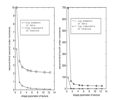
Figure 1: Log-moments of data and log-cumulants of texture for simulation of G$\Gamma$ model of high-resolution clutter. Left: second order moments; right: fourth order moments.

References

• [1] F. L.  Posner, ”Spiky sea clutter at high range resolutions and very low grazing angles,” IEEE Trans. Aerospace and Electronic Systems, vol. 38, no.1, pp. 58-73, Jan 2002.
• [2] M. S.  Greco, and F.  Gini, ”Statistical analysis of high-resolution SAR ground clutter data,” IEEE Trans. Geoscience and Remote Sensing, vol. 45, no. 3, pp. 566-575, March 2007.
• [3] C.  Tison, J. -M.  Nicolas, F.  Tupin, and H.  Maitre, ”A new statistical model for Markovian classification of urban areas in high-resolution SAR images,” IEEE Trans. Geoscience and Remote Sensing, vol. 42, no. 10, pp. 2046-2057, October 2004.
• [4] V.  Anastassopoulos, G. A.  Lampropoulos, A.  Drosopoulos, and M.  Rey, ”High resolution radar clutter statistics,” IEEE Trans. Aerospace and Electronic Systems, vol. 35, no. 1, pp. 43-60, Jan. 1999.
• [5] A. D. Poularikas, The Handbook of Formulas and Tables for Sigmal Processing, Florida, USA: CRC and IEEE Press, 1999.
• [6] G.  Moser, J.  Zerubia, and S. B.  Serpico, ”SAR amplitude probability density function estimation based on a generalized Gaussian model,” IEEE Trans. Image Processing, vol. 15, no. 6, pp. 1429-1442, June 2006.