Hypercompact Stellar Systems Around Recoiling Supermassive Black Holes

Abstract

A supermassive black hole ejected from the center of a galaxy by gravitational wave recoil carries a retinue of bound stars – a “hypercompact stellar system” (HCSS). The numbers and properties of HCSSs contain information about the merger histories of galaxies, the late evolution of binary black holes, and the distribution of gravitational-wave kicks. We relate the structural properties (size, mass, density profile) of HCSSs to the properties of their host galaxies and to the size of the kick, in two regimes: collisional ($M_{\rm BH}\;\hbox to0.0pt{\lower 2.5pt\hbox{$\sim$}\hss}\raise 1.5pt\hbox{$<$}\;10^{7}M_{\odot}$), i.e. short nuclear relaxation times; and collisionless ($M_{\rm BH}\;\hbox to0.0pt{\lower 2.5pt\hbox{$\sim$}\hss}\raise 1.5pt\hbox{$>$}\;10^{7}M_{\odot}$), i.e. long nuclear relaxtion times. HCSSs are expected to be similar in size and luminosity to globular clusters but in extreme cases (large galaxies, kicks just above escape velocity) their stellar mass can approach that of ultra-compact dwarf galaxies. However they differ from all other classes of compact stellar system in having very high internal velocities. We show that the kick velocity is encoded in the velocity dispersion of the bound stars. Given a large enough sample of HCSSs, the distribution of gravitational-wave kicks can therefore be empirically determined. We combine a hierarchical merger algorithm with stellar population models to compute the rate of production of HCSSs over time and the probability of observing HCSSs in the local universe as a function of their apparent magnitude, color, size and velocity dispersion, under two different assumptions about the star formation history prior to the kick. We predict that $\sim 10^{2}$ HCSSs should be detectable within 2 Mpc of the center of the Virgo cluster and that many of these should be bright enough that their kick velocities (i.e. velocity dispersions) could be measured with reasonable exposure times. We discuss other strategies for detecting HCSSs and speculate on some exotic manifestations.

1. Introduction

A natural place to search for supermassive black holes (SMBHs) is at the centers of galaxies, where they presumably are born and spend most of their lives. But it has become increasingly clear that a SMBH can be violently separated from its birthplace as a result of linear momentum imparted by gravitational waves during strong-field interactions with other SMBHs (Peres, 1962; Bekenstein, 1973; Redmount & Rees, 1989). The largest net recoils are produced from configurations that bring the two holes close enough together to coalesce. Kick velocities following coalescence can be as high as $\sim 200$ km s^-1 in the case of nonspinning holes (González et al. 2007a, ; Sopuerta et al., 2007); $\sim 4000$ km s^-1 for maximally spinning, equal mass BHs on initially circular orbits (Campanelli et al., 2007; González et al. 2007b, ; Herrmann et al., 2007; Pollney, 2007; Tichy and Marronetti, ; Brügmann et al., 2008; Dain et al., 2008; Baker et al., 2008); and even higher, $\sim 10,000$ km s^-1, for black holes that approach on nearly-unbound orbits (Healy et al., 2008). Since escape velocities from the centers of even the largest galaxies are $\;\hbox to0.0pt{\lower 2.5pt\hbox{$\sim$}\hss}\raise 1.5pt\hbox{$<$}\;2000$ km s^-1 (Merritt et al., 2004), it follows that the kicks can in principle remove SMBHs completely from their host galaxies. While such extreme events may be relatively rare (e.g. Schnittman & Buonanno, 2007; Schnittman, 2007), recoils large enough to displace SMBHs at least temporarily from galaxy cores – to distances of several hundred to a few thousand parsecs – may be much more common (Merritt et al., 2004; Madau and Quataert, 2004; Gualandris & Merritt, 2008; Komossa & Merritt 2008b, ).

Komossa et al. (2008) reported the detection of a recoil candidate. This quasar exhibits a kinematically offset broad-line region with a velocity of 2650 km s^-1 , and very narrow, restframe, high-excitation emission lines which lack the usual ionization stratification – two key signatures of kicks. In addition to spectroscopic signatures (Merritt et al. 2006b, ; Bonning et al., 2007), recoiling SMBHs could be detected by their soft X-ray, UV and IR flaring (Shields & Bonning, 2008; Lippai et al., 2008; Schnittman and Krolik, 2008) resulting from shocks in the accretion disk surrounding the coalesced SMBH. Detection of recoiling SMBHs in this way is contingent on the presence of gas. But only a small fraction of nuclear SMBHs exhibit signatures associated with gas accretion, and a SMBH that has been displaced from the center of its galaxy will only shine as a quasar until its bound gas has been used up (Loeb, 2007). The prospect that the SMBH will encounter and capture significant amounts of gas on its way out are small (Kapoor, 1976).

A SMBH ejected from the center of a galaxy will always carry with it a retinue of bound stars. The stars can reveal themselves via tidal disruption flares or via accretion of gas from stellar winds onto the SMBH (Komossa & Merritt 2008a, , hereafter Paper I). The cluster of stars is itself directly observable, and that is what we discuss in the current work. The linear extent of such a cluster is fixed by the magnitude $V_{\rm k}$ of the kick velocity and by the mass of the SMBH:

$$r_{\rm k} \equiv GM_{\rm BH}/V_{\rm k}^{2}$$ (1a)

$$\approx 0.043\ {\rm pc}\left({M_{\rm BH}\over 10^{7}M_{\odot}}\right)\left({V_{\rm k}\over 10^{3}\ {\rm km\ s}^{-1}}\right)^{-2}\,.$$ (1b)

Reasonable assumptions about the density of stars around the binary SMBH prior to the kick (Paper I) then imply a total luminosity of the bound population comparable to that of a globular star cluster.

In this paper we discuss the properties of these “hyper-compact stellar systems” (HCSSs) and their relation to host galaxy properties. Our emphasis is on the prospects for detecting such objects in the nearby universe at optical wavelengths, and so we focus on the properties that would distinguish HCSSs from other stellar systems of comparable size or luminosity. As noted in Paper I, a key signature is their high internal velocity dispersion: because the gravitational force that binds the cluster comes predominantly from the SMBH, of mass $10^{6}\;\hbox to0.0pt{\lower 2.5pt\hbox{$\sim$}\hss}\raise 1.5pt\hbox{$<$}\;M_{\rm BH}/M_{\odot}\;\hbox to0.0pt{\lower 2.5pt\hbox{$\sim$}\hss}\raise 1.5pt\hbox{$<$}\;10^{9}$, stellar velocities will be much higher than in ordinary stellar systems of comparable luminosity. Other signatures include the small sizes of HCSSs (unfortunately, too small to be resolved except for the most nearby objects); their high space velocities (due to the kick); and their broad-band colors, which should resemble more closely the colors of galactic nuclei rather than the colors of uniformly old and metal-poor systems like globular clusters.

As we discuss in more detail below (§2), a remarkable property of HCSSs is that they encode, via their internal kinematics, the velocity of the kick that removed them from their host galaxy. A measurement of the velocity dispersion of the stars in a HCSS is tantamount to a measurement of the amplitude of the kick – independent of how long ago the kick occurred; the black hole mass; and the space velocity of the HCSS at the moment of observation. This property of HCSSs opens the door to an empirical determination of the distribution of gravitational-wave kicks.

The outline of the paper is as follows. §2 derives the relations between the structural parameters of HCSSs– mass, radius, and internal velocity dispersion – given assumed values for the slope and density normalization of the stellar population around the SMBH just before the kick. In §3, models for the evolution of binary SMBHs are reviewed and their implications for the pre-kick distribution of stars are described. These results, combined with the relations derived in §2, allow us to relate the structural parameters of HCSSs to the global properties of the galaxies from which they were ejected. §4 discusses the effect of post-kick dynamical evolution of the HCSSs on their observable properties. Stellar evolutionary models are used to predict the luminosities and colors of HCSSs and their post-kick evolution in §5, and in §6, the evolutionary models are combined with models of hierarchical merging to estimate the number of HCSSs to be expected per unit volume in the local universe as a function of their observable properties. §7 discusses search strategies for HCSSs and various other observable signatures that might be uniquely associated with them. In §8 we briefly discuss the inverse problem of reconstructing the distribution of recoil velocities from an observed sample of HCSSs. §9 sums up and suggests topics for further investigation.

2. Structural Relations

In what follows, we adopt the $M_{\rm BH}-\sigma$ relation in the form given by Ferrarese & Ford (2005):

$${M_{\rm BH}\over 10^{8}M_{\odot}}=1.66\left({\sigma\over 200\ {\rm km\ s}^{-1}}\right)^{4.86}\,,$$ (2)

with $\sigma$ the 1-D velocity dispersion of the galaxy bulge. The influence radius of the SMBH is defined as

$$r_{\rm infl} \equiv {GM_{\rm BH}\over\sigma^{2}}$$ (3a)

$$\approx 10.8{\rm pc}\left({M_{\rm BH}\over 10^{8}M_{\odot}}\right)\left({\sigma\over 200\ {\rm km\ s}^{-1}}\right)^{-2}$$ (3b)

and $r_{\rm k}\approx(\sigma/V_{\rm k})^{2}r_{\rm infl}$.

2.1. Bound Population

As discussed in Paper I, a recoiling SMBH carries with it a cloud of stars on bound orbits. Just prior to the kick, most of the stars that will remain bound lie within a sphere of radius $\sim r_{\rm k}$ around the SMBH (eq. 1). Setting $M_{\rm BH}=3\times 10^{6}M_{\odot}$ and $V_{\rm k}=4000$ km s^-1gives $r_{\rm k}\approx 10^{-3}$ pc as an approximate, minimum expected value for the size of a HCSS; such a small size justifies the adjective “hypercompact”. The largest values of $r_{\rm k}$ would probably be associated with HCSSs ejected from the most massive galaxies, containing SMBHs with masses $M_{\rm BH}\approx 3\times 10^{9}M_{\odot}$ and travelling with a velocity just above escape, $\sim 2000$ km s^-1; this implies $r_{\rm k}\approx$ several pc – similar to a large globular cluster.

Assuming a power law density profile before the kick, $\rho(r)=\rho(r_{0})(r/r_{0})^{-\gamma}$, the stellar mass $M_{\rm k}$ initially within radius $r_{\rm k}$ is

$$M_{\rm k}\equiv M(r\leq r_{\rm k}) = {4\pi\over 3-\gamma}\rho(r_{\rm k})r_{\rm k}^{3}$$ (4a)

$$= {4\pi\over 3-\gamma}\rho_{0}r_{0}^{\gamma}\left({GM_{\rm BH}\over V_{\rm k}^{2}}\right)^{3-\gamma}\,,$$ (4b)

where $\rho_{0}\equiv\rho(r_{0})$. As a fiducial radius at which to normalize the pre-kick density profile, we take $r_{0}=r_{\bullet}$, defined as the radius containing an integrated mass in stars equal to twice $M_{\rm BH}$. (We expect $r_{\bullet}$ to be of order $r_{\rm infl}$; see §3 for a further discussion.) Equation (4) then becomes

$$M_{\rm k}=2M_{\rm BH}\left({GM_{\rm BH}\over r_{\bullet}V_{\rm k}^{2}}\right)^{3-\gamma}.$$ (5)

After the kick, the density profile will be nearly unchanged at $r<r_{\rm k}$ but will be strongly truncated at larger radii. We define $M_{\rm b}$ to be the total mass in stars that remain bound to the SMBH after the kick, and write

$$f_{\rm b}\equiv{M_{\rm b}\over M_{\rm BH}} = F_{1}(\gamma)\left({GM_{\rm BH}\over r_{\bullet}V_{\rm k}^{2}}\right)^{3-\gamma}$$ (6a)

$$\propto V_{\rm k}^{-2(3-\gamma)}\,,$$ (6b)

where

$$2M_{\rm b}=F_{1}(\gamma)M_{\rm k}.$$ (7)

Kicks large enough to remove a SMBH from a galaxy core must exceed $\sigma$, and escape from the galaxy implies $(V_{\rm k}/\sigma)^{2}\gg 1$; hence $r_{\rm k}\ll r_{\rm infl}$ to a good approximation. It follows that stars that remain bound following the kick will be moving essentially in the point-mass potential of the SMBH both before and after the kick. To the same order of approximation, the SMBH’s velocity is almost unchanged as it climbs out of the galaxy potential well (at least during the relatively short time required for the stars to reach a new steady state distribution after the kick). Finally, since the bulk of the recoil is imparted to the SMBH in a time $\sim GM_{\rm BH}/c^{3}$, the kick is essentially instantaneous as seen by stars at distances $r\;\hbox to0.0pt{\lower 2.5pt\hbox{$\sim$}\hss}\raise 1.5pt\hbox{$>$}\;GM_{\rm BH}/c^{2}\ll r_{\rm k}$ (Schnittman et al., 2008).

These three approximations allow the properties of the bound population to be computed uniquely given the initial distribution (Paper I). Transferring to a frame moving with velocity $\mathbf{V}_{\rm k}$ after the kick, the stars respond as if they had received an implusive velocity change $-\mathbf{V}_{\rm k}$ at the instant of the kick, causing the elements of their Keplerian orbits about the SMBH to instantaneously change. As a result, all initially-bound stars outside of the sphere $r=8r_{\rm k}$ at the moment of the kick acquire positive energies with respect to the SMBH and escape. Some of the stars initially at $r_{\rm k}\;\hbox to0.0pt{\lower 2.5pt\hbox{$\sim$}\hss}\raise 1.5pt\hbox{$<$}\;r<8r_{\rm k}$ escape while others remain bound. The stellar distribution at $r\;\hbox to0.0pt{\lower 2.5pt\hbox{$\sim$}\hss}\raise 1.5pt\hbox{$<$}\;r_{\rm k}$ is almost unchanged.

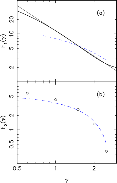
Figure 1.— Dimensionless factors that describe (a) the stellar mass bound to a kicked SMBH (eq. 6) and (b) its effective radius (eq. 17). Thick (black) line in the upper panel is the exact expression derived in Appendix A and thin (black) line is the approximation, given in eq. 8. Open circles in (b) were computed using a Monte-Carlo algorithm. Dashed (blue) lines in both panels show the Dehnen-model approximations of eqs. (15) and (18).

Figure 2.— Evolution of the bound population following a kick; the kick was in the $-\mathbf{X}$ direction at $t=0$. Each frame is centered on the (moving) SMBH. Stars were initially distributed as a power law in density, $\rho\propto r^{-7/4}$; only stars which remain bound following the kick are plotted. Unit of length is $r_{\rm k}$ and frames (a,b,c,d) correspond to times of ($0,10,30,100$) in units of $GM_{\rm BH}/V_{\rm k}^{3}$.

Appendix A presents a computation of the bound mass under these approximations and gives an expression for $F_{1}(\gamma)$ in terms of integrals of simple functions. Figure 1a plots this expression, and also the function

$$F_{1}(\gamma)=11.6\gamma^{-1.75}\,,$$ (8)

which is seen to be an excellent approximation for $0.7\;\hbox to0.0pt{\lower 2.5pt\hbox{$\sim$}\hss}\raise 1.5pt\hbox{$<$}\;\gamma\;\hbox to0.0pt{\lower 2.5pt\hbox{$\sim$}\hss}\raise 1.5pt\hbox{$<$}\;2.5$. (As a check, we computed $F_{1}(\gamma)$ in another way: we generated Monte-Carlo samples of positions and velocities corresponding to an isotropic, power-law distribution of stars around the SMBH prior to the kick and discarded the stars that would be unbound after the kick.) Combining equations (6) and (8), we get

$$f_{\rm b}\approx 11.6\gamma^{-1.75}\left({GM_{\rm BH}\over r_{\bullet}V_{\rm k}^{2}}\right)^{3-\gamma}.$$ (9)

Setting $\gamma=1$ in this expression gives

$$f_{\rm b}\approx 2\times 10^{-4}\left({M_{\rm BH}\over 10^{7}M_{\odot}}\right)^{2}\left({r_{\bullet}\over 10\ {\rm pc}}\right)^{-2}\left({V_{\rm k}\over 10^{3}\ {\rm km\ s}^{-1}}\right)^{-4},$$ (10)

which reproduces reasonably well the values for the bound mass found by Boylan-Kolchin et al. (2004) in their $N$-body simulations of kicked SMBHs; their galaxy models had central power-law density cusps with $\gamma=1$.

Setting $\gamma=1.75$, the value corresponding to a collisional (Bahcall-Wolf) cusp, gives

$$f_{\rm b}\approx 5\times 10^{-3}\left({M_{\rm BH}\over 10^{7}M_{\odot}}\right)^{1.25}\left({r_{\bullet}\over 10\ {\rm pc}}\right)^{-1.25}\left({V_{\rm k}\over 10^{3}\ {\rm km\ s}^{-1}}\right)^{-2.5},$$ (11)

which will be useful in what follows.

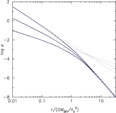
Figure 3.— Steady state, spherically symmetrized density profiles of the bound population for $\gamma=(1,1.5,2)$. Dotted lines show the pre-kick densities; dashed (blue) lines are Dehnen-model fits.

Given the elements of the Keplerian orbits after the kick, the subsequent evolution of the stellar distribution can be computed by simply advancing the positions in time via Kepler’s equation. (Alternately the stellar trajectories can be brute-force integrated; both methods were used as a check.) Figure 2 shows how the bound population evolves from its initially spherical configuration, into a fan-shaped structure at $t\approx 10(GM_{\rm BH}/V_{\rm k}^{3})$, and finally into a reflection-symmetric, elongated spheroid with major axis in the direction of the kick at $t\approx 100(GM_{\rm BH}/V_{\rm k}^{3})$. The latter time is

$$t_{\rm sym}\sim 3\times 10^{3}{\rm yr}\left({M_{\rm BH}\over 10^{7}M_{\odot}}\right)\left({V_{\rm k}\over 1\times 10^{3}\ {\rm km\ s}^{-1}}\right)^{-3}\,,$$ (12)

during which interval the SMBH would travel a distance

$$d_{\rm sym}\sim 3{\rm pc}\left({M_{\rm BH}\over 10^{7}M_{\odot}}\right)\left({V_{\rm k}\over 10^{3}\ {\rm km\ s}^{-1}}\right)^{-2}.$$ (13)

Observing the kick-induced asymmetry would only be possible for a short time after the kick; however the elongation of the bound cloud at $r\gg r_{\rm k}$ would persist indefinitely.

In general, the galactic nucleus might be elongated before the kick, and its major axis will be oriented in some random direction compared with $\mathbf{V}_{\rm k}$. Since the stellar distribution at $r\;\hbox to0.0pt{\lower 2.5pt\hbox{$\sim$}\hss}\raise 1.5pt\hbox{$<$}\;r_{\rm k}$ is nearly unaffected by the kick, the generic result will be a bound population that exhibits a twist in the isophotes at $r\approx r_{\rm k}$ and a radially-varying ellipticity.

Continuing with the same set of approximations made above, we can compute the steady-state distribution of the bound population by fixing the post-kick elements of the Keplerian orbits and randomizing the orbital phases (or equivalently by continuing the integration of Fig. 2 until late times.) The resultant density profiles are shown in Figure 3 for $\gamma=(1,1.5,2)$. Beyond a few $r_{\rm k}$, the spherically-symmetrized density falls off as $\sim r^{-4}$; the stars in this extended envelope move on eccentric orbits that were created by the kick.

It turns out that Dehnen’s (1993) density law:

$$\rho(r)={(3-\gamma)M_{\rm D}\over 4\pi}\xi^{-\gamma}\left(1+\xi\right)^{\gamma-4},\ \ \ \ \xi\equiv r/r_{\rm D}$$ (14)

is a good fit to these density profiles for $1\;\hbox to0.0pt{\lower 2.5pt\hbox{$\sim$}\hss}\raise 1.5pt\hbox{$<$}\;\gamma\;\hbox to0.0pt{\lower 2.5pt\hbox{$\sim$}\hss}\raise 1.5pt\hbox{$<$}\;2$, if $r_{\rm D}$ is set to $2.0r_{\rm k}$; here $M_{\rm D}$ is the total (stellar) mass. Figure 3 shows the Dehnen-model fits as dashed lines. Using the expressions in Dehnen (1993), it is easy to show that the Dehnen models so normalized satisfy

$${M_{\rm D}\over M_{\rm BH}}=2^{4-\gamma}\left({GM_{\rm BH}\over r_{\bullet}V_{\rm k}^{2}}\right)^{3-\gamma}\,,$$ (15)

implying $F_{1}\approx 2^{4-\gamma}$. This alternate expression for $F_{1}$ is plotted as the dashed line in Figure 1a. Unless otherwise stated, we will use equation (8) for $F_{1}$ in what follows.

So far we have assumed that stars remaining bound to the SMBH experience only its point-mass force. In reality, beyond a radius of order $r_{\rm infl}\approx(V_{\rm k}/\sigma)^{2}r_{\rm k}$, stars will also feel a significant acceleration from the combined attraction of the other stars, leading to a tidally truncated density profile at $r\gg r_{\rm k}$. We ignore that complication in what follows.

We note that $r_{\bullet}$ is determined by the density of stars just before the massive binary has coalesced, and may be substantially different from $r_{\rm infl}$ (eq. 3). In the next section we discuss predictions for $r_{\bullet}$ based on a number of models for the evolution of the massive binary prior to the kick.

Before doing so, we first present the mass-radius and mass-velocity dispersion relations for the bound population, expressed in terms of $r_{\bullet}$ as a free parameter.

2.2. Mass-Radius Relation

Combining equations (1) and (6), we get

$${M_{\rm b}\over M_{\rm BH}}=F_{1}(\gamma)\left({r_{\rm k}\over r_{\bullet}}\right)^{3-\gamma}\,.$$ (16)

As a measure of the size of the HCSS, the effective radius $r_{\rm eff}$, i.e. the radius containing one-half of the stellar mass in projection, is preferable to $r_{\rm k}$. We define a second form factor $F_{2}$ such that

$$r_{\rm eff}=F_{2}(\gamma)r_{\rm k}\,.$$ (17)

Figure 1(b) plots $F_{2}(\gamma)$. Also shown by the dashed line is the relation corresponding to the Dehnen-model approximation described above, for which

$$F_{2}(\gamma)\approx 1.5\left(2^{1/(3-\gamma)}-1\right)^{-1}$$ (18)

(Dehnen 1993). The Dehnen model approximation is reasonably good for all $\gamma$ in the range $0.5\leq\gamma\leq 2.5$ and will be used as the default definition for $F_{2}$ in what follows.

Combining equations (16) and (18) gives the mass-radius ($M_{\rm b}-r_{\rm eff}$) relation for HCSS’s, in terms of the (yet unspecified) $r_{\bullet}$:

$$M_{\rm b} = K(\gamma)M_{\rm BH}r_{\bullet}^{\gamma-3}r_{\rm eff}^{3-\gamma},$$ (19a)

$$K(\gamma) \equiv 11.6\gamma^{-1.75}\left[(3/2)(2^{1/(3-\gamma)}-1)^{-1}\right]^{\gamma-3};$$ (19b)

for $\gamma=(1,1.5,2)$, $K=(0.89,1.41,2.32)$.

2.3. Mass-Velocity Dispersion Relation

Stars bound to a recoiling SMBH move within the point-mass potential of the SMBH, for which the local circular velocity is $(GM_{\rm BH}/r)^{1/2}$. The circular velocity at $r=r_{\rm k}$ is just $V_{\rm k}$, so the characteristic (e.g. rms) speed of stars in the bound cloud scales as $V_{\rm k}$, motivating us to define a third form factor $F_{3}$ such that

$$\sigma_{\rm obs}=F_{3}(\gamma)V_{\rm k},$$ (20)

where $\sigma_{\rm obs}$ is the measured velocity dispersion. To the extent that $\gamma$ is known, and/or the dependence of $F_{3}$ on $\gamma$ is weak, it follows that the amplitude of the initial kick can be empirically determined by measuring the velocity dispersion of the stars.

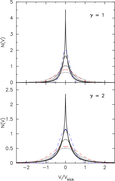
Figure 4.— Line-of-sight distribution of velocities of stars bound to a recoiling SMBH, as seen from a direction perpendicular to the kick. Initially $\rho\propto r^{-\gamma},\gamma=(1,2)$; the phase-space distribution following the kick was computed as in Paper I. Solid curves show $N(V)$ as defined by all bound stars (thick) and progressively thinner curves show $N(V)$ defined by bound stars within a projected distance of $(10,3,1)r_{\rm k}$ from the SMBH. Dashed (blue and red) curves show Gaussian distributions with $\sigma=(0.2,0.5)V_{\rm k}$ ($\gamma=1$) and $\sigma=(0.35,0.75)V_{\rm k}$ ($\gamma=2$) respectively.

An integrated spectrum will include stars at all (projected) radii within the spectrograph slit. (E.g. at the distance of the Virgo cluster, a $1^{\prime\prime}$ slit corresponds to $\sim 80$ pc, larger than $r_{\rm eff}$ for even the largest HCSS’s.) Since $V\sim r^{-1/2}$, the distribution $N(V)$ of line-of-sight velocities of stars within the slit will contain significant contributions from stars moving both much faster and much slower than $V_{\rm k}$ and can be significantly non-Gaussian.

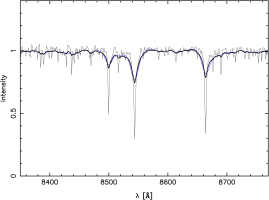
Figure 5.— Absorption line spectrum of the K0III star HR 7615, convolved with two broadening functions. Thick (black) curve: $N(V)$ from the top panel of Fig. 4, computed from the entire bound population, assuming $V_{\rm k}=1000$ km s^-1. Thin (blue) curve: Gaussian $N(V)$ with $\sigma=200$ km s^-1.

Figure 4 shows $N(V)$ for bound clouds with $\gamma=1$ and $2$, as seen from a direction perpendicular to the kick. (This is the a priori most likely direction for observing a prolate object. Since the HCSS is nearly spherical within a few $r_{\rm k}$, the results cited below depend weakly on viewing angle.) Since more than 1/2 of the stars lie at $r>2r_{\rm k}$ and are moving with $v<V_{\rm k}$, the central core of the distribution has an effective width that is much smaller than $V_{\rm k}$; most of the information about the high velocity stars near the SMBH is contained in the extended wings (e.g. van der Marel, 1994).

Velocity dispersions of stellar systems are typically measured by comparing an observed, absorption line spectrum with template spectra that have been broadened with Gaussian $N(V)$’s; the comparison is either made directly in intensity-wavelength space (e.g. Morton & Chevalier, 1973) or via cross-correlation (e.g. Simkin, 1974). For example, internal velocities of UCDs (ultra-compact dwarf galaxies) in the Virgo and Fornax clusters have been determined in both ways (e.g. Hilker et al. 2007; Mieske et al. 2008). Figure 5 shows the results of broadening the spectrum of a K0 star in the CaII triplet region ($8400$Å$\leq\lambda\leq 8800$ Å), with two broadening functions: $N(V)$ from the top panel of Figure 4, scaled to $V_{\rm k}=1000$ km s^-1, and a Gaussian $N(V)$ with $\sigma=200$ km s^-1. The two broadening functions produce similar changes in the template spectrum; the $N(V)$ from the bound cloud generates more ‘peaked’ absorption lines, but this difference would be difficult to see absent very high quality data.

We computed the best-fit, Gaussian $\sigma$ corresponding to the various broadening functions in Figure 4 as a function of $V_{\rm k}$. The stellar template of Figure 5 was convolved with Gaussian $N(V)$’s having $\sigma$ in the range $2$ to $2000$ km s^-1and a step size of $1$ km s^-1. Each of the Gaussian-convolved templates was then compared with the simulated HCSS  spectrum, and the “observed” velocity dispersion $\sigma_{\rm obs}$ was defined as the $\sigma$ for which the Gaussian-convolved template was closest, in a least-squares sense, to the HCSS  spectrum. No noise was added to either the HCSS  or comparison spectra.

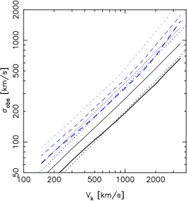
Figure 6.— Velocity dispersions $\sigma_{\rm obs}$ that would be inferred from broadened absorption-line spectra of HCSS’s. Solid (black) lines: $\gamma=1$; dashed (blue) lines: $\gamma=2$, where $\gamma$ is the power-law index of the stellar density profile before the kick. Thick curves correspond to all bound stars; thinner curves correspond to an observing aperture that includes only bound stars within a projected distance $10r_{\rm k}$ and $3r_{\rm k}$ from the SMBH (as viewed from a direction perpendicular to the kick). Dotted lines show $\sigma_{\rm obs}=0.2V_{\rm k}$ and $\sigma_{\rm obs}=0.35V_{\rm k}$.

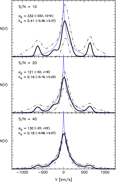
Figure 7.— Recovery of HCSS broadening functions from simulated absorption line spectral data with various amounts of added noise. Blue lines are the input $N(V)$ (from Figure 4, with $\gamma=1$ and $V_{\rm k}=10^{3}$ km s^-1). Solid lines are the recovered $N(V)$s and dash-dotted lines are 90% confidence bands. $\sigma_{0}$ and $h_{4}$ are coefficients of the Gauss-Hermite fit to the recovered $N(V)$; 90% confidence intervals on the parameters are given.

Figure 6 shows the results for $\gamma=(1,2)$, $150$ km s^-1$\leq V_{\rm k}\leq 4000$ km s^-1, and for (circular) apertures of various sizes. When the entire HCSS  is included in the slit, $\sigma_{\rm obs}\approx 0.15V_{\rm k}$ ($\gamma=0.5$), $\approx 0.20V_{\rm k}$ ($\gamma=1$), and $\approx 0.35V_{\rm k}$ ($\gamma=2$). These values are well fit by the ad hoc relation

$$\ln F_{3}=-2.17+0.56\gamma,\ \ \ 0.5\;\hbox to0.0pt{\lower 2.5pt\hbox{$\sim$}\hss}\raise 1.5pt\hbox{$<$}\;\gamma\;\hbox to0.0pt{\lower 2.5pt\hbox{$\sim$}\hss}\raise 1.5pt\hbox{$<$}\;2.$$ (21)

As the aperture is narrowed, $\sigma_{\rm obs}$ increases to values closer to $V_{\rm k}$, although as argued above, realistic slits would be expected to include essentially the entire HCSS and we will assume this in what follows.

We note that some ultra-compact dwarf galaxies (UCDs) have $\sigma_{\rm obs}$ as large as $40-50$ km s^-1and that the implied masses are difficult to reconcile with simple stellar population models, which has led to suggestions that the UCDs are dark-matter dominated (Hilker et al. 2007; Mieske et al. 2008). Alternatively, some UCD’s might be bound by a central black hole; for instance, an observed $\sigma$ of $50$ km s^-1is consistent with an HCSS  produced via a kick of $\sim 250$ km s^-1($\gamma=1$). Detection of the high-velocity wings in $N(V)$ (Fig. 4) could distinguish between these two possibilities.

While spectral deconvolution schemes exist that can do this (e.g. Saha & Williams, 1994; Merritt, 1997), they require high signal-to-noise ratio data. Precisely how high is suggested by Figure 7, which shows the results of simulated recovery of HCSS broadening functions from absorption line spectra. The spectrum of Figure 5 was convolved with the $\gamma=1$ $N(V)$ plotted in Figure 4, with $V_{\rm k}=10^{3}$ km s^-1. Noise was then added to the broadened spectrum (as indicated in the figures by the signal-to-noise ratio S/N) and the broadening function was recovered via a non-parametric algorithm (Merritt, 1997); confidence bands were constructed via the bootstrap. Figure 7 suggests that S/N$\approx 40$ permits a reasonably compelling determination of a non-Gaussian $N(V)$. This conclusion is reinforced by the inferred values of the Gauss-Hermite (GH) moments $\sigma_{0}$ and $h_{4}$; the former measures the width of the Gaussian term in the GH expansion of $N(V)$ while $h_{4}$ measures symmetric deviations from a Gaussian. For S/N$=40$, the recovered $h_{4}=0.18\pm 0.1$ (90%), significantly different from zero. (We note that the velocity dispersion corresponding to the GH expansion is $\sigma_{\rm c}=(1+\sqrt{6}h_{4})\sigma_{0}$ which is close to $\sigma_{\rm obs}$ as defined above.) In §7 we discuss the feasibility of obtaining HCSS spectra with such high S/N.

Combining equations (17) and (20), the (stellar) mass-velocity dispersion ($M_{\rm b}-\sigma_{\rm obs}$) relation for HCSS’s becomes

$${M_{\rm b}\over M_{\odot}}\approx F_{1}(\gamma)\times F_{3}(\gamma)^{2(3-\gamma)}\left({M_{\rm BH}\over M_{\odot}}\right)\left({GM_{\rm BH}\over r_{\bullet}}\right)^{3-\gamma}\sigma_{\rm obs}^{2(\gamma-3)}.$$ (22)

It is tempting (though only order-of-magnitude correct) to write $r_{\bullet}\approx r_{\rm infl}\approx GM_{\rm BH}/\sigma^{2}$, which allows equation (22) to be written

$${M_{\rm b}\over M_{\rm BH}}\approx F_{1}\times F_{3}^{2(3-\gamma)}\left({\sigma_{\rm obs}\over\sigma}\right)^{2(\gamma-3)}.$$ (23)

The dimensionless coefficient in these two expressions is equal to $(3\times 10^{-3},1.2\times 10^{-2},0.4)$ for $\gamma=(0.5,1,2)$.

3. The Pre-Kick Stellar Density

While the linear extent of a HCSS  is determined entirely by $M_{\rm BH}$ and $V_{\rm k}$ (eq. 1), its luminosity and (stellar) mass depend also on the density of stars around the SMBH (i.e. around the massive binary) just prior to the kick. In this section we discuss likely values for the parameters that determine the pre-kick density of stars near the SMBH and the implications for the mass that remains bound after the kick. In a following section we will relate mass to luminosity and color.

Two inspiralling SMBHs first form a bound pair when their separation falls to $\sim r_{\rm infl}\equiv GM_{\rm BH}/\sigma$, the influence radius of the larger hole. This distance is a few parsecs in a galaxy like the Milky Way. The separation between the two SMBHs then drops very rapidly (on a nuclear crossing time scale) to a fraction $\sim 0.1M_{2}/M_{1}$ of $r_{\rm rinfl}$ as the binary kicks out stars on intersecting orbits via the gravitational slingshot (Merritt 2006a, ). Because a massive binary tends to lower the density of stars or gas around it, the two SMBHs may stall at this separation, never coming close enough together ($\;\hbox to0.0pt{\lower 2.5pt\hbox{$\sim$}\hss}\raise 1.5pt\hbox{$<$}\;10^{-3}$ pc) that gravitational wave emission can bring them to full coalescence. This is the “final parsec problem.”

Of course, in order for a kick to occur, the two SMBHs must coalesce, and in a time shorter than $\sim 10$ Gyr. Roughly speaking, this requires that the density of stars or gas near the binary remain high until shortly before coalescence. This implies, in turn, a relatively large mass in stars that can remain bound to the SMBH after the kick, hence a relatively large luminosity for the HCSS  that results.

Converting these vague statements into quantitative estimates of the stellar density just before the kick requires a detailed model for the joint evolution of stars and gas around the shrinking binary. A number of such models have been discussed (see Gualandris & Merritt, 2008, for a review). Here we focus on the two that are perhaps best understood:

• Collisional loss-cone repopulation. If the two-body relaxation time $t_{R}$ in the pre-kick nucleus is sufficiently short, gravitational scattering between stars can continually repopulate orbits that were depleted by the massive binary, allowing it to shrink on a timescale of $\sim t_{R}$ (Yu, 2002). This process can be accelerated if the nucleus contains perturbers that are significantly more massive than stars, e.g. giant molecular clouds (Perets & Alexander, 2008). Repopulation of depleted orbits guarantees that the density of stars near the binary will remain relatively high as the binary shrinks.

• Collisionless loss-cone repopulation. In non-axisymmetric (barred, triaxial or amorphous) galaxies, some orbits are “centrophilic,” passing near the galaxy center each crossing time. This can imply feeding rates to a central binary as large as $\dot{M}\sim G^{-1}\sigma^{3}$ even in the absence of collisional loss-cone repopulation (Merritt & Poon, 2004). Because the total mass on centrophilic orbits can be $\gg M_{\rm BH}$, interaction of the binary with a mass $\sim M_{\rm BH}$ in stars need not imply a significiant decrease in the local density of stars, again implying a large pre-kick density near the binary.

We now discuss these two pathways in more detail and their implications for the pre-kick stellar density near the SMBH.

3.1. Collisional loss-cone repopulation

At the end of the rapid evolutionary phase described above, the binary forms a bound pair with semi-major axis

$$a\approx a_{\rm h}\equiv{q\over(1+q)^{2}}{r_{\rm infl}\over 4}\,,$$ (24)

with $q\equiv M_{2}/M_{1}\leq 1$ the binary mass ratio (e.g. Merritt 2006a, ). Stars on “loss cone” orbits that intersect the binary have already been removed via the gravitational slingshot by this time, and continued evolution of the binary is determined by the rate at which these orbits are repopulated – in this model, via gravitational scattering. Scattering onto loss-cone orbits around a central mass $M_{\rm BH}=M_{1}+M_{2}$ occurs predominantly from stars on eccentric orbits with semi-major axes $\sim r_{\rm infl}$, and the relevant relaxation time is therefore $\sim t_{R}(r_{\rm infl})$. Relaxation times at $r=r_{\rm infl}$ in real galaxies are found to be well correlated with spheroid luminosities (e.g. Figure 4 of Merritt et al. 2007a, ), dropping below $10$ Gyr only in low-luminosity spheroids – roughly speaking, fainter than the bulge of the Milky Way. Such spheroids have velocity dispersions $\;\hbox to0.0pt{\lower 2.5pt\hbox{$\sim$}\hss}\raise 1.5pt\hbox{$<$}\;150$ km s^-1and contain SMBHs with masses $\;\hbox to0.0pt{\lower 2.5pt\hbox{$\sim$}\hss}\raise 1.5pt\hbox{$<$}\;10^{7}M_{\odot}$. Binary SMBHs in more luminous galaxies might still evolve to coalescence via this mechanism, but only if they contain significant populations of perturbers more massive than $\sim M_{\odot}$, e.g. giant molecular clouds or intermediate mass black holes; Perets & Alexander (2008) have argued that this might generically be the case in the remnants of gas-rich galaxy mergers though this model is unlikely to work in gas-poor, old systems like giant elliptical galaxies.

Denoting the semi-major axis of the massive binary by $a(t)$, one finds (Merritt et al. 2007b, )

$${1\over t_{\rm R}(r_{\rm infl})}\left|{a\over\dot{a}}\right|\approx A\ln\left({a_{\rm h}\over a}\right)+B$$ (25)

for $a_{\rm eq}\;\hbox to0.0pt{\lower 2.5pt\hbox{$\sim$}\hss}\raise 1.5pt\hbox{$<$}\;a(t)\;\hbox to0.0pt{\lower 2.5pt\hbox{$\sim$}\hss}\raise 1.5pt\hbox{$<$}\;a_{\rm h}$, where $a_{\rm eq}\approx 10^{-3}r_{\rm infl}$ is the separation at which energy losses due to gravitational wave emission begin to dominate losses due to interaction with stars; ($A,B$) $\approx$ ($0.016,0.08$) with only a weak dependence on binary mass ratio. The elapsed time between $a=a_{\rm h}$ and $a=a_{\rm eq}$ is of order $t_{R}(r_{\rm infl})$.

Figure 8.— Evolving stellar density around a binary SMBH of mass $M_{1}+M_{2}=10^{6}M_{\odot}$ in a spherical galaxy containing $10^{9}$ Solar-mass stars, in the “collisional loss cone repopulation” regime (Merritt et al. 2007b, ). Solid lines show $\rho(r)$ at five different times, between $a(t)\approx a_{\rm h}$ and $a(t)\approx a_{\rm eq}$. The density falls to zero at $r\approx a(t)$ and smaller values of $a$ correspond to later times; total elapsed time is $\sim 0.5t_{R}(r_{\rm infl})$ where $r_{\rm infl}$ is the gravitational influence radius of the massive binary. Dotted line shows the initial (pre-binary) galaxy density and dashed line has the Bahcall-Wolf (1976) slope, $\rho\propto r^{-7/4}$.

Figure 8 shows the evolution of the stellar density around a massive binary as it shrinks from $a\approx a_{\rm h}$ to $a\approx a_{\rm eq}$; the evolution was computed using the Fokker-Planck formalism described in Merritt et al. (2007b). The same gravitational encounters that scatter stars into the binary also drive the distribution of stellar energies toward the Bahcall-Wolf (1976) “zero-flux” form, $\rho\sim r^{-7/4}$, and on the same time scale, $\sim t_{R}(r_{\rm infl})$; as a result, a high density of stars is maintained at radii $a(t)\;\hbox to0.0pt{\lower 2.5pt\hbox{$\sim$}\hss}\raise 1.5pt\hbox{$<$}\;r\;\hbox to0.0pt{\lower 2.5pt\hbox{$\sim$}\hss}\raise 1.5pt\hbox{$<$}\;0.2r_{\rm infl}$. In effect, the inner edge of the cusp follows the binary as the binary shrinks.

Once $a(t)$ drops below $\sim a_{\rm eq}$, the binary “breaks free” of the stars and evolves rapidly toward coalescence, leaving behind a phase-space gap corresponding to orbits with pericenters $\;\hbox to0.0pt{\lower 2.5pt\hbox{$\sim$}\hss}\raise 1.5pt\hbox{$<$}\;a_{\rm eq}$. (In a similar way, evolution of a binary SMBH in response to gravitational waves and gas-dynamical torques leaves behind a gap in the gaseous accretion disk; Milosavljevic & Phinney 2005.) Gravitational scattering will only partially refill this gap in the time between $a=a_{\rm eq}$ and coalescence (Merritt & Wang, 2005). Figure 8 suggests that $a_{\rm eq}\ll(a_{\rm h},r_{\rm infl})$. Merritt et al. (2007b) estimated, based on the same Fokker-Planck model used to construct Figure 8, that

$${a_{\rm eq}\over r_{\rm infl}}\approx(0.20,0.67,2.3,7.8)\times 10^{-3}$$ (26)

for equal-mass binaries with total mass $M_{1}+M_{2}=(10^{5},10^{6},10^{7},10^{8})M_{\odot}$; the numbers in parentheses decrease by $\sim 25\%$ for binaries with $M_{2}/M_{1}=0.1$.

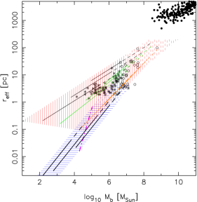
Figure 9.— Effective radius vs. bound stellar mass for HCSSs. Thick solid lines (blue hatched area) are based on the “collisional” loss cone repopulation model and assume a galaxy central velocity dispersion of $\sigma=(50,100,150)$ km s^-1(from left to right). Thin solid lines (red hatched area) are based on the “collisionless” loss cone repopulation model; the three lines in each set assume a galaxy central velocity dispersion of $\sigma=(200,300,400)$ km s^-1(right to left) and the three sets of lines are for $\gamma=0.5$ (black) , 1.0 (green) and 1.5 (orange). For both models, solid lines extend to a maximum $r_{\rm eff}$ based on the assumption that $V_{\rm k}\geq 4.5\sigma$ (escape from the galaxy) while dashed lines correspond to the weaker condition $V_{\rm k}\geq 2\sigma$ (escape from the galaxy core). HCSSs to the left of the dash-dotted (magenta) line are expected to expand appreciably over their lifetime. Data points are from Forbes et al. (2008). Filled circles: E galaxies. Open circles: Ultra-compact Dwarfs (UCDs) and Dwarf-Globular Transition Objects (DGTOs). Stars: globular clusters.

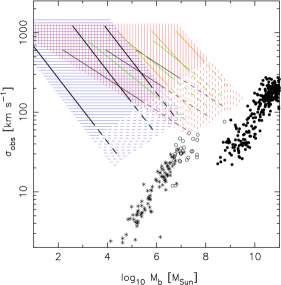
Figure 10.— Observed velocity dispersion vs. bound stellar mass for HCSSs. Thick solid lines (blue hatched area) are based on the “collisional” loss cone repopulation model and assume a galaxy central velocity dispersion of $\sigma=(50,100,150)$ km s^-1(from left to right). Thin solid lines (red hatched area) are based on the “collisionless” loss cone repopulation model; the three lines in each set assume a galaxy central velocity dispersion of $\sigma=(200,300,400)$ km s^-1(right to left) and the three sets of lines are for $\gamma=0.5$ (black) , 1.0 (green) and 1.5 (orange). For both models, solid lines extend to a minimum $\sigma_{\rm obs}$ based on the assumption that $V_{\rm k}\geq 4.5\sigma$ (escape from the galaxy) while dashed lines correspond to the weaker condition $V_{\rm k}\geq 2\sigma$ (escape from the galaxy core). Other symbols are as in Fig. 9.

Following the kick, the density profile of Figure 8 will be truncated beyond $r\approx r_{\rm k}$. The inner cutoff at $r\approx a_{\rm eq}$ satisfies

$${a_{\rm eq}\over r_{\rm k}}\approx 10^{-3}\left({V_{\rm k}\over\sigma}\right)^{2}.$$ (27)

The requirement that $a_{\rm eq}<r_{\rm k}$ – i.e. that at least some stars remain bound after the kick – then becomes $V_{\rm k}\;\hbox to0.0pt{\lower 2.5pt\hbox{$\sim$}\hss}\raise 1.5pt\hbox{$<$}\;30\sigma$, which is never violated by reasonable ($V_{\rm k},\sigma$) values. However, the inner cutoff exceeds $0.1r_{\rm k}$ for $V_{\rm k}\;\hbox to0.0pt{\lower 2.5pt\hbox{$\sim$}\hss}\raise 1.5pt\hbox{$>$}\;10\sigma$, a condition that would be fulfilled for $\sigma=100$ km s^-1and $V_{\rm k}\;\hbox to0.0pt{\lower 2.5pt\hbox{$\sim$}\hss}\raise 1.5pt\hbox{$>$}\;10^{3}$ km s^-1. In what follows we ignore the inner cutoff and assume that the Bahcall-Wolf cusp extends to $r=0$.

The pre-kick density can therefore be approximated as

$$\rho(r)=\left\{\begin{array}[]{lcc}\rho_{0}\left({r\over r_{0}}\right)^{-7/4}&:&0\;\hbox to0.0pt{\lower 2.5pt\hbox{$\sim$}\hss}\raise 1.5pt\hbox{$<$}\;r\;\hbox to0.0pt{\lower 2.5pt\hbox{$\sim$}\hss}\raise 1.5pt\hbox{$<$}\;r_{0}\\ \rho_{0}&:&r_{0}\;\hbox to0.0pt{\lower 2.5pt\hbox{$\sim$}\hss}\raise 1.5pt\hbox{$<$}\;r\;\hbox to0.0pt{\lower 2.5pt\hbox{$\sim$}\hss}\raise 1.5pt\hbox{$<$}\;r_{\rm infl}\end{array}\right.,$$ (28)

where $r_{0}\approx 0.2r_{\rm infl}$ and $\rho_{0}=\rho(r_{0})$ is the density of the galaxy core. Using equations (6) and (28), the mass remaining bound to the coalesced SMBH after a kick is then

$${M_{\rm b}\over M_{\rm BH}} = F_{1}(\gamma)\left({GM_{\rm BH}\over r_{\bullet}V_{\rm k}^{2}}\right)^{3-\gamma}$$ (29a)

$$\approx 1.3\left({GM_{\rm BH}\over r_{\rm infl}V_{\rm k}^{2}}\right)^{5/4}\left({\rho_{0}r_{\rm infl}^{3}\over M_{\rm BH}}\right)$$ (29b)

$$\approx \left({\sigma\over V_{\rm k}}\right)^{5/2}\left({M_{\rm core}\over M_{\rm BH}}\right)\,,$$ (29c)

where $M_{\rm core}\equiv\rho_{0}r_{\rm infl}^{3}$; the last expression assumes $r_{\rm k}<0.2r_{\rm infl}$, i.e. $V_{\rm k}\;\hbox to0.0pt{\lower 2.5pt\hbox{$\sim$}\hss}\raise 1.5pt\hbox{$>$}\;2\sigma$, which is always satisfied for a HCSS that escapes the galaxy core.

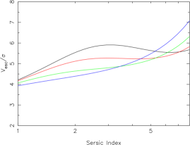
Figure 11.— Escape velocity from the center of a Sersic-law galaxy as a function of Sersic index $n$, in units of the central, projected, 1d velocity dispersion as measured through a circular aperture. Constant mass-to-light ratio was assumed and the effect of the SMBH on the potential or on the motions of stars was ignored in computing $V_{\rm esc}$ and $\sigma$. The four curves (black, red, green, blue) correspond to aperture radii of (0.01,0.03,0.1,0.3) in units of the half-light radius of the galaxy.

To the extent that the galaxy core was itself created by the massive binary during its rapid phase of evolution, then $M_{\rm core}/M_{\rm BH}$ is of order unity (Merritt 2006a, ). (Following the kick, the core will expand still more; Gualandris & Merritt 2008.) Making this assumption yields

$${M_{\rm b}\over M_{\rm BH}}\approx\left({\sigma\over V_{\rm k}}\right)^{5/2}$$ (30a)

$$\approx 2\times 10^{-2}\left({\sigma\over 200\mbox{ km s}^{-1}}\right)^{5/2}\left({V_{\rm k}\over 10^{3}\mbox{ km s}^{-1}}\right)^{-5/2}.$$ (30b)

In the case of ejection from a stellar spheroid like that of the Milky Way ($\sigma\approx 100$ km s^-1, $M_{\rm BH}\approx 4\times 10^{6}M_{\odot}$), we have

$$M_{\rm b}\approx 10^{4}M_{\odot}\left({V_{\rm k}\over 10^{3}{\rm km\ s}^{-1}}\right)^{-5/2},$$ (31)

i.e.

$$3\times 10^{2}\;\hbox to0.0pt{\lower 2.5pt\hbox{$\sim$}\hss}\raise 1.5pt\hbox{$<$}\; M_{\rm b}/M_{\odot} \;\hbox to0.0pt{\lower 2.5pt\hbox{$\sim$}\hss}\raise 1.5pt\hbox{$<$}\;5\times 10^{4},$$ (32a)

$$4000\geq V_{\rm k}/({\rm km\ s}^{-1}) \geq 500.$$ (32b)

Combining equations (1), (17) and (30) gives the mass-radius relation in the collisional regime:

$$M_{\rm b} \approx 0.4G^{-5/4}M_{\rm BH}^{-1/4}\sigma^{5/2}r_{\rm eff}^{5/4}$$ (33c)

$$\approx 4\times 10^{4}M_{\odot}\left({M_{\rm BH}\over 10^{7}M_{\odot}}\right)^{-1/4}\left({\sigma\over 100\ {\rm km\ s}^{-1}}\right)^{5/2}\left({r_{\rm eff}\over 0.1\ {\rm pc}}\right)^{5/4}$$

$$\approx 5\times 10^{4}M_{\odot}\left({\sigma\over 100\ {\rm km\ s}^{-1}}\right)^{1.29}\left({r_{\rm eff}\over 0.1\ {\rm pc}}\right)^{5/4}\,,$$

where the final expression assumes the $M_{\rm BH}-\sigma$ relation in equation (2).

The mass-velocity dispersion ($M_{\rm b}-\sigma_{\rm obs}$) relation for HCSSs follows from equation (30) with $\sigma_{\rm obs}=F_{3}(\gamma)V_{\rm k}\approx 0.30V_{\rm k}$:

$$M_{\rm b} \approx 0.05M_{\rm BH}\sigma^{5/2}\sigma_{\rm obs}^{-5/2}$$ (34a)

$$\approx 2\times 10^{5}M_{\odot}\left({\sigma\over 100\ {\rm km\ s}^{-1}}\right)^{7.4}\left({\sigma_{\rm obs}\over 100\ {\rm km\ s}^{-1}}\right)^{-5/2}$$ (34b)

where the $M_{\rm BH}-\sigma$ relation has again been used.

Figures 9 and 10 plot the relations (33), (34) for $\sigma=(50,100,150)$ km s^-1. Plotted for comparison are samples of globular clusters and dwarf galaxies from the compilation of Forbes et al. (2008).

In these plots, the minimum $r_{\rm eff}$ is presumed to be that associated with a kick of $\sim 4000$ km s^-1. This condition (combined with the $M_{\rm BH}-\sigma$ relation) gives

$$r_{\rm eff}\;\hbox to0.0pt{\lower 2.5pt\hbox{$\sim$}\hss}\raise 1.5pt\hbox{$>$}\;3.0\times 10^{-3}\,{\rm pc}\left({\sigma\over 100\ {\rm km\ s}^{-1}}\right)^{4.86}.$$ (35)

The maximum $r_{\rm eff}$ is associated with the smallest $V_{\rm k}$ that is of physical interest. We express this value of $V_{\rm k}$ as $N\sigma$ which allows us to write

$$r_{\rm eff}\;\hbox to0.0pt{\lower 2.5pt\hbox{$\sim$}\hss}\raise 1.5pt\hbox{$<$}\;4.9\,{\rm pc}\,N^{-2}\left({\sigma\over 100\ {\rm km\ s}^{-1}}\right)^{2.86}.$$ (36)

Kicks large enough to eject a SMBH completely from its galaxy have $N\approx 5$ (Figure 11). Kicks just large enough to remove a SMBH from the galaxy core have $N\approx 2$ (Gualandris & Merritt, 2008). Figures 9 and 10 show the limits on $r_{\rm eff}$ and $\sigma_{\rm obs}$ corresponding to $N=5$ and $N=2$, the latter via dashed lines.

According to Figure 9, HCSSs in this “collisional” regime can have effective radii as big as $\sim 1$ pc when $V_{\rm k}\;\hbox to0.0pt{\lower 2.5pt\hbox{$\sim$}\hss}\raise 1.5pt\hbox{$>$}\;V_{\rm esc}$; on the $M_{\rm b}-r_{\rm eff}$ plane their distribution barely overlaps with globular clusters, and extends to much lower sizes and (stellar) masses. However their velocity dispersions (Fig. 10) would always substantially exceed those of either globular clusters or compact galaxies of comparable (stellar) mass.

3.2. Collisionless loss-cone repopulation

By “collisionless” we mean that the nuclear relaxation time is so long that gravitational scattering can not refill the loss cone of a massive binary at a fast enough rate to significantly affect the binary’s evolution after the hard-binary regime (eq. 24) has been reached. The relevant radius at which to evaluate the relaxation time is $\sim r_{\rm infl}$, the influence radius of the binary (or of the single black hole that subsequently forms). The relaxation time at $r_{\rm infl}$ in elliptical galaxies is found to correlate tightly with $\sigma$ or $M_{\rm BH}$ (Merritt et al. 2007b, ):

$$t_{R}(r_{\rm infl})\approx 8.0\times 10^{9}\ {\rm yr}\left({M_{\rm BH}\over 10^{6}M_{\odot}}\right)^{1.54},$$ (37)

where Solar-mass stars have been assumed. A mass of order $M_{\rm BH}$ is scattered into the central sink in a time $t_{R}(r_{\rm infl})$, and this is also roughly the mass that must interact with the binary in order for it to shrink by a factor of order unity. Even allowing for variance in the phenomenological relations (37), it follows that collisional loss cone refilling is unlikely to significantly affect the evolution of a binary SMBH in galaxies with $\sigma\;\hbox to0.0pt{\lower 2.5pt\hbox{$\sim$}\hss}\raise 1.5pt\hbox{$>$}\;200$ km s^-1or $M_{\rm BH}\;\hbox to0.0pt{\lower 2.5pt\hbox{$\sim$}\hss}\raise 1.5pt\hbox{$>$}\;10^{8}M_{\odot}$.

An alternative pathway exists for stars in these galaxies to interact with a central binary. If the large-scale galaxy potential is non-axisymmetric, a certain fraction of the stellar orbits will have filled centers – these are the (non-resonant) box or centrophilic orbits, which are typically chaotic as well due to the presence of the central point mass (Merritt & Valluri, 1999). Stars on centrophilic orbits pass near the central object once per crossing time; the number of near-center passages that come within a distance $d$ of the central object, per unit of time, is found to scale roughly linearly with $d$ (Gerhard & Binney, 1985; Merritt & Poon, 2004), allowing the rate of supply of stars to a central object to be computed simply given the population of centrophilic orbits. While the latter is not well known for individual galaxies, stable, self-consistent triaxial galaxy models with central black holes can be constructed with chaotic orbit fractions as large as $\sim 70\%$ (Poon & Merritt, 2004). Placing even a few percent of a galaxy’s mass on centrophilic orbits is sufficient to bring two SMBHs to coalescence in 10 Gyr (Merritt & Poon, 2004). Furthermore, the effect of the binary on the density of stars in the galaxy core is likely to be small, since the mass associated with centrophilic orbits is $\gg M_{\rm BH}$ and stars on these orbits spend most of their time far from the center.

Here, we make the simple assumption that the observed core structure of bright elliptical galaxies is similar to what would result from the decay and coalescence of a binary SMBH in the collisionless loss-cone repopulation model. In other words, we assume that the binary SMBHs that were once present in these galaxies did coalesce, and the cores that we now see are relics of the binary evolution that preceded that coalescence. By making these assumptions, we are probably underestimating the density around a SMBH at the time of a kick, since some observed cores will have been enlarged by the kick itself (Gualandris & Merritt, 2008). Also, core sizes in local (spatially resolved) galaxies are likely to reflect a series of past merger events (Merritt 2006a, ); SMBHs that recoiled during a previous generation of mergers would probably have carried a higher density of stars than implied by the current central densities of galaxies.

Above we characterized the pre-kick mass density as $\rho\propto r^{-\gamma}$, with $r_{\bullet}$ the radius at which the enclosed stellar mass equals twice $M_{\rm BH}$. We computed $\gamma$ and $r_{\bullet}$ for a subset of early-type galaxies in the ACS Virgo sample (Côté et al., 2004) for which $\sigma$ was known; for some of these galaxies the SMBH mass has been measured dynamically while $M_{\rm BH}$ in the remaining galaxies was computed from equation (2). Each galaxy was modelled with a PSF-convolved, core-Sersic luminosity profile (Graham et al., 2003), which assumes a power law relation between luminosity density and projected radius inside a break radius $R_{\rm b}$. The core-Sersic fits were numerically deprojected, and converted from a luminosity to a mass density as in Ferrarese et al. (2006). The radius $r_{\bullet}$ was then computed from

$$r_{\bullet}=\left({3-\gamma\over\pi}{M_{\rm BH}\over\rho_{0}r_{0}^{\gamma}}\right)^{1/(3-\gamma)}\,,$$ (38)

with $\gamma$ the central power-law index of the deprojected density; $r_{0}$ is a fiducial radius smaller than $R_{\rm b}$ which we chose to be $1$ pc and $\rho_{0}$ is the mass density at $r=r_{0}$.

Figure 12.— Relation between $r_{\bullet}$, the radius containing a mass in stars equal to twice $M_{\rm BH}$, and central velocity dispersion (top) or black hole mass (bottom), for galaxies in the ACS Virgo sample. Open circles are “core” galaxies; dashed lines are fit to just these points while dotted lines are fit to the entire sample.

Figure 12 shows the relation between $r_{\bullet}$ and $\sigma$ and between $r_{\bullet}$ and $M_{\rm BH}$. “Core” galaxies (those with projected profiles flatter than $\Sigma\propto R^{-0.5}$ near the center) are plotted with open circles and “power-law” galaxies ($\Sigma$ steeper than $R^{-0.5}$) galaxies as filled circles. While this distinction is somewhat arbitrary, Figure 12 confirms that the “core” galaxies have larger $r_{\bullet}$ at given $\sigma$ or $M_{\rm BH}$ than the “power-law” galaxies, consistent with the idea that the central densities of “core” galaxies have been most strongly affected by mergers. The best-fit relations defined by the core galaxies alone are

$$\log_{10}(r_{\bullet}/\rm pc) = -4.84+2.84\log_{10}(\sigma/{\rm km\ s}^{-1})$$ (39a)

$$= -2.92+0.56\log_{10}(M_{\rm BH}/M_{\odot})$$ (39b)

i.e.

$$r_{\bullet} \approx 50\ {\rm pc}\left({\sigma\over 200\ {\rm km\ s}^{-1}}\right)^{2.8}$$ (40a)

$$\approx 35\ {\rm pc}\left({M_{\rm BH}\over 10^{8}M_{\odot}}\right)^{0.56}.$$ (40b)

While these relations are fairly tight, the $\gamma$ values show somewhat more scatter, in the range $0.5\;\hbox to0.0pt{\lower 2.5pt\hbox{$\sim$}\hss}\raise 1.5pt\hbox{$<$}\;\gamma\;\hbox to0.0pt{\lower 2.5pt\hbox{$\sim$}\hss}\raise 1.5pt\hbox{$<$}\;1.5$, and we leave $\gamma$ as a free parameter in what follows.

Combining the relations (40) with equations (19b) and (2) gives a mass-radius relation for HCSSs in the “collisionless” paradigm:

$${M_{\rm b}\over 10^{4}M_{\odot}} \approx G_{\rm s}(\gamma)\left({\sigma\over 200\ {\rm km\ s}^{-1}}\right)^{2.84\gamma-3.66}\left({r_{\rm eff}\over 0.1\ {\rm pc}}\right)^{3-\gamma},$$ (41a)

$$\approx G_{\rm m}(\gamma)\left({M_{\rm BH}\over 10^{8}M_{\odot}}\right)^{0.560\gamma-0.680}\left({r_{\rm eff}\over 0.1\ {\rm pc}}\right)^{3-\gamma},$$ (41b)

where

$$G_{\rm s}(\gamma) = 1.93\times 10^{5}\gamma^{-1.75}\left(750.\over 2^{1/(3-\gamma)}-1\right)^{\gamma-3},$$ (42a)

$$G_{\rm m}(\gamma) = 1.16\times 10^{5}\gamma^{-1.75}\left(525.\over 2^{1/(3-\gamma)}-1\right)^{\gamma-3}.$$ (42b)

Similarly, combining equations (40) with equation (22) gives the mass-velocity dispersion relation:

$${M_{\rm b}\over 10^{4}M_{\odot}} \approx H_{\rm s}(\gamma)\left({\sigma\over 200\ {\rm km\ s}^{-1}}\right)^{10.92-2.02\gamma}\left({\sigma_{\rm obs}\over 100\ {\rm km\ s}^{-1}}\right)^{2(\gamma-3)}$$ (43a)

$$\approx H_{\rm m}(\gamma)\left({M_{\rm BH}\over 10^{8}M_{\odot}}\right)^{2.32-0.44\gamma}\left({\sigma_{\rm obs}\over 100\ {\rm km\ s}^{-1}}\right)^{2(\gamma-3)}$$ (43b)

where

$$H_{\rm s}(\gamma) = 1.92\times 10^{5}\gamma^{-1.75}[1.2F_{3}(\gamma)]^{2(3-\gamma)},$$ (44a)

$$H_{\rm m}(\gamma) = 1.16\times 10^{5}\gamma^{-1.75}[1.1F_{3}(\gamma)]^{2(3-\gamma)}$$ (44b)

and $S(\gamma)$ is given by equation (21).

These relations are plotted in Figures 9 and 10. The allowed locus in the $r_{\rm eff}-M_{\rm b}$ diagram (indicated by red vertical lines) now includes the region occupied also by globular clusters and compact E galaxies. However, velocity dispersions remain much higher than those observed so far in these classes of object.

3.3. Unbound stars

The high, pre-kick stellar densities near the binary which are required for coalescence in the stellar-dynamical models do not necessarily imply that these stars are bound to the SMBH. For instance, in a triaxial galaxy populated by radially-anisotropic box orbits, some of the stars that are momentarily near SMBH will be on orbits that make them unbound with respect to the hole, even before the kick. Another example is loss-cone repopulation by “massive perturbers”; in this model stars are “shot” inward to the binary on eccentric orbits, many with high enough velocities that they would be unbound in the absence of the galactic potential.

When deriving the velocity distribution of stars near the SMBH, we assumed isotropy and we neglected the effect of the galaxy’s gravitational potential on the stellar orbits. These assumptions would be violated in some (though not all) of the loss-cone repopulation mechanisms that have been invoked to solve the stalling problem. Here we discuss briefly the consequences of relaxing these assumptions.

We first note that in the isotropic case, unbound stars are negligibly important. We verified this by constructing fully self-consistent models of galaxies containing SMBHs and counting the unbound stars at each radius. We used (isotropic) Dehnen (1993) models, which have an inner power-law density profile; the self-consistent distribution function describing the stars was computed assuming a central point with mass $M_{\rm BH}=0.002M_{\rm gal}$. We confirmed, for $\gamma=1$ and $\gamma=2$, that the fraction of the mass within $r_{\rm k}$ that is unbound for kick velocities exceeding the escape velocity is never more than a few percent.

If the pre-kick velocity distribution were radially anisotropic, more stars would be unbound with respect to the massive binary and the post-kick bound population would be smaller than what was computed in §2. While this is certainly possible, we note that the anisotropy would have to be appreciable at very small radii, a tenth or hundredth of the SMBH influence radius, in order to substantially affect the fraction of the population that is bound after the kick.

For $\gamma<0.5$, there is no isotropic distribution function that can reproduce the density near the SMBH (or rather, the isotropic distribution function would be negative at highly-bound energies). For such flat cores, one would need to assume a tangentially anisotropic velocity distribution. This would have the effect of increasing the mass of the post-kick bound population, since it would increase the number of stars on low-velocity (nearly circular) orbits at every radius.

These uncertainties deserve to be more completely addressed in a future paper. For now, we prefer to encapsulate them all in the value of $\gamma$.

3.4. Other pathways to coalescence and/or ejection

Recoils large enough to eject SMBHs completely from galaxies can occur even in the absence of gravitational waves, via Newtonian interactions involving three or more massive objects (e.g. Mikkola & Valtonen, 1990; Hoffman and Loeb, 2006). The same interactions can also hasten coalescence of a binary SMBH by inducing changes in its orbital eccentricity. If the infalling SMBH is less massive than either of the components of the pre-existing binary, $M_{3}<(M_{1},M_{2})$, the ultimate outcome is likely to be ejection of the smaller hole and recoil of the binary, with the binary eventually returning to the galaxy center. If $M_{3}>M_{1}$ or $M_{3}>M_{2}$, there will most often be an exchange interaction, with the lightest SMBH ejected and the two most massive SMBHs forming a binary; further interactions then proceed as in the case $M_{3}<(M_{1},M_{2})$. Whether, and to what extent, the ejected SMBH constitutes a HCSS depends on whether it carries a bound population and can retain it during interaction with the other SMBHs. These questions are amenable to high-accuracy $N$-body simulations, which we hope to carry out in the future.

The presence of significant amounts of cold gas in galaxy nuclei can also accelerate the evolution of a binary SMBH. However it is not clear whether the net effect of gas would be to increase, or decrease, the mass of a bound stellar population around the coalesced binary, compared with the purely stellar dynamical estimates made here. On the one hand, gas dynamical torques can lead to rapid formation a tightly-bound binary SMBH (Mayer et al., 2007), reducing the time that the binary can deplete the stellar density in the core on scales of the SMBH influence radii. On the other hand, the formation of a steep Bahcall-Wolf cusp around a shrinking binary discussed in §3 requires that the binary evolution timescale be of order the nuclear relaxation time. Cold gas also implies star formation, which could increase the number of bound stars.

Figure 13.— Evolution of the density around two HCSSs due to resonant scattering of stars into the SMBH’s tidal disruption sphere. Top: $M_{\rm BH}=3\times 10^{6}M_{\odot}$, $M_{\rm b}\approx 7\times 10^{3}M_{\odot}$; bottom: $M_{\rm BH}=3\times 10^{7}M_{\odot}$, $M_{\rm b}\approx 1\times 10^{5}M_{\odot}$; $V_{\rm k}=10^{3}$ km s^-1 in both cases. Left panels show the stellar density at Gyr time increments; the density drops as stars are lost into the SMBH. Right panels show $\dot{N}$.

4. Post-Kick Dynamical Evolution

In the collisional regime, $M_{\rm BH}\;\hbox to0.0pt{\lower 2.5pt\hbox{$\sim$}\hss}\raise 1.5pt\hbox{$<$}\;10^{7}M_{\odot}$, a HCSS will continue to evolve via two-body relaxation after it departs the nucleus. We argued above that the density profile around the SMBH will be close to the “collisionally relaxed” Bahcall-Wolf form, $\rho\propto r^{-7/4}$, at the time of the kick. After the kick, the Bahcall-Wolf cusp is steeply truncated at $r\gtrsim r_{\rm k}$, with $r_{\rm k}\ll r_{\rm infl}$. Gravitational encounters will continue to drive a flux of stars into the tidal disruption sphere of the recoiling SMBH, but because there is no longer a source of stars at $r\approx r_{\rm infl}$ to replace those that are being lost, the density at $r\;\hbox to0.0pt{\lower 2.5pt\hbox{$\sim$}\hss}\raise 1.5pt\hbox{$<$}\;r_{\rm k}$ will steadily drop, at a rate that is determined by the tidal destruction rate. The latter is roughly (Paper I)

$$\dot{N}\approx{\ln\Lambda\over\ln(r_{\rm k}/r_{\rm t})}\left({V_{\rm k}\over r_{\rm k}}\right)f_{\rm b}$$ (45)

stars per unit time, where $r_{\rm t}$ is the tidal disruption radius. Equation (45) is the so-called “resonant relaxation” loss rate (Rauch and Tremaine, 1996) and it differs by a factor $\sim f_{\rm b}^{-1}$ from the standard, non-resonant relaxation rate. In the case of SMBHs embedded in nuclei, most of the disrupted stars come from radii $r\approx r_{\rm infl}$ where resonant relaxation is not effective; once these stars have been removed by the kick, the stars that remain are almost all in the resonant regime and equation (45) is appropriate.

Using equation (45), the condition that significant loss of stars take place in $10^{9}$ yr or less, i.e.

$$\left|{1\over N}{dN\over dt}\right|^{-1}\;\hbox to0.0pt{\lower 2.5pt\hbox{$\sim$}\hss}\raise 1.5pt\hbox{$<$}\;10^{9}{\rm yr},$$ (46)

becomes

$$\left({V_{\rm k}\over 10^{3}{\rm km\ s}^{-1}}\right)^{3/2}\;\hbox to0.0pt{\lower 2.5pt\hbox{$\sim$}\hss}\raise 1.5pt\hbox{$>$}\;{M_{\rm BH}\over 10^{7}M_{\odot}}.$$ (47)

This can be recast as a relation between $M_{\rm b}$ and $r_{\rm eff}$ using the equations in the previous sections; the resulting line is plotted as the magenta dot-dashed curve in Figure 9. HCSSs to the left of this line (in the collisional regime only) should expand appreciably on Gyr timescales.

To simulate the evolution of a HCSS in this regime, we solved the orbit-averaged isotropic Fokker-Planck equation for stars moving in the point-mass potential of a SMBH. In its standard form, based on the non-resonant angular-momentum diffusion coefficients, the Fokker-Planck equation would predict evolution rates that are orders of magnitude too small. Instead we used an approximate resonant diffusion coefficient as in Hopman & Alexander (2006). The amplitude of this diffusion coefficient is not known from first principles and we chose it to approximately reproduce the $N$-body diffusion rates observed in Paper I and Harfst et al. (2008). Unlike in most applications of the Fokker-Planck equation, the outer boundary condition in our case is $f(E=0)=0$, i.e. the density of stars falls to zero far from the SMBH (in addition to being zero near the tidal disruption sphere).

Figure 13 shows the evolution over $10$ Gyr for two HCSSs with $M_{\rm BH}=(3\times 10^{6},3\times 10^{7})M_{\odot}$ and $V_{\rm k}=10^{3}$ km s^-1. The first cluster lies to the left of the magenta dot-dashed line in Figure 9 and the second lies to the right. Tidal disruption rates are initially similar for the two clusters, $10^{-6}{\rm yr}^{-1}\;\hbox to0.0pt{\lower 2.5pt\hbox{$\sim$}\hss}\raise 1.5pt\hbox{$<$}\;\dot{N}\;\hbox to0.0pt{\lower 2.5pt\hbox{$\sim$}\hss}\raise 1.5pt\hbox{$<$}\;10^{-5}{\rm yr}^{-1}$, but the resultant density evolution is much greater in the smaller HCSS since its initial (stellar) mass ($\sim 10^{4}M_{\odot}$) is less. The stellar disruption rates in Figure 13, and their change with time, are similar to estimates made in a simpler way by Paper I.

The expansion seen in Figure 13 is only significant for HCSSs that are older than a few Gyr and that populate the leftmost part of the mass-radius plane (Figure 9). Furthermore, the theory of resonant-relaxation-driven evolution of star clusters is still in a fairly primitive form and the true evolution is likely to be affected in important ways by mass segregation and other effects that have so far hardly been studied. For these reasons we chose to ignore the expansion in what follows; we note here only that the lowest-mass HCSSs are most likely to be affected by the expansion. We hope to return to this topic in more detail in later papers.

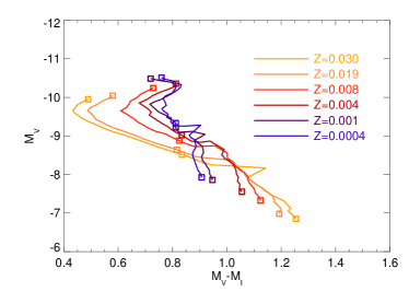
Figure 14.— Color-magnitude diagram of stellar cluster evolution tracks for a range of metallicities and total stellar mass of $10^{5}M_{\odot}$. The clusters evolve from the upper-left to the lower-right, with open squares corresponding to ages of $10^{8}$, $10^{9}$, and $10^{10}$ years.

5. Luminosities and Colors

Given the total stellar mass in the cluster, we calculate the luminosity and color of the object using the tabulated stellar evolution tracks of Girardi et al. (1996). These data give absolute magnitudes in [U,B,V,R,I,J,H,K] bands for a particular stellar (birth) mass, age, and metallicity. We assume that all the stars in the cluster have the same age, and the initial mass function (IMF) is given by a broken power-law distribution (Kroupa, 2001):

$$\phi(M)\propto\left\{\begin{array}[]{lcc}M^{-0.3}&:&0.08M_{\odot}>M\\ M^{-1.3}&:&0.5M_{\odot}>M>0.08M_{\odot}\\ M^{-2.3}&:&M>0.5M_{\odot}\end{array}\right.$$ (48)

At any given time, the total luminosity of a stellar cluster is generally dominated by red giants, yet the additional contributions from the main sequence stars shifts the clusters bluer with respect to individual giants. For example, this means that for a given $B-K$ color, a cluster will have a smaller value of $B-V$ color than an individual giant with the same $B-K$. Thus unresolved HCSSs may be initially distinguished from foreground stars by doing a simple cut in color-color space. Figure 14 shows stellar cluster evolution on a color-magnitude plot, with age progressing from the upper-left ($10^{8}$ years) to the lower-right ($10^{10}$ years). Here we have fixed the total cluster mass at $10^{5}M_{\odot}$, comparable to a typical GC.

If the HCSSs have higher metallicities than typical GCs (a reasonable assumption if the HCSSs are simply displaced nuclei), we expect them to have a significantly wider range of colors, which may be useful in selecting target objects photometrically from a wide field of view. In particular, since the recoiled star clusters are expected to be quite old, they should be particularly red compared to GCs of similar ages.

Given the mass-luminosity relation of any individual HCSS, we can now estimate the luminosity distribution function for a large number of sources. To arrive at an observed source count, we must first begin by calculating the formation rates of HCSSs via SMBH mergers. Since the lifetime of HCSSs is essentially the Hubble time, we need to integrate the cosmological merger history of the universe beginning at large $z$ ($\gtrsim 8$) up until today. While these merger rates are uncertain within at least an order of magnitude, most estimates share the same qualitative behavior, with the merger rates as observed today peaking around redshift $z\approx 2-3$ (Menou et al., 2001; Sesana et al., 2004; Rhook & Whyithe, 2005) and totalling $\sim 10$ mergers per year (as measured by an observer at $z=0$) for $M_{\rm BH}>10^{5}M_{\odot}$.

We follow the results of Sesana et al. (2004) in estimating merger rates as a function of total black hole mass and redshift. In practice, this entails defining an ad-hoc mass distribution function of merging SMBHs with the form

$$\Phi(M,z)\sim f(M)g(z),$$ (49)

where $f(M)$ and $g(z)$ are constructed to match the results of Figure 1 from Sesana et al. (2004). They find that, at any given redshift, the merger rate scales roughly as $M^{-3/2}$ per log mass. This corresponds to a functional form of $f(M)\sim M^{-5/4}$, and $g(z)$ is well-described by a polynomial with an exponential cutoff at large $z$. Then the rate of observed mergers with total mass $M=M_{1}+M_{2}$ is given by

$$R(M,z)=\int\Phi(M_{1},z)\Phi(M_{2},z)dM_{1}.$$ (50)

Figure 15.— Luminosity distribution function of HCSSs per comoving Mpc³. For the collisionless case with $M_{\rm BH}\gtrsim 10^{7}M_{\odot}$, the curves correspond to $\gamma=0.5,1.0,1.5,2.0$: (solid, dotted, dashed, dot-dashed).

Figure 16.— Distribution of observed velocity dispersions $\sigma_{\rm obs}$ for HCSSs with total luminosity $L>10^{4}L_{\odot}$. For the collisionless case with $M_{\rm BH}\gtrsim 10^{7}M_{\odot}$, the curves correspond to $\gamma=0.5,1.0,1.5,2.0$: (solid, dotted, dashed, dot-dashed).

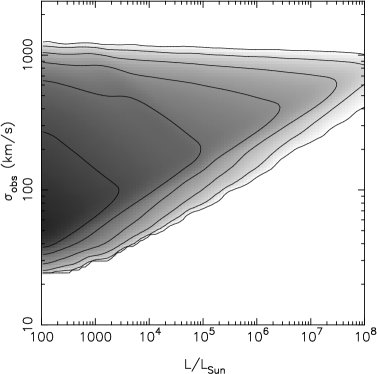
Figure 17.— Number density of HCSSs with a given luminosity and observed velocity dispersion, in units of $d^{2}N/(d\log L\,d\log\sigma)$ per Mpc³, for an age at formation of $10^{8}$ years. The contour lines (from left to right) correspond to values of $\log N=(-2,-3,-4,-5,-6,-7)$.

To model the merger history of the universe, we follow the same approach as in Schnittman & Krolik (2008), integrating forward in time from redshift $z=8$ (using a standard $\Lambda$CDM cosmology with $\Omega_{\rm m}=0.3$, $\Omega_{\Lambda}=0.7$, and $h=0.72$), and at each redshift, generate a Monte Carlo sample of merger pairs, each weighted appropriately from the distribution function $\Phi(M,z)$. We then normalize the total merger rates to reproduce the results of Sesana et al. (2004), as observed today. In the Monte Carlo sampling, we constrain the selected SMBHs to have a mass ratio $q$ greater than $10^{-3}$, motivated by the dynamical friction timescale for the tidal stripping of the satellite to be less than a Hubble time. In any case, the rate at which HCSSs are ejected from the galaxy is not dependent on the precise value of the mass-ratio cutoff, since at mass ratios smaller than $\sim 0.1$, there is little appreciable kick.

For each merger, if the resulting SMBH recoil is large enough to escape from the host galaxy, we consider it to form a HCSS. For a given mass ratio, the kick velocity is calculated using equations (1–4) from Baker et al. (2008), assuming spin magnitudes in the range $0.5\leq a_{\rm 1,2}/M_{\rm 1,2}\leq 1.0$, and spin orientations with a random uniform distribution. These assumptions are reasonable if SMBHs gain most of their mass through accretion (thus a relatively large spin parameter) and come together through dynamical friction after their host galaxies merge (thus random spin orientations). As pointed out by Bogdanovic et al. (2007), gas-rich or “wet” mergers may result in rapid alignment of the two SMBH spins, producing significantly smaller recoils. On the other hand, “dry” mergers should allow the SMBHs to retain their original random orientations (Schnittman, 2004). However, even in wet mergers, a circumbinary disk may form and drive the two SMBHs together via gas-dynamical torque without very much direct accretion onto either SMBH, and therefore remain relatively dry, with correspondingly large kicks.

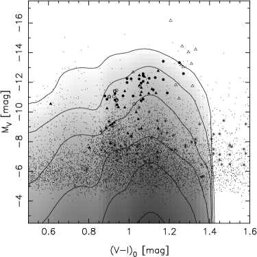
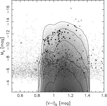
Figure 18.— Number counts of HCSSs with a given $(V-I)$ color and absolute visual magnitude $M_{V}$, in units of $d^{2}N/(dM_{V}\,d(V-I))$ per Mpc³, with the same shading and contour line values as Fig. 17. Top: star formation at $t_{\rm k}-0.1$ Gyr; bottom: star formation at $t_{\rm k}-5$ Gyr. Filled circles are UCD’s from Evstigneeva et al. (2008). Open circles are DGTO’s from Hasegan et al. (2005). Triangles are E-galaxy nuclei from Cote et al. (2006); open triangles are nuclei brighter than $B_{T}=13.5$ and filled triangles are nuclei fainter than $B_{T}=13.5$. Stars are Milky Way GCs from Harris (1996) and points are Virgo cluster GCs from Mieske et al. (2006).

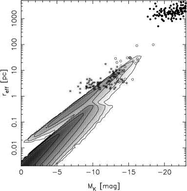
Figure 19.— Number counts of HCSSs with a given effective radius $r_{\rm eff}$ and absolute $K$-magnitude $M_{K}$, in units of $d^{2}N/(d\log r_{\rm eff}\,dM_{K})$ per Mpc³ . Contour levels are the same as in Fig. 17. Data points are from Forbes et al. (2008). Filled circles: E galaxies. Open circles: UCDs and DGTOs. Stars: globular clusters.

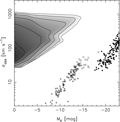
Figure 20.— Number counts of HCSSs with a given velocity dispersion $\sigma_{\rm obs}$ and absolute $K$-magnitude $M_{K}$, in units of $d^{2}N/(d\log\sigma_{\rm obs}\,dM_{K})$ per Mpc³ . Contour levels and data points are the same as in Fig. 17.

6. Rates of Production

From Figure 11, we estimate that the escape velocity is roughly five times the nuclear stellar velocity dispersion $\sigma$, where $\sigma$ is determined from the total SMBH mass from equation (2) above. If the final SMBH does escape, it will carry along a total mass $M_{\rm b}$ in bound stars, determined by equations (34) for collisional relaxation ($M_{\rm BH}\lesssim 10^{7}M_{\odot}$) and (43) for collisionless relaxation ($M_{\rm BH}\gtrsim 10^{7}M_{\odot}$). Neglecting mass loss from stellar winds and tidal disruptions, the total cluster mass in stars should remain roughly constant over a Hubble time. We used the stellar evolution tables from Girardi et al. (1996) to calculate the colors and luminosity of each ejected HCSS for two cluster ages: (1) the stars in the cluster were formed $10^{8}$ years before SMBH merger and ejection, and (2) the stars formed $5\times 10^{9}$ years before ejection. We carried out this exercise both with a single (solar) metallicity for all HCSSs, and also assuming a Gaussian distribution of metallicities:

$$N(x) = {1\over\sqrt{2\pi}\sigma}\exp\left[-\left(x-\overline{x}\right)^{2}/2\sigma^{2}\right],$$ (51a)

$$x \equiv \log_{10}\left[{Z_{i}\over Z_{\odot}}\right].$$ (51b)

We took

$$\overline{x}=-0.5,\ \ \ \ \sigma=0.5$$ (52)

which correspond approximately to what Coté et al. (2006) inferred as the metallicity distribution of nuclear star clusters in the Virgo cluster galaxies, assuming ages of 5 Gyr. We obtained very similar results under the two assumptions, in part because the Girardi et al. (1996) tables only extend to slightly super-solar metallicities ($Z=0.03$). Figures 15–17 assume solar metallicity while Figures 18– 20 assume the metallicity distribution of equation (51).

Figure 15 shows the luminosity distribution function (number per comoving Mpc³) for a range of $\gamma$, with a stellar age of $10^{8}$ yr at time of SMBH recoil. The high-luminosity systems correspond to high-mass SMBHs that merge via collisionless relaxation and thus the number of bound stars is directly a function of the parameter $\gamma$. In Figure 16 we plot the distribution as a function of observed velocity dispersion, limited only to systems with $L>10^{4}L_{\odot}$. The low-velocity cutoff is directly a function of the minimum SMBH mass needed to keep roughly $10^{4}M_{\odot}$ in bound stars; any galactic halo with SMBH mass above $\sim 10^{6}M_{\odot}$ will have an escape velocity $\gtrsim 400$ km/s, and thus an observed velocity dispersion $\sigma_{\rm obs}\gtrsim 120$ km/s. The high-velocity cutoff is defined by the maximum kick velocity of $V_{\rm kick}\lesssim 4000$ km/s, as determined by numerical simulations of BH mergers. While the majority of HCSSs will have small velocity dispersions, the brightest, most massive ones will likely come from the most massive host galaxies, and thus require the largest kicks, in turn giving the highest internal velocity dispersions. In this regard, HCSSs behave similarly to more classical stellar systems: higher masses have higher dispersion. However, holding the SMBH mass fixed, a larger recoil velocity will result in a smaller number of bound stars [eqns. (34, 43)], and thus lower luminosity for higher velocity dispersion.

In Figure 17 we show a contour plot of the density of HCSSs as a function of luminosity and observed velocity dispersion. Here we clearly see that the most luminous systems will also have the largest dispersion, roughly an order of magnitude greater than any globular cluster of the same stellar mass. We can also use Figure 17 to estimate the number of HCSSs that might be observable in the local universe. Assuming a uniform spatial distribution in the local universe, out to a distance of 20 Mpc ($\sim$30,000 Mpc³), for $\gamma=1$ we should expect to see dozens of objects with $L>10^{4}L_{\odot}$ and at least a few with $L>10^{5}L_{\odot}$. However, an all-sky survey to find these few innocuous objects could be prohibitively expensive. Coincidentally, the total mass in the Virgo cluster out to a radius of $\sim 2$ Mpc is roughly the same as that of a smooth universe out to $\sim 20$ Mpc, which is approximately the distance to Virgo (Fouque et al., 2001). In other words, a focused survey of Virgo would be able to sample an effective volume of $\sim 30,000$ Mpc³ all at the same distance and with a relatively small field of view.

We expect to find $\sim 1$ HCSS in Virgo with $m_{K}\leq 20$; $\sim 6$ with $m_{K}\leq 22$; $\sim 40$ with $m_{K}\leq 24$; and $\sim 150$ with $m_{K}\leq 26$, almost all of which would have $\sigma_{\rm obs}\gtrsim 200$ km s^-1. For the Fornax cluster, which is at roughly the same distance, but contains less mass by a factor of $\sim 15$ (Drinkwater et al., 2001), the source counts at the same fluxes should be down by a comparable factor. The Coma cluster, on the other hand, has a mass comparable to Virgo (Kubo et al., 2007), but at a distance of $\sim 100$ Mpc, the apparent brightness of any HCSSs will be smaller by $\sim 4$ magnitudes.

Figures 18, 19 and 20 show predicted number counts in the color-magnitude, size-magnitude, and velocity dispersion-magnitude planes. Over-plotted for comparison are data for other compact stellar systems, from various sources, as discussed in the figure captions. In constructing these figures (as well as Figure 17), we set $\gamma=1$ in the “collisionless” regime. This resulted in a slight bimodality in the distributions corresponding to the discontinuous change in $\gamma$ from $1.75$ to $1$ at galaxy masses of $\sim 10^{11}M_{\odot}$. Alternatively, one could allow $\gamma$ to vary in some smooth way with galaxy mass (cf. the discussion in §3.2).

7. Identifying HCSSs

7.1. Search Strategies

We have shown that stars bound to a recoiling SMBH would appear as very compact stellar clusters with exceptionally high velocity dispersions. The density of HCSSs, and therefore the chances of finding them, will be highest in clusters of galaxies, and nearby galaxy clusters like Virgo and Fornax are therefore well suited to searching for HCSSs.

In their properties, HCSSs share similarities with globular clusters (GCs). However, they would differ from classical GCs by their much larger velocity dispersions and (possibly) higher metal abundances (the nuclei of elliptical galaxies in the Virgo and Coma clusters often have metal abundances comparable with solar, and the cores of quasars, powered by major mergers, frequently show super-solar metallicities). They would differ from stripped galactic nuclei and ultracompact dwarf galaxies (UCDs, Phillips et al. 2001) by their typically greater compactness (Figure 19). They would differ from objects in their local environment by possibly showing a large velocity offset.

How can we find HCSSs and distinguish them from other source populations? Systematic searches would be based on color, compactness, spectral properties, or combinations of these.

Imaging searches for compact stellar systems have been or are currently being carried out, focussing especially on the nearest clusters of galaxies Fornax (e.g. Hilker et al., 1999; Drinkwater et al., 2003; Mieske et al., 2008), Virgo (e.g. Côté et al., 2004; Haşegan et al., 2005; Mieske et al., 2006; Firth et al., 2008), and Coma (Carter et al., 2008), and on a number of nearby groups (Evstigneeva et al., 2007). These studies have resulted in the detection of a large number of GCs, and of several UCDs per galaxy cluster.

Two strategies suggest themselves for identifying HCSSs among existing surveys of compact stellar systems in nearby galaxy clusters. One would focus on the faintest HCSSs which are most abundant; the other would concentrate on the brightest objects, which are rare, but most amenable to follow-up spectroscopic observations.

According to Figure 19, HCSSs separate in $r_{\rm eff}-$luminosity space most strongly at the smallest effective radii, smaller than Galactic GCs, while Figure 18 suggests that their colors should be comparable to (metal rich) GCs or (gas-poor, i.e. non-star-forming, and non-accreting) galactic nuclei. PSF-deconvolved HST imaging can achieve a spatial resolution better than $0.1$ arcsec, corresponding to spatial scales of $\sim 10$ pc at the distance of the Virgo cluster. However, in order to confirm such HCSS candidates, a laborious spectroscopic multi-fiber follow-up survey would then have to be carried out.

Instead, selecting brighter (even though rarer) objects appears more promising and would substantially reduce the exposure time. A key signature of a HCSS is its large velocity dispersion, which would distinguish it from luminous GCs and most known UCDs. At the same time, the highest velocity dispersions would tend to put the broadened absorption lines below the noise. Therefore, HCSSs with $\sigma_{\rm obs}$ below several hundred km s^-1 might be easiest to detect. These are in fact expected to be the most common (Figure 16).

In order to estimate exposure times, we simulated spectra with the multi-object spectrograph FLAMES attached to the VLT (Pasquini et al., 2002), using the spectrograph GIRAFFE in MEDUSA mode. This spectrograph allows the observation of up to 130 targets at a time at intermediate ($\sim 30$ km s^-1) to high ($\sim 10$ km s^-1) spectral resolution. The simulated spectral deconvolutions in §2 suggest that a signal-to-noise (S/N) ratio of $\sim 10$ is sufficient to detect the broadened lines, while S/N $\approx 30$ is desirable in order to probe the non-Gaussianity of the broadening function. In order to reach a S/N of 30 for a cluster of $m_{V}\approx 21$ or fainter ($M_{V}\;\hbox to0.0pt{\lower 2.5pt\hbox{$\sim$}\hss}\raise 1.5pt\hbox{$>$}\;-10$ at Virgo) requires excessive integration times in the high resolution mode. In lower resolution mode, about 10 hours exposure time are required to reach S/N=30 for $m_{V}=20$. Simply detecting the high velocity dispersion requires less time, of order an hour or less for $m_{V}\;\hbox to0.0pt{\lower 2.5pt\hbox{$\sim$}\hss}\raise 1.5pt\hbox{$<$}\;21$.

7.2. Could UCDs be HCSSs?

HCSSs share some properties with UCDs and dwarf-globular transition objects (“DGTOs”; Hasegan et al. 2005). These are compact stellar systems with stellar velocity dispersions as high as $\sim$50 km s^-1, masses between 10^6-8 $M_{\odot}$ and unusually high mass-to-light ratios (e.g. Hilker et al., 2008). Figures 9 and 19 suggest that UCD sizes are consistent with those of the largest (“collisionless”) HCSSs, although Figures 10 and 20 suggest that known UCD velocity dispersions are too low by a factor of at least a few. Furthermore Figures 19 and  20 suggest that HCSSs with properties similar to those of UCDs are likely to be rare. However, there is increasing evidence that UCDs are a “mixed bag” (e.g., Hilker 2006), possibly requiring a number of different formatios mechanisms (Oh et al., 1995; Fellhauer & Kroupa, 2002; Bekki et al., 2003; Mieske et al., 2004; Martini & Ho, 2004; Goerdt et al., 2008). Individual HCSSs might therefore hide among the UCD population, and low-mass UCD and DGTO candidates identified in current and future surveys might sometimes be recoiling HCSSs. Objects like Z2109 (Zepf et al., 2008) with its very unusual and broad [OIII] emission line are also possible candidates.

7.3. Very young HCSSs?

The predicted HCSS colors and luminosities summarized in Figures 18 - 20 reflect the properties of the old ($\sim 5$ Gyr) stellar populations that predominate in our models. A HCSS that was discovered near its birthplace might appear much younger than implied by these plots, particularly if it was born in a starburst galaxy resulting from a merger. The light from such a HCSS might be dominated by young massive stars, at least during the $\sim 0.1-1$ Gyr required for it to exit the galaxy. (We are assuming here that massive stars can form, or at least quickly find their way, well inside the SMBH influence radius, as appears to be the case at the center of the Milky Way. We are further assuming that the recoiling SMBH is not accreting at the time of observation since otherwise the quasar might outshine the starlight.) We implicitly excluded this possibility above by assuming $0.1$ Gyr as a minimum lag between star formation and SMBH ejection.

Starting roughly 6 Myr after a starburst episode, luminosities and colors of the burst population are expected to increase rapidly due to red supergiant stars (RSGs), which begin to appear when main sequence stars of initial mass $\sim 25M_{\odot}$ finish core-hydrogen burning. The absolute magnitude of a burst population with standard initial mass function spikes roughly $\sim 10$ Myr after the burst due to the RSGs; the increase is greatest in the IR bands. For example, in the K band, integrated luminosity increases to a value $\sim 100$ times greater than for the same population at $1$ Gyr (Leitherer et al. 1999) before falling off rapidly after $\sim 14$ Myr. Integrated colors reach their reddest values at the same time, i.e. V-I $\approx 1.5$. Single RSG stars can approach luminosities of $10^{5}-10^{6}L_{\odot}$ (Davies et al. 2007), so the luminosity and color of an HCSS containing $\ll 10^{6}$ stars could undergo enormous relative changes around this time.

There are both advantages and disadvantages to targetting such young HCSSs as a search strategy. (Super)star clusters are commonly found in the centers of starburst galaxies and merger remnants (e.g. Max et al., 2005; Galliano et al., 2008), so in any search based solely on imaging photometry, HCSSs could not be easily distinguished. However, once a HCSS reaches larger separations from the center of the galaxy, it will already deviate from its surroundings by plausibly showing higher metal abundance. On the other hand, even low-resolution spectroscopy could immediately reveal a high velocity relative to the galaxy core or relative to other clusters in the galaxy.

We note that discovery of a young HCSS that is still uniquely associated with its host galaxy can provide important constraints on the time scale associated with late evolution of the binary SMBH that engendered the kick. If coalescence was rapid, the host galaxy of the HCSS will still show signs of recent interaction (for instance tidal tails). If the massive binary stalled for $\;\hbox to0.0pt{\lower 2.5pt\hbox{$\sim$}\hss}\raise 1.5pt\hbox{$>$}\;10^{8}-10^{9}$ yr before coalescing, these signs will be mostly gone. Age dating of the recoil event could be based on (projected) distance from the galaxy core and recoil velocity, and/or on the age of the stellar populations.

7.4. Exotic manifestations

HCSSs with accreting central black holes, powered either by stellar tidal disruptions or stellar mass loss, were discussed in Paper I. This sub-population could be efficiently searched for by combining optical properties with information from multi-wavelength surveys, e.g., in the X-ray, UV or radio band. We speculate that the unusual optical transient source SCP06F6 (Barbary et al., 2008) might be a tidally-detonated white dwarf bound to a recoiling SMBH (as discussed already in Paper I). This scenario would fit the high amplitude of variability of the transient, the absence of an obvious host galaxy, and the possible association with a cluster of galaxies at $z=1.1$. However, the observed symmetry of the lightcurve might suggest a lensing origin (Barbary et al., 2008). The unusual optical spectrum of this source could be caused by the tidal-debris disk illuminating the outer disk or the outflowing part of the detonation debris. That way, the observed extreme, unusally broadened absorption features would be caused if we are looking down-stream. Gaensicke et al. (2008) recently reported the detection of an X-ray source co-incident with SCP 06F6 with an X-ray luminosity at the lower end of known tidal disruption flares (Komossa et al., 2004). These authors discuss supernoave-related scenarios but also consider tidal disruption of a star, and suggest a preliminary redshift of 0.14, in which case the source is not associated with the cluster at redshift 1.1.

Finally, some of the oldest surviving HCSSs would consist mostly of stellar end states. They would be quite faint, since only very low-mass stars and WDs would remain, but could possibly be identified by their very unusual colors.

8. The Inverse Problem

We have focused on the “forward” problem of predicting the numbers and properties of HCSSs given reasonable assumptions about the distribution of gravitational wave kicks and the merger history of the universe. Once HCSSs have been detected, one can begin work on the potentially more interesting inverse problem: using the measured properties of HCSSs  to infer the distribution of GW kicks and its evolution over time.

The inverse problem is made easier by the remarkable property of HCSSs (§2) that they encode the magnitude of their natal kick in their spectra. Measuring the degree to which the absorption-line spectrum of a HCSS has been broadened by internal stellar motions leads immediately to an estimate of $V_{\rm k}$. Such a measurement is completely independent of the space velocity of the HCSS at the moment of observation. It is reasonably independent of the initial (pre-kick) density profile, and it depends on the the time since the kick only to the extent that the HCSS changes its structure over time; such changes are expected to be small for the brightest HCSSs(§4).

For a “collisional” ($M_{\rm BH}\;\hbox to0.0pt{\lower 2.5pt\hbox{$\sim$}\hss}\raise 1.5pt\hbox{$<$}\;10^{7}M_{\odot}$) HCSS, with $\gamma\approx 1.75$, equation (21) gives

$$\ln F_{3}=-2.17+0.56\times 1.75,$$ (53)

i.e.

$$V_{\rm k}\approx 3.3\sigma_{\rm obs}.$$ (54)

Absent any knowledge about the internal structure of the HCSS, the coefficient in equation (54) is uncertain, but not greatly so. Allowing the inner density profile slope to vary over the range $1\leq\gamma\leq 2$ implies

$$2.9\;\hbox to0.0pt{\lower 2.5pt\hbox{$\sim$}\hss}\raise 1.5pt\hbox{$<$}\;V_{\rm k}/\sigma_{\rm obs}\;\hbox to0.0pt{\lower 2.5pt\hbox{$\sim$}\hss}\raise 1.5pt\hbox{$<$}\;5.0.$$ (55)

If more information about the HCSS is available than just $\sigma_{\rm obs}$, this estimate of $V_{\rm k}$ could be refined, to a degree that depends on the size and distance of the HCSS and on the access to observing time: (1) A deep spectrum would allow extraction of the stellar broadening function $N(V)$, as in Figure 7. $N(V)$ contains more information about the spatial and velocity distribution of stars around the SMBH than $\sigma_{\rm obs}$ alone (e.g. Merritt, 1993). (2) If the HCSS is near enough and/or large enough to be spatially resolved, constraints can be put on the slope of the stellar density profile from the photometry.

Measuring both $r_{\rm k}$ and $V_{\rm k}$ gives $M_{\rm BH}$ (eq. 1), allowing one to investigate the dependence of kick velocity on SMBH mass, and (via the $M_{\rm BH}-\sigma$ relation) on galaxy mass. Combined with the total light of the HCSS  and perhaps with a mass-to-light ratio derived from broad-band colors, $r_{\rm k}$ and $M_{\rm BH}$ give an estimate of the pre-kick nuclear density via equation (6).

Most detected HCSSs may be spatially unresolved. Even in this case, broad-band magnitudes would allow a sample of HCSSs to be placed on the color-magnitude or velocity dispersion-magnitude diagrams (Figs. 19, 20). The number of detected HCSSs per unit volume combined with their distribution over these observational planes contains information about the time-integrated ejection rate, hence the galaxy merger rate. Colors would also provide an indirect constraint on the time since the kick.

So far we have emphasized kicks large enough to unbind SMBHs from galaxies, $V_{\rm k}\;\hbox to0.0pt{\lower 2.5pt\hbox{$\sim$}\hss}\raise 1.5pt\hbox{$>$}\;500$ km s^-1 (Merritt et al., 2004). If these are the only objects detected as HCSSs  then they will contain information only about the high-$V_{\rm k}$ part of the kick distribution (although we note that a large fraction of kicks may be above 500 km s^-1). Many kicks will fall below galactic escape velocities, particularly in the largest galaxies, producing HCSSs that oscillate about the core or drift for long times in the envelope (Madau and Quataert, 2004; Gualandris & Merritt, 2008). Since the size of a HCSS scales inversely with its kick (eq. 1), such objects would be among the largest and brightest HCSSs, but detection might be difficult since they would be superposed on or behind the image of the galaxy. Such HCSSs would also have finite lifetimes before finding their way back to the center of the galaxy.

9. Conclusions

1. Supermassive black holes (SMBHs) kicked out from the centers of galaxies by gravitational wave recoil are accompanied by a cluster of bound stars with mass $\sim 10^{-2}$ times the black hole mass or less, and radius $\sim 10^{1}$ pc or less – a “hyper-compact stellar system” (HCSS).

2. HCSSs have density profiles that can uniquely be calculated given the kick velocity and given the stellar distribution prior to the kick. The density at large distances from the SMBH falls off as $\sim r^{-4}$.

3. Internal (rms) velocities of HCSSs are very high, $\sim 10^{2}-10^{3}$ km s^-1, and comparable to their kick velocities. Their overall velocity distributions are extremely non-Gaussian.

4. HCSSs could be distinguished photometrically from foreground red giants, based on their bluer (lower) values of $B-V$ for a given $B-K$. They also should appear redder than low-metallicity GCs with comparable ages $\gtrsim 1$ Gyr.

5. With a simplified cosmological merger model, we are able to estimate expected number counts and luminosity distributions of HCSSs in the local universe. Detection of perhaps $10^{2}$ HCSSs should be possible in the Virgo cluster alone, although only a few may be bright enough to allow high S/N spectroscopy and provide solid confirmation of their extreme velocity dispersions.

6. Some HCSSs may already exist in survey data of compact stellar sysetms in the Fornax, Virgo and Coma galaxy clusters.

7. Because the kick velocity of a HCSS is related in a simple way to its measured velocity dispersion, the distribution of gravitational wave kicks can be empirically determined from a sufficiently large sample of HCSSs.

Paper I (Komossa & Merritt 2008a, ) first derived the basic properties of HCSSs  including their compactness and high internal velocity dispersions, and presented a possible route to detection via off-nuclear tidal disruption flares. The current paper derives the intrinsic properties of HCSSs in a more complete and general way and relates those properties to the properties of the host galaxy. Together, these two papers complement the growing number of recent papers that discuss gas-related signatures of gravitational wave recoil. While this paper was being submitted, we learned of a related work by O’Leary & Loeb (2009) which argues that many thousands of low-mass HCSSs should be present in the Milky Way halo.

$$f_{0}(E)=C\left|2E\right|^{\gamma-3/2},\ \ \ \ -\infty\leq 2E\leq 0\,$$ (1)

where $E=V^{2}/2-GM_{\rm BH}/r$ is the energy per unit mass of a star. The pre-kick stellar density is $\rho_{0}(r)\propto r^{-\gamma}$. As above, we ignore the contribution to the gravitational potential from the stars.

Immediately after the kick, transfer to a frame moving with the SMBH. Assume without loss of generality that the kick is along the $x$ axis. In this frame, the phase space density is

$$f=C\left[{2GM_{\rm BH}\over r}-\left(V_{x}-V_{\rm k}\right)^{2}-V_{y}^{2}-V_{z}^{2}\right]^{\gamma-3/2}$$ (2)

in the velocity-space region that lies within the spere

$$\left(V_{x}-V_{\rm k}\right)^{2}+V_{y}^{2}+V_{z}^{2}=2{GM_{\rm BH}\over r}$$ (3)

and zero elsewhere.

Stars are bound to the SMBH after the kick if they lie within the sphere

$$V_{x}^{2}+V_{y}^{2}+V_{z}^{2}=2{GM_{\rm BH}\over r}.$$ (4)

The intersection of the surface of this sphere, and the surface of the sphere defined by equation (3), defines a circle of radius $\left[2GM_{\rm BH}/r-\left(V_{\rm k}/2\right)^{2}\right]^{1/2}$ with center on the $V_{x}$-axis at $V_{x}=V_{\rm k}/2\equiv V_{0}$ (Figure 21a).

The configuration-space density of the bound stars is then

$$\rho_{\rm k}(r)=2\pi C\int dV_{x}\int dV_{t}\ V_{t}\left[{2GM_{\rm BH}\over r}-\left(V_{x}-V_{\rm k}\right)^{2}-V_{t}^{2}\right]^{\gamma-3/2}\,,$$ (5)

where the velocity-space volume element has been written $d^{3}V=2\pi dV_{x}V_{t}dV_{t}$, $V_{t}^{2}\equiv V_{y}^{2}+V_{z}^{2}$, and the region of integration extends over the volume enclosed by the intersection of the two spheres in Figure 21a.

Define new variables

$$x={V_{x}-V_{\rm k}\over\sqrt{2GM_{\rm BH}/r}},\ \ \ \ y={V_{t}^{2}\over 2GM_{\rm BH}/r}.$$ (6)

The contribution to $\rho_{\rm k}(r)$ from the velocity-space region to the left of the dotted curve in Figure 21a (i.e. $V_{x}\leq V_{0}$) is

$$\rho_{I}(r) = \pi C\left({2GM_{\rm BH}\over r}\right)^{\gamma}\int_{-1}^{-\sqrt{r/8r_{\rm k}}}dx\int_{0}^{1-x^{2}}dy\left(1-x^{2}-y\right)^{\gamma-3/2}$$ (7a)

$$= {\pi C\over\gamma-1/2}\left({2GM_{\rm BH}\over r}\right)^{\gamma}\int_{\sqrt{r/8r_{\rm k}}}^{1}dx\left(1-x^{2}\right)^{\gamma-1/2}\,,$$ (7b)

where $r_{\rm k}\equiv GM_{\rm BH}/V_{\rm k}^{2}$ as above; $\rho_{I}=0$ for $r>8r_{\rm k}$. The contribution to $\rho_{\rm k}(r)$ from the velocity-space region to the right of the dotted curve in Figure 21a (i.e. $V_{x}>V_{0}$) is

$$\rho_{II}(r) = \pi C\left({2GM_{\rm BH}\over r}\right)^{\gamma}\int_{-\sqrt{r/8r_{\rm k}}}^{1-\sqrt{r/2r_{\rm k}}}dx\int_{0}^{1-x^{2}-r/2r_{\rm k}-2x\sqrt{r/2r_{\rm k}}}dy\left(1-x^{2}-y\right)^{\gamma-3/2}$$ (8a)

$$= {\pi C\over\gamma-1/2}\left({2GM_{\rm BH}\over r}\right)^{\gamma}\int_{-\sqrt{r/8r_{\rm k}}}^{1-\sqrt{r/2r_{\rm k}}}dx\left[\left(1-x^{2}\right)^{\gamma-1/2}-\left({2r\over r_{\rm k}}\right)^{\left(\gamma-1/2\right)/2}\left(\sqrt{r\over 8r_{\rm k}}+x\right)^{\gamma-1/2}\right].$$ (8b)

Figure 21.— (a) Illustrating the velocity-space region occupied by stars at radius $r$ around a kicked SMBH, in a frame moving with the kick velocity. Stars that remain bound after the kick lie in the region of intersection of the two spheres. Solid lines show the density of bound stars around a kicked SMBH, immediately after the kick, for four different values of the pre-kick density slope, $\gamma=(0.5,1,1.5,2)$ (dotted lines). (b) Solid lines show the density of bound stars around a kicked SMBH, immediately after the kick, for four different values of the pre-kick density slope, $\gamma=(0.5,1,1.5,2)$ (dotted lines).

Summing $\rho_{I}(r)$ and $\rho_{II}(r)$, and fixing $C$ by the requirement that the post-kick density in the limit $V_{\rm k}\rightarrow 0$ equal the pre-kick density $\rho_{0}(r)$:

$$\rho_{0}(r)={3-\gamma\over 2\pi}{M_{\rm BH}\over r_{\bullet}^{3}}\left({r\over r_{\bullet}}\right)^{-\gamma},$$ (9)

yields

$$\rho_{\rm k}(r) = {3-\gamma\over 2\pi I_{1}(\gamma,0)}{M_{\rm BH}\over r_{\bullet}^{3}}\left({r\over r_{\bullet}}\right)^{-\gamma}\left[I_{1}\left(\gamma,r\right)-\left({2r\over r_{\rm k}}\right)^{\left(\gamma-1/2\right)/2}I_{2}\left(\gamma,r\right)\right],\ \ \ \ r\leq 8r_{\rm k}$$ (10a)

$$I_{1}\left(\gamma,r\right) = \int_{\sqrt{r/2r_{\rm k}}-1}^{1}dx\left(1-x^{2}\right)^{\gamma-1/2},$$ (10b)

$$I_{2}\left(\gamma,r\right) = \int_{-\sqrt{r/8r_{\rm k}}}^{1-\sqrt{r/2r_{\rm k}}}dx\left(\sqrt{r\over 8r_{\rm k}}+x\right)^{\gamma-1/2}.$$ (10c)

This density is plotted in Figure 21b for four values of $\gamma$. The integrals $I_{1},I_{2}$ can be expressed in terms of hypergeometric functions; the quantity $I_{1}(\gamma,0)$ that appears in the denominator of equation (10a) is

$$I_{1}\left(\gamma,0\right)={\sqrt{\pi}\Gamma\left(\gamma+1/2\right)\over\Gamma\left(\gamma+1\right)}.$$ (11)

We stress that the density expressed by equations (10) does not represent a steady-state distribution. After phase-mixing, the density of stars will be non-zero at all radii $0\leq r\leq\infty$ and the bound cloud will be elongated along the $x$-axis, as discussed above and as shown in Figure 2. However the fact that the density of bound stars is spherically symmetric in configuration space immediately after the kick allows the mass of the bound population to be straightforwardly computed:

$$M_{\rm b}=4\pi\int_{0}^{8r_{\rm k}}drr^{2}\rho_{\rm k}(r).$$ (12)

Writing

$$2M_{\rm b}=F_{1}(\gamma)M_{\rm k},\ \ \ \ M_{\rm k}=2M_{\rm BH}\left({GM_{\rm BH}\over r_{\bullet}V_{\rm k}^{2}}\right)^{3-\gamma}$$ (13)

as above, we have finally

$$F_{1}(\gamma)={2\left(3-\gamma\right)\over I_{1}(\gamma,0)}\int_{0}^{8}dz\ z^{2-\gamma}\left[I_{1}(\gamma,zr_{\rm k})-\left(2z\right)^{(\gamma-1/2)/2}I_{2}(\gamma,zr_{\rm k})\right],\ \ \ \ z=r/r_{\rm k}.$$ (14)

This function is plotted as the solid line in the top panel of Figure 1, where it is compared with the approximate expression $11.6\gamma^{-1.75}$.

B. Glossary of acronyms and variables

BH: Black Hole
DGTO: Dwarf-Globular Transition Object
GC: Globular Cluster
GH: Gauss-Hermite (expansion)
GW: Gravitational Wave
IMF: Initial Mass Function
HCSS: HyperCompact Stellar System
SMBH: SuperMassive Black Hole
S/N: Signal-to-Noise ratio
UCD: UltraCompact Dwarf (galaxy)

$\gamma$: power-law index for pre-kick density scaling with radius
$\Lambda$: Coulomb logarithm for 2-body relaxation
$\xi$: dimensionless radius in Dehnen profile; eqn. (14)
$\rho(r)$: stellar density profile around BH
$\rho_{\rm 0}$: fiducial stellar density at $r_{\rm 0}$
$\sigma$: 1-D velocity dispersion of the pre-kick galactic bulge
$\sigma_{\rm 0}$: width of Gaussian term in GH expansion
$\sigma_{\rm c}$: velocity dispersion for GH expansion
$\sigma_{\rm obs}$: observed velocity dispersion of the post-kick HCSS; eqn. (20)
$\Sigma(R)$: projected stellar surface density
$\phi(M)$: initial mass function; eqn. (48)
$\Phi(M,z)$: distribution function of merging BHs with individual mass $M$ at redshift $z$; eqn. (49)
$\Omega_{\Lambda}$: cosmological density parameter for dark energy
$\Omega_{\rm m}$: cosmological density parameter for matter
$a$: semi-major axis of pre-merger BH binary orbit
$a_{\rm eq}$: semi-major axis of BH binary orbit at point when dominated by GW losses
$a_{\rm h}$: semi-major axis of pre-merger bound BH binary orbit; eqn. (24)
$a_{\rm 1}$: spin parameter of larger pre-merger BH
$a_{\rm 2}$: spin parameter of smaller pre-merger BH
$d$: distance of passage from galactic center for collisionless loss-cone
$d_{\rm sym}$: distance HCSS travels after kick before symmeterizing into an elongated spheriod; eqn. (13)
$F_{\rm 1}(\gamma)$: dimensionless scaling function relating $M_{\rm k}$ and $M_{\rm b}$; eqns. (7, 8)
$F_{\rm 2}(\gamma)$: dimensionless scaling function relating $r_{\rm eff}$ and $r_{\rm k}$; eqns. (17, 18)
$F_{\rm 3}(\gamma)$: dimensionless scaling function relating $\sigma_{\rm obs}$ and $V_{\rm k}$; eqns. (20, 21)
$f_{\rm b}$: fraction of bound stellar mass $M_{\rm b}$ relative to BH mass $M_{\rm BH}$; eqn. (6)
$f(M)$: distribution function of merging BHs as a function of mass; eqn. (49)
$G_{\rm m}(\gamma)$: dimensionless scaling function relating $M_{\rm b}$, $M_{\rm BH}$, and $r_{\rm eff}$ in collisionless regime; eqns. (41, 42)
$G_{\rm s}(\gamma)$: dimensionless scaling function relating $M_{\rm b}$, $\sigma$, and $r_{\rm eff}$ in collisionless regime; eqns. (41, 42)
$g(z)$: distribution function of merging BHs as a function of redshift; eqn. (49)
$h$: dimensionless Hubble expansion parameter
$h_{\rm 4}$: measure of deviation from Gaussian in GH expansion
$H_{\rm m}(\gamma)$: dimensionless scaling function relating $M_{\rm b}$, $M_{\rm BH}$, and $\sigma_{\rm obs}$ in collisionless regime; eqns. (43, 44)
$H_{\rm s}(\gamma)$: dimensionless scaling function relating $M_{\rm b}$, $\sigma$, and $\sigma_{\rm obs}$ in collisionless regime; eqns. (43, 44)
$K(\gamma)$: dimensionless scaling function relating $M_{\rm b}$ and $M_{\rm BH}$; eqn. (19b)
$L$: bolometric luminosity of HCSS
$M_{1}$: mass of larger pre-merger BH
$M_{2}$: mass of smaller pre-merger BH
$M_{\rm b}$: post-kick mass in bound stars; eqn. (6)
$M_{\rm BH}$: mass of the final, post-kick BH
$M_{\rm core}$: total mass in stars ejected from galactic core; eqn. (29c)
$M_{\rm D}$: total stellar mass in Dehnen (post-kick) density profile; eqn. (15)
$M_{\rm k}$: pre-kick mass in stars within $r_{\rm k}$; eqn. (4)
$N$: multiplier of $\sigma$ which gives escape velocity from core-Sersic galaxy; eqn. (36)
$\dot{N}$: post-kick rate of tidal disruptions; eqn. (45)
$N(V)$: distribution function of line-of-site velocities
$q$: mass ratio of binary BH $M_{2}/M_{1}$
$r$: radial distance from center of stellar cluster
$R$: projected radial distance from center of stellar cluster
$R_{\rm b}$: projected break radius for core-Sersic profile
$R(M,z)$: merger rate of binary BHs with total mass $M$ at redshift $z$; eqn. (50)
$r_{\bullet}$: pre-kick radius containing $2M_{\rm BH}$ in stars
$r_{\rm 0}$: fiducial radius used to normalize pre-kick density profile
$r_{\rm D}$: scaling radius for Dehnen density profile; eqn. (14)
$r_{\rm eff}$: effective projected radius of post-kick stellar density profile; eqn. (17)
$r_{\rm infl}$: influence radius; eqn. (3)
$r_{\rm k}$: kick radius; eqn. (1)
$r_{\rm t}$: tidal disruption radius; eqn. (45)
$t_{\rm k}$: time elapsed since kick
$t_{\rm R}$: relaxation time of pre-merger stellar nucleus
$t_{\rm sym}$: time elapsed after kick before HCSS symmeterizes into an elongated spheriod; eqn. (12)
$V_{\rm esc}$: escape velocity from host galaxy
$V_{\rm k}$: initial kick velocity of merged BH
$\mathbf{V}_{\rm k}$: 3-vector representation of kick velocity

References

- Bahcall & Wolf (1976) Bahcall, J. N., & Wolf, R. A. 1976, ApJ, 209, 214
- Baker et al. (2008) Baker, J. G., Boggs, W. D., Centrella, J., Kelly, B. J., McWilliams, S. T., Miller, M. C., & van Meter, J. R. 2008, ApJ, 682, L29
- Barbary et al. (2008) Barbary, K., et al. 2008, arXiv:0809.1648
- Bekenstein (1973) Bekenstein, J.D. 1973, ApJ, 183, 657
- Bekki et al. (2003) Bekki, K., Couch, W. J., Drinkwater, M. J., & Shioya, Y. 2003, MNRAS, 344, 399
- Bogdanovic et al. (2007) Bogdanovic, T., Reynolds, C. S., & Miller, M. C. 2007, ApJ 661, 147.
- Bonning et al. (2007) Bonning, E.W., Shields, G.A., & Salviander, S. 2007, ApJ, 666, L13
- Brügmann et al. (2008) Brügmann, B., et al. 2008, Phys. Rev. D., 77, 124047
- Campanelli et al. (2007) Campanelli, M., et al. 2007, ApJ, 659, L5
- Carter et al. (2008) Carter, D., et al. 2008, ApJS, 176, 424
- Côté et al. (2004) Côté, P., et al. 2004, ApJS, 153, 223
- Côté et al. (2006) Côté, P., et al. 2006, ApJS, 165, 57
- Dain et al. (2008) Dain, S., et al. 2008, Phys. Rev. D., 74, 024039
- (14) Dehnen, W. 1993, MNRAS, 265, 250
- Dotti et al. (2007) Dotti, M., Colpi, M., Haardt, F., & Mayer, L. 2007, MNRAS, 379, 956
- Drinkwater et al. (2001) Drinkwater, M. J., Gregg, M. D., Colless, M. 2001, ApJ, 548, L139
- Drinkwater et al. (2003) Drinkwater, M. J., Gregg, M. D., Hilker, M., Bekki, K., Couch, W. J., Ferguson, H. C., Jones, J. B., & Phillipps, S. 2003, Nature, 423, 519
- Escala et al. (2004) Escala, A., Larson, R. B., Coppi, P. S., & Mardones, D. 2004, ApJ, 607, 765
- Escala et al. (2005) Escala, A., Larson, R. B., Coppi, P. S., & Mardones, D. 2005, ApJ, 630, 152
- Evstigneeva et al. (2007) Evstigneeva, E. A., Drinkwater, M. J., Jurek, R., Firth, P., Jones, J. B., Gregg, M. D., & Phillipps, S. 2007, MNRAS, 378, 1036
- Evstigneeva et al. (2008) Evstigneeva, E. A., et al. 2008, ApJ, 136, 461
- Fellhauer & Kroupa (2002) Fellhauer, M., & Kroupa, P. 2002, MNRAS, 330, 642
- Ferrarese et al. (2006) Ferrarese, L., et al. 2006, ApJS, 164, 334
- Ferrarese and Ford (2005) Ferrarese, L., & Ford, H. 2005, Space Science Reviews, 116, 523
- Firth et al. (2008) Firth, P., Drinkwater, M. J., & Karick, A. M. 2008, MNRAS, 389, 1539
- Forbes et al. (2008) Forbes, D. A., Lasky, P., Graham, A. W., & Spitler, L. 2008, MNRAS, 389, 1924
- Fouque et al. (2001) Fouque, P., Solanes, J. M., Sanchis, T., Balkowski, C. 2001, A& A, 375, 770
- Gaensicke et al. (2008) Gaensicke, B. T., Levan, A. J., Marsh, T. R., & Wheatley, P. J. 2008, arXiv:0809.2562
- Galliano et al. (2008) Galliano, E., Alloin, D., Pantin, E., Granato, G. L., Delva, P., Silva, L., Lagage, P. O., & Panuzzo, P. 2008, A&A, 492, 3
- Gerhard & Binney (1985) Gerhard, O. E., & Binney, J. 1985, MNRAS, 216, 467
- Girardi et al. (1996) Girardi, L., Bressan, A., Chiosi, C., Bertelli, G., & Nasi E. 1996, A&AS 117, 113
- Goerdt et al. (2008) Goerdt, T., Moore, B., Kazantzidis, S., Kaufmann, T., Macciò, A. V., & Stadel, J. 2008, MNRAS, 385, 2136
- (33) González, J. A., Sperhake, U., Brügmann, B., Hannam, M., & Husa, S. 2007a, Physical Review Letters, 98, 091101
- (34) González, J. A., Hannam, M., Sperhake, U., Brügmann, B., & Husa, S. 2007b, Physical Review Letters, 98, 231101
- Graham et al. (2003) Graham, A. W., Erwin, P., Trujillo, I., & Asensio Ramos, A. 2003, AJ, 125, 2951
- Gualandris & Merritt (2008) Gualandris, A., & Merritt, D. 2008, ApJ, 678, 780
- Harris (1996) Harris, W. E. 1996, VizieR Online Data Catalog, 7195, 0
- Haşegan et al. (2005) Haşegan, M., et al. 2005, ApJ, 627, 203
- Harfst et al. (2008) Harfst, S., Gualandris, A., Merritt, D., & Mikkola, S. 2008, MNRAS, 389, 2
- Healy et al. (2008) Healy, J., Herrmann, F., Hinder, I., Shoemaker, D. M., Laguna, P., & Matzner, R. A. 2008, ArXiv e-prints, 807, arXiv:0807.3292
- Herrmann et al. (2007) Herrmann, F., et al. 2007, Phys. Rev. D, 76, 084032
- Hilker et al. (1999) Hilker, M., Infante, L., Vieira, G., Kissler-Patig, M., & Richtler, T. 1999, A&AS, 134, 75
- Hilker (2006) Hilker, M. 2006, arXiv:astro-ph/0605447
- Hilker et al. (2007) Hilker, M., Baumgardt, H., Infante, L., Drinkwater, M., Evstigneeva, E., & Gregg, M. 2007, A&A, 463, 119
- Hilker et al. (2008) Hilker, M., Mieske, S., Baumgardt, H., & Dabringhausen, J. 2008, IAU Symposium, 246, 427
- Hopman & Alexander (2006) Hopman, C., & Alexander, T. 2006, ApJ, 645, 1152
- Hoffman and Loeb (2006) Hoffman, L., & Loeb, A. 2006, ApJ, 638, L75
- Kapoor (1976) Kapoor, R. C. 1976, Pramãna, 7, 334
- Komossa et al. (2008) Komossa, S., Zhou, H., & Lu, H. 2008, ApJ, 678, L81
- Komossa et al. (2004) Komossa, S., et al. 2004, ApJ, 603, L17, 2004
- (51) Komossa, S., & Merritt, D. 2008a, ApJ, 683, L21 (Paper I)
- (52) Komossa, S., & Merritt, D. 2008b, ApJ, 689, L89
- Kroupa (2001) Kroupa, P. 2001, MNRAS, 322, 231
- Kubo et al. (2007) Kubo, J. M., Stebbins, A., Annis, J., Dell’Antonio, I. P., Lin, H., Khiabanian, H., Frieman, J. A. 2007, ApJ, 671, 1466
- Lippai et al. (2008) Lippai, Z., et al. 2008, ApJ, 676, L5
- Loeb (2007) Loeb, A. 2007, Phys. Rev. Lett., 99, 041103
- Madau and Quataert (2004) Madau, P., & Quataert, E. 2004, ApJ, 606, L17
- Martini & Ho (2004) Martini, P., & Ho, L. C. 2004, ApJ, 610, 233
- Max et al. (2005) Max, C. E., Canalizo, G., Macintosh, B. A., Raschke, L., Whysong, D., Antonucci, R., & Schneider, G. 2005, ApJ, 621, 738
- Mayer et al. (2007) Mayer, L., Kazantzidis, S., Madau, P., Colpi, M., Quinn, T., & Wadsley, J. 2007, Science, 316, 1874
- Menou et al. (2001) Menou, K., Haiman, Z., & Narayanan, V. K. 2001, ApJ, 558, 535
- Merritt (1997) Merritt, D. 1997, AJ, 114, 228
- Merritt et al. (2004) Merritt, D., Milosavljević, M., Favata, M., Hughes, S. A., & Holz, D. E. 2004, ApJ, 607, L9
- Merritt (1993) Merritt, D. 1993, ApJ, 413, 79
- (65) Merritt, D. 2006a, ApJ, 648, 976
- (66) Merritt, D., Storchi-Bergmann, T., Robinson, A., Batcheldor, D., Axon, D., & Cid Fernandes, R. 2006b, MNRAS, 367, 1746
- Merritt (2008) Merritt, D. 2008, ArXiv e-prints, 802, arXiv:0802.3186
- (68) Merritt, D., Harfst, S., & Bertone, G. 2007, Phys. Rev. D, 75, 043517
- (69) Merritt, D., Mikkola, S. & Szell, A. 2007, ApJ, 671, 53
- Merritt & Poon (2004) Merritt, D., & Poon, M. Y. 2004, ApJ, 606, 788
- Merritt & Valluri (1999) Merritt, D., & Valluri, M. 1999, AJ, 118, 1177
- Merritt & Wang (2005) Merritt, D., & Wang, J. 2005, ApJ, 621, L101
- Mieske et al. (2004) Mieske, S., Hilker, M., & Infante, L. 2004, A&A, 418, 445
- Mieske et al. (2006) Mieske, S., et al. 2006, ApJ, 653, 193
- Mieske et al. (2008) Mieske, S. et al. 2008, arXiv:0806.0374
- Mikkola & Valtonen (1990) Mikkola, S., & Valtonen, M. J. 1990, ApJ, 348, 412
- Milosavljevic & Phinney (2005) Milosavljevic̀, M., & Phinney, S. 2005, ApJ, 622, L93
- Morton & Chevalier (1973) Morton, D. C., & Chevalier, R. A. 1973, ApJ, 179, 55
- Oh et al. (1995) Oh, K. S., Lin, D. N. C., & Aarseth, S. J. 1995, ApJ, 442, 142
- O’Leary & Loeb (2009) O’Leary, R. & Loeb, A. 2009, MNRAS, 000, 000
- Pasquini et al. (2002) Pasquini, L., et al. 2002, The Messenger, 110, 1
- Peres (1962) Peres, A. 1962, Phys. Rev., 128, 2471
- Perets & Alexander (2008) Perets, H. B., & Alexander, T. 2008, ApJ, 677, 146
- Phillipps et al. (2001) Phillipps, S., Drinkwater, M. J., Gregg, M. D., & Jones, J. B. 2001, ApJ, 560, 201
- Pollney (2007) Pollney, D., et al. 2007, Phys. Rev. D, 76, 124002
- Poon & Merritt (2004) Poon, M. Y., & Merritt, D. 2004, ApJ, 606, 774
- Rauch and Tremaine (1996) Rauch, & Tremaine 1996, New Astronomy, 1, 149
- Redmount & Rees (1989) Redmount, I. H., & Rees, M. J. 1989,Comments on Astrophysics, 14, 165
- Rhook & Whyithe (2005) Rhook, K. J., & Whyithe, S. B. 2005, MNRAS, 361, 1145
- Rix & White (1992) Rix, H.-W., & White, S. D. M. 1992, MNRAS, 254, 389
- Saha & Williams (1994) Saha, P., & Williams, T. B. 1994, AJ, 107, 1295
- Schnittman (2004) Schnittman, J. D. 2004, PRD, 70, 124020
- Schnittman (2007) Schnittman, J.D. 2007, ApJ, 667, L133
- Schnittman & Buonanno (2007) Schnittman, J. D., & Buonanno, A. 2007, ApJ, 662, L63
- Schnittman et al. (2008) Schnittman, J.D., et al. 2008, Phys. Rev. D, 77, 044031
- Schnittman and Krolik (2008) Schnittman, J.D., & Krolik, J.H 2008, ApJ, 684, 835
- Sérsic (1963) Sérsic, J. L. 1963, Boletin de la Asociacion Argentina de Astronomia La Plata Argentina, 6, 41
- Sesana et al. (2004) Sesana, A., Haardt, F., Madau, P., & Volonteri, M. 2004, ApJ 611, 623.
- Shields & Bonning (2008) Shields, G.A., & Bonning, E.W., 2008, ApJ, 682, 758
- Simkin (1974) Simkin, S. M. 1974, A&A, 31, 129
- Sopuerta et al. (2007) Sopuerta, C. F., Yunes, N., & Laguna, P. 2007, ApJ, 656, L9
- Tanaka & Haiman (2008) Tanaka, T., & Haiman, Z. 2008, arXiv:0807.4702
- (103) Tichy, W., & Marronetti, P. 2007, Phys. Rev. D, 76, 061502
- Tonry & Davis (1979) Tonry, J., & Davis, M. 1979, AJ, 84, 1511
- Valtonen et al. (1994) Valtonen, M. J., Mikkola, S., Heinamaki, P., & Valtonen, H. 1994, ApJS, 95, 69
- van der Marel (1994) van der Marel, R. P. 1994, ApJ, 432, L91
- Yu (2002) Yu, Q. 2002, MNRAS, 331, 935
- Zepf et al. (2008) Zepf, S. E., et al. 2008, ApJ, 683, L139
- Zhao et al. (2002) Zhao, H., Haehnelt, M. G., & Rees, M. J. 2002, New Astronomy, 7, 385