Random Sequential Adsorption of Objects of Decreasing Size

Abstract

We consider the model of random sequential adsorption, with depositing objects, as well as those already at the surface, decreasing in size according to a specified time dependence, from a larger initial value to a finite value in the large time limit. Numerical Monte Carlo simulations of two-dimensional deposition of disks and one-dimensional deposition of segments are reported for the density-density correlation function and gap-size distribution function, respectively. Analytical considerations supplement numerical results in the one-dimensional case. We investigate the correlation hole — the depletion of correlation functions near contact and, for the present model, their vanishing at contact — that opens up at finite times, as well as its closing and reemergence of the logarithmic divergence of correlation properties at contact in the large time limit.

I Introduction

Random sequential adsorption (RSA) model has attracted a lot of attention and has a long history Evans , Privman1 , Privman3 , Privman55 . It finds applications, e.g., Evans , Privman3 , Privman55 , Ramsden , Tassel , Torquato1 , Luryi , Privman2 in many fields, ranging from surface science to polymers, biology, device physics, and physical chemistry. Traditionally, the RSA model assumed that particles are transported to a substrate which is a continuous surface or a lattice, the latter convenient for numerical simulations. Upon arrival at the surface the particles are irreversibly deposited, but only provided they do not overlap previously deposited objects. Otherwise, the deposition attempt is rejected and the arriving particle is assumed transported away from the substrate. The original RSA model studies were largely motivated by surface deposition of micron-size objects, such as colloid particles. Particles of this size are typically not equilibrated on the surface, and are larger than most surface features and the range of most of the particle-particle and particle-surface interactions. Various generalizations of the basic RSA model have been considered in the literature, e.g., Luryi , Roosbroeck , Aling , Inoue , Viot , Wang , Boyer , Adamszyk , Rodgers , Hassan , Burridge , Cadilhe , Nielaba , Wang2 , Privman8 , Privman5 , Privman6 , Nielaba2 , Privman7 , Privman9 , including “soft” rather than hard-core particle-particle interactions, as well as relaxation by motion of particles on the surface.

Recently, experimental surface-deposition work has expanded to nano-size particles and sub-micron-feature patterned (ultimately, nano-patterned) surfaces Dziomkina , Liddlea , Ogawa , Deshmukh . The added control of the particle and surface “preparation” as part of the deposition process could allow new functionalities in applications, and therefore it has prompted new research efforts. Specifically, deposition on surfaces prepared with patterns other than regular lattices was studied Privman5 , Privman6 motivated by new experimental capabilities in surface patterning. Another development involved a study Luryi , Boyer , Rodgers of one-dimensional deposition of segments that, after attachment to the substrate, can shrink or expand, motivated by potential applications, e.g., in device physics Roosbroeck , Aling .

The motivation for our present work has been a newly emerging experimental capability Robert , MMotornov of depositing polymer “blobs” (or polymer-coated particles) the size of which can be modified by changing the solution chemistry: Approximately spherical particles can be deposited in a process whereby their effective size (including the interaction radius) is varied on a time scale comparable to that of the deposit formation. The size of both the particles in solution and those already deposited will thus vary with time, in a controllable fashion.

For particle deposits formed on pre-patterned surfaces, an interesting property is suggested by experiments, Nath , Tokareva1 , Zhong , Lee , Tokareva2 , Azzaroni , Ding , and theoretically verified, Privman5 , Privman6 : They acquire semi-ordering properties “imprinted” by the substrate, as quantified by the development of peaks in two-particle correlation. However, as in the original irreversible RSA model, there remains a significant peak at particle-particle contact, which for deposition continuing indefinitely, at infinite times becomes a weak singularity Pomeau , Swendsen . This tendency of particles to form clumps, is undesirable mostly because many nanotechnology applications rely on nanoparticles utilized in isolation, or simply being kept away from each other to avoid merging. In this work, we establish that deposition of particles of varying, specifically, decreasing size, can yield deposits without clumping, by opening a “correlation hole,” i.e., a property of depletion of two-particle correlations near contact, as defined in other fields, e.g., CH3 , CH4 , CH5 , CH1 , CH6 , CH2 . In our case, the correlation functions studied actually vanish at contact for finite deposition times.

The outline of this article is as follows. In Section II, we consider the two-dimensional (2D) deposition of shrinking disks in a plane. The model is defined and then a two-point density-density correlation function is studied by numerical Monte Carlo simulations. In Section III, we present both numerical and analytical analysis of the one-dimensional (1D) deposition of shrinking segments on a line. Our 1D study focuses on the gap-density distribution function. A brief summary is offered at the end of Section III.

II Deposition of disks on a two-dimensional substrate

II.1 Definition of the model

In this section, we introduce the model for the most relevant geometry for possible applications: The 2D RSA model of deposition of disks of diameters $D(t)$ on an initially empty planar substrate. A 1D model of deposition of segments on a line provides additional insight into the problem and will be considered in the next section.

As usual in RSA, we assume that disks are transported to the surface with the resulting deposition attempt flux $R$, per unit area and unit time, $t$. A disk adsorbs only if it does not overlap a previously deposited one. The diameter of all the disks, those already on the surface and those arriving, is a decreasing function of time, $\dot{D}(t)<0$, varying between two nonzero values $D(0)>D(\infty)>0$. For the 2D model, we carried out numerical Monte Carlo simulations to estimate the particle-particle pair correlation function that describes the relative positioning of the disks with respect to each other. It is defined as the ratio of the number of particle centers $N$ at distances from $r$ to $r+dr$ from a given particle’s center, normalized per unit area and per the deposit density, $\rho$,

$$P_{2}(r,t)=\frac{N(r,dr,t)}{(2\pi rdr)\rho(t)}\,.$$ (1)

In studies of RSA, $\rho(t)$ is usually a quantity of interest. It grows linearly for short times and reaches a jamming-limit value, which is less than close packing, for large times. In the latter regime the approach to the jamming coverage on a continuum substrate is described by a power law Pomeau , Swendsen , Feder . However, in our present study we found by numerical simulations no new interesting features for $\rho(t)$, for the considered time-dependences of the disk diameters (specified below). Therefore, we focus our presentation on the correlation function, and specifically its properties near particle contact, at $r\simeq D(t)$.

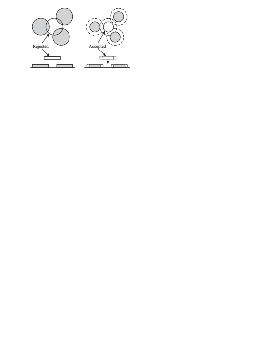
Figure 1: The left panel illustrates deposition attempts in 2D and 1D that are rejected due to particle overlap. The right panel shows a situation at a later time at which the same deposition attempts would succeed due to particle shrinkage.

 

The model is illustrated in Figure 1. We note that if the disks shrink too fast as compared to the time scale of the buildup of the deposited layer, which is of order $\sim 1/RD^{2}$, then the problem will be reduced to that of simply depositing smaller disks. On the other hand, if the disks shrink too slow as compared to the time scale $\sim 1/RD^{2}$, then the depletion of the correlations at contact will be trivially attributable to disk shrinkage alone. We are interested in the interplay of two effects: The decreasing disk size enlarges voids between already deposited disks. At the same time this process increases the rate of successful disk deposition events, which reduce voids between disks. Given that numerical simulations for this problem are quite demanding, we report results for the following time-dependence for the disk radius,

$$D(t)=D(\infty)\Big{\{}1+\exp[-RD^{2}(\infty)t]\Big{\}}\,.$$ (2)

We also studied numerically the cases

$$D(t)=D(\infty)\Big{\{}1+\frac{1}{\ln[e+RD^{2}(\infty)t]}\Big{\}}\,,$$ (3)

$$D(t)=D(\infty)\Big{\{}1+\frac{1}{1+RD^{2}(\infty)t}\Big{\}}\,,$$ (4)

and found qualitatively similar results.

II.2 Numerical results

Let us now briefly outline the numerical procedure used in our Monte Carlo simulations. In order to calculate the correlation function $P_{2}(r,t)$, we have to generate a distribution of deposited objects. We used periodic boundary conditions and system sizes $L\times L=500D(\infty)\times 500D(\infty)$. The $xy$-coordinates of the center of the next disc which makes a deposition attempt were randomly generated. If the disk does not overlap any of the previously deposited ones, then it is deposited. The total number of deposition attempts is thus equal to $RL^{2}\Delta t$ for a physical time interval $\Delta t$. All our data presented below, were averaged over 100 independent Monte Carlo runs.

We point out that there exist algorithms for studying RSA at large times Wang3 , specifically designed to account for the fact that isolated residual voids (defined as landing areas for particle centers for allowed depositions) then evolve independently. However, in our case we were primarily interested in intermediate times. Furthermore, as disks already adsorbed on the surface shrink, all the voids increase and some might merge to form larger voids. Therefore, we used the straightforward algorithm described in the preceding paragraph.

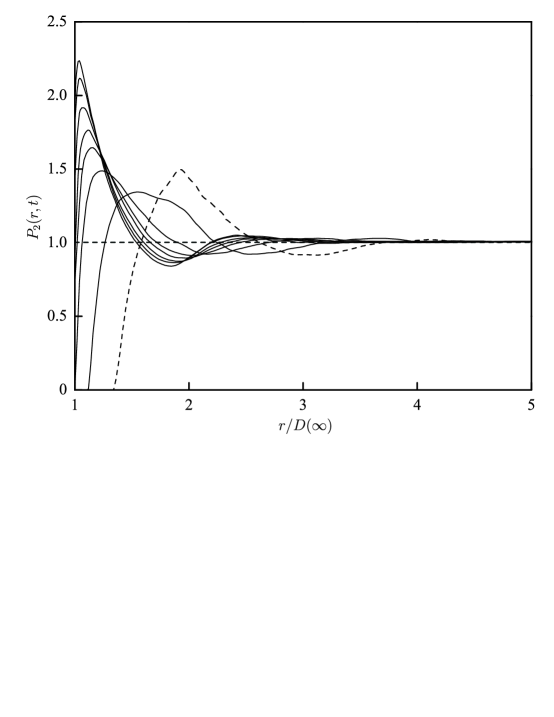
Figure 2: Time evolution of the correlation function in deposition of disks with diameters shrinking according to Eq. (2). The dashed line corresponds to $t=\tau$. The solid lines with increasing peak values at $r/D(\infty)$ approaching 1, correspond, respectively, to $t=2\tau$, $4\tau$, $6\tau$, $8\tau$, $12\tau$, $18\tau$, $24\tau$.

 

Our main result is illustrated in Figure 2. The correlation function introduced earlier, is plotted for several times, which are multiples of a characteristic process time-scale

$$\tau=1/RD^{2}(\infty)\,.$$ (5)

At finite times the correlation function has a peak at a value $r/D(\infty)>1$, and actually vanishes at the disk contact, when $r=D(t)$. This “correlation hole” behavior is in contrast with the ordinary RSA, e.g., Torquato1 , Feder , for which the correlation function instead of developing a peak close to contact, actually increases as the disk separation decreases towards contact, and reaches, for finite times, a constant, non-zero value at contact. The “correlation hole” property represents a formation of a certain degree of short-range ordering in the system, and specifically, avoidance of particle clumping.

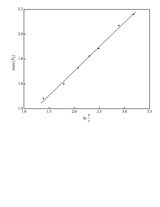
Figure 3: Time-dependence of the peak values of the correlation function, demonstrating the expected logarithmic divergence as $t\to\infty$. The least-squares fit of the peak values, shown here for times $t=4\tau$, $6\tau$, $8\tau$, $10\tau$, $12\tau$, $18\tau$, $24\tau$, yields the slope of the solid line as $0.37\pm 0.02$ (but note a comment in Subsection III.3 below regarding low reliability of this “error-bar” estimate).

 

In the limit $t\to\infty$, the correlation hole closes and the correlation function seems to develop a weak divergence as $r\to D(\infty)$. In fact, for constant disk diameters, this property has been studied by asymptotic analytical arguments Swendsen and numerically Torquato1 , Feder : The weak logarithmic divergence of the correlation function of RSA at contact, is not easy to quantify numerically, and our data were not accurate enough to study this limit for shrinking-diameter disk deposition by directly estimating $P_{2}(r,\infty)$. However, the time-dependence of the peak values in Figure 2, follows a logarithmic divergence as $t$ increases, as shown in Figure 3. This is reminiscent of a similar logarithmic divergence predicted Swendsen for the values of $P_{2}(D,t)$ at contact ($r=D$) for fixed-$D$ RSA.

Figure 4: The correlation function for $t=10\tau$, in deposition of disks with diameters shrinking according to Eq. (2): dashed line; Eq. (3): solid line; and Eq. (4): dotted line.

 

The formation of the finite-time correlation hole at disk-contact, was observed also for the non-exponential disk-diameter time-dependences defined in Eqs. (3-4); see Figure 4. This property of the correlation function is qualitatively similar for all three time-dependence protocols studied. However, we did not study larger time values for the non-exponential time-dependences.

III Deposition of Segments on a Line

III.1 Numerical results

In this section we report numerical results for the 1D deposition of segments on an initially empty line. The segment length is a function of time, $\ell(t)$, monotonically decreasing from $\ell(0)$ to $\ell(\infty)$. Our numerical results in 1D were obtained for the exponential time dependence similar to the 2D case,

$$\ell(t)=\ell(\infty)\Big{\{}1+\exp[-R\ell(\infty)t]\Big{\}}\,.$$ (6)

We denote the number of deposition attempts per unit time per unit length (the flux) by $R$. The arriving segments are adsorbed only if they do not overlap any previously deposited ones; see Figure 1. The quantity of interest is the gap density distribution function, $G(x,t)$: The density of gaps (measured between the ends of the nearest-neighbor deposited segments) of length between $x$ and $x+dx$ at time $t$ is $G(x,t)dx$. The density of deposited segments at time $t$, which in 1D equals the density of gaps, is given by

$$n(t)=\int^{\infty}_{0}G(x,t)dx\,.$$ (7)

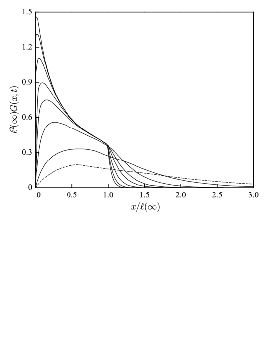
Figure 5: Time evolution of the dimensionless gap-size distribution function $\ell^{2}(\infty)G(x,t)$ for segments with length shrinking according to Eq. (6). The dashed line corresponds to $t=\tau$. The solid lines with increasing peak values at $x/\ell(\infty)$ eventually approaching 0, correspond, respectively, to $t=2\tau$, $4\tau$, $6\tau$, $8\tau$, $12\tau$, $18\tau$, $24\tau$.

 

Our numerical simulations followed the same procedure as in 2D. In 1D, we used periodic boundary conditions and system sizes $10000\ell(\infty)$. The time scale, cf. Eq. (5), was redefined for 1D,

$$\tau\equiv 1/R\ell(\infty)\,.$$ (8)

Our results, shown in Figure 5, represent averages over 10000 independent Monte Carlo runs. One can see that the gap density distribution function is a smooth function of $x$ for finite times, $t$, and for larger times it develops a pronounced peak at $x<\ell(t)$ approaching $x=0$. However, at $x=0$ for finite times there is a “correlation hole.” In the large-time limit, $G(x,t\to\infty)$ appears to develop a step at $x=\ell(\infty)$, as well as a divergence at $x=0$. These properties will be further discussed in the next two subsections.

III.2 Analytical considerations

In this subsection, we will consider an analytical kinetic equation approach to the 1D deposition problem. This will allow us to elucidate the origin of the “correlation hole” at $x=0$. Kinetic equations, closed-form or hierarchies of, for RSA can be formulated for the gap density distribution function as well as for several other correlation-function-type quantities. They have been widely used for deriving exact results and low-density approximation schemes; see reviews in Evans , Privman1 , Privman3 , Privman55 . For the present problem, we have

$$\frac{\partial G(x,t)}{\partial t}=-R\theta(x-\ell(t))[x-\ell(t)]G(x,t)+2R\int^{\infty}_{x+\ell(t)}G(y,t)dy+\dot{\ell}(t)\frac{\partial G(x,t)}{\partial x}\,.$$ (9)

Here the first term represents the destruction of gaps of length $x$ by segment deposition, with $\theta(\ldots)$ denoting the standard step function which vanishes for negative arguments and is 1 for positive arguments. The second term represents the creation of gaps of length $x$ due to deposition of segments landing in larger gaps of size $y>x+\ell(t)$. The last term describes the increasing size of all the gaps as a result of segment shrinkage. Note that the case $\dot{\ell}(t)=0$ is exactly solvable Gonzalez , and we will be using some of the exact results in the next subsection. For large $x$, we obviously have the boundary condition $G(x\to\infty,t>0)=0$ for Eq. (9). The following discussion explores the form of the boundary condition at the small-$x$ side of the distribution.

There are two kinetic processes that alter gap lengths in our problem. First, deposition of segments can reduce the length by $\ell(t)$. This process can generate very small, positive gap lengths, $\epsilon$, from available gaps of sizes $\ell(t)+\epsilon$. At the same time, the second process, that of segment shrinkage, causes all gap lengths to “drift” towards larger positive values with velocity $-\dot{\ell}(t)$. These two kinetic processes determine the evolution of the gap-length distribution $G(x,t)$ from its initial value $G(x,0)$. While our numerical simulations were for $G(x,0)=0$, we note that in principle one can generate other translationally invariant initial distributions by an appropriate preparation of the initial state. In fact, one can even prepare initial distributions that extend to small negative gap lengths. This entails allowing overlaps for the segments initially placed on the line, but not for those later depositing. If the segments are ordered according to their center-point positions, and each gap is measured as a consecutive center-point distance minus $\ell(t)$, then the initial-distribution overlaps, even if some are multi-segment, can be unambiguously counted as negative gaps. The two kinetic processes will then remain the same: Gaps larger than $\ell(t)$ can be shortened due to deposition events, while at the same time all the gaps (positive, zero, negative) also increase towards positive values, due to segment shrinkage.

The above considerations suggest that equation Eq. (9) strictly speaking should be mathematically considered for $-\infty<x<\infty$. An attempt to limit it to $0\leq x<\infty$, and also use moment definitions, such as the zeroth-order moment Eq. (7), with integration over $0\leq x<\infty$, may in general yield wrong results: Neglecting the “flow of length” from the negative-$x$ values may violate length conservation. However, in our case, specifically for the initial condition $G(x,0)=0$ (and with nonvanishing $\ell(t)$ for all $t$, including in the $t\to\infty$ limit, which avoids a possible singular limit), it is obvious that the problem should be definable with a boundary condition at $x=0$ because all the kinetics of the process occurs in $0\leq x<\infty$. Indeed, together with the zeroth-order moment, the first-order moment of the distribution can be used to determine the applicable boundary condition directly from length-conservation,

$$\ell(t)n(t)+\int_{0}^{\infty}xG(x,t)dx=1\,.$$ (10)

Here the first term is the density of the covered area, whereas the second term is the density of the uncovered area. Both densities are “per unit length” in 1D, and therefore they sum up to 1. Differentiation with respect to time, $t$, and the use of Eq. (9), then yield, after some algebra, the result

$$\dot{\ell}(t)G(0,t)=0\,.$$ (11)

For shrinking segments, $\dot{\ell}<0$, we are thus led to our main conclusion,

$$G(0,t)=0\,,$$ (12)

except perhaps in the limit $t\to\infty$ (in which $\dot{\ell}$ vanishes). This result indicates that the “correlation hole” for finite times, at $x=0$ is generic for the shrinking-segment RSA, no matter how fast is the deposition kinetics that tends to “fill the hole” in the distribution at small $x$: The presence of the correlation hole (the depletion of the gap-distribution near $x=0$) follows from the boundary condition established for $x=0$.

III.3 Properties of the gap-length distribution

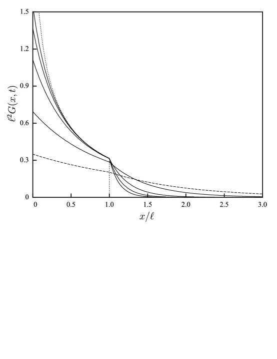
Figure 6: Time evolution of the dimensionless gap-size distribution function $\ell^{2}G(x,t)$ for segments of constant length $\ell$. The dashed line corresponds to $t=\tau$. The solid lines correspond to $t=2\tau$, $4\tau$, $6\tau$, $8\tau$, with increasing peak values at $x=0$, increasing values at $x=\ell$, and with respectively smaller values for $x\gg\ell$. The dotted line corresponds to $t\to\infty$, with the values for $x>\ell$ equal 0 in this limit.

 

For ordinary 1D RSA of segments of fixed length $\ell(t)=\ell\equiv\ell(\infty)$, Figure 6 illustrates the exact solution Gonzalez for several times and in the limit $t\to\infty$. Specifically, the gap distribution has a finite value at $x=0$, consistent with Eq. (11) for $\dot{\ell}=0$. This value actually diverges in the $t\to\infty$ limit, while a logarithmic singularity develops near $x=0$. This suggests that ordinary RSA is actually a rather singular limit of the more general shrinking-segment RSA. Indeed, the point $x=\ell(t)$ corresponds to discontinuity in the first, deposition term in the kinetic equation, Eq. (9). As a result, the fixed-$\ell$ RSA gap-distribution has a discontinuous derivative at $x=\ell$, which becomes an actual discontinuity (jump) in the $t\to\infty$ limit. On the other hand, with segment shrinking allowed the distribution is apparently continuous and smooth (as numerically observed), likely analytic at all points internal to the domain of definition, $0<x<\infty$, of the gap distribution. Adding the segment shrinkage process seems to smooth the singularities out for finite times; cf. Figure 5. In terms of the kinetic equation, this is a consequence of that the added third, $\sim\partial G/\partial x$ term plays the role of the “diffusive” (second-derivative) smoothing contribution with respect to the $x$-dependent integral (the second term). This diffusive property of the kinetic equation suggests that the function $G(x,t)$ has no singularities for any $x>0$ for finite time, though in the limit $t\to\infty$ (when $\dot{\ell}(t)\to 0$) the divergence as $x\to 0^{+}$ and the discontinuity at $x=\ell(\infty)$ are asymptotically restored.

The exact solution technique for the constant-length case Gonzalez involves the use of the exponential-in-$x$ ansatz for $G(x,t)$ for $x>\ell$, recently detailed in applications for related models in BN , Privman7 , and then solution of the $x<\ell$ equation, Eq. (9), which becomes tractable because the first term is not present, whereas the integration in the second term involves a simple exponential integrand. Thus, this approach by its nature yields discontinuities if not in the function then in its first or possibly higher-order derivatives. Attempts to use this approach, as well as more complicated, exponential-multiplied-by-polynomial ansaetze for $x>\ell(t)$, for time-dependent $\ell(t)$ yield solutions which satisfy the equation but possess unphysical discontinuities. We consider it unlikely that the shrinking-segment RSA problem in 1D can be solved exactly by the presently known techniques.

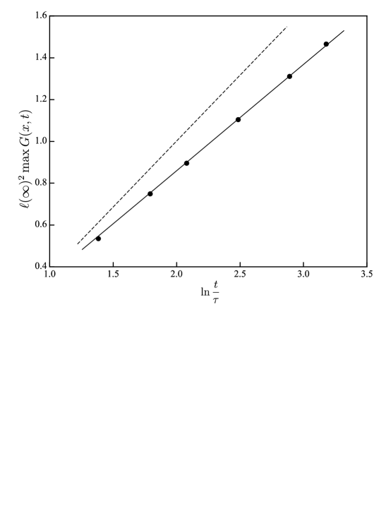
Figure 7: The dashed straight line is the asymptotic large-time form of the gap-distribution function for the fixed-segment-length RSA; its slope is $2e^{-2\gamma}$ see Eq. (13). The solid straight line is a fit of our data (shown as symbols) for $t\geq 4\tau$, for shrinking-segment RSA, with the estimated slope of $0.51\pm 0.02$.

 

Finally, let us consider the extent to which our numerical data can confirm the restoration of the logarithmic singularity near $x=0$ in the $t\to\infty$ limit. As in 2D, our data are not accurate enough to confirm the form of the $x$-dependence of the expected logarithmic divergence for $x\ll\ell(\infty)$, i.e., $G(x,\infty)\propto-\ln\left(x/\ell(\infty)\right)$. Regarding the $t$-dependence, Figure 7 shows our 1D data for the peak values at small positive $x$, see Figure 5, as well as the asymptotic large-time form of the exact solution peak values at $x=0$ for constant $\ell=\ell(\infty)$, the latter given by the relation Gonzalez

$$\ell^{2}G(t,0)\simeq 2e^{-2\gamma}\ln({t}/{\tau}),\qquad t\gg\tau\,,$$ (13)

where $\gamma=0.5772156649\ldots$ is Euler’s gamma constant. Typical for data fits for logarithmic dependences, the estimated slope given in Figure 7, may gradually drift as the $t$-variable varies over many decades. It is possible that it reaches the larger value of the fixed-segment RSA: We consider the error estimate, 0.02, here and in the 2D case (Figure 3) inconclusive.

In summary, we investigated an RSA model in which deposition of arriving objects, which tends to form small gaps/voids, competes with the process of shrinking of the objects, both those already deposited and those newly arriving. The latter process always “wins” at finite time, and as a result “correlation hole” opens up in the correlation properties considered. In fact, analytical considerations in 1D suggest that this property is generic for an initially empty substrate. Numerical Monte Carlo results reported, support this conclusion for the time-dependences studied. For the exponential-decay time dependence of the object sizes studied in 1D and 2D, we also found preliminary evidence that logarithmic divergence of the correlation properties at contact is restored as $t\to\infty$. For 1D, the discontinuous behavior of the gap-distribution at $x=\ell(\infty)$ also reemerges in this limit.

The authors thank Drs. S. Minko and I. Tokarev for instructive discussions, and acknowledge support of this research by the NSF under grant DMR-0509104.

References

- (1) Review: J. W. Evans, Rev. Mod. Phys. 65, 1281 (1993).
- (2) Review: M. C. Bartelt and V. Privman, Int. J. Mod. Phys. B 5, 2883 (1991).
- (3) Collection of review articles: Adhesion of Submicron Particles on Solid Surfaces, V. Privman, ed., special volume of Colloids and Surfaces A 165, Issues 1-3, Pages 1-428 (2000).
- (4) Collection of review articles: Nonequilibrium Statistical Mechanics in One Dimension, V. Privman, ed. (Cambridge University Press, Cambridge, 1997).
- (5) Review: J. J. Ramsden, Chem. Soc. Rev. 24, 73 (1995).
- (6) P. R. Van Tassel, P. Viot and G. Tarjus, J. Chem. Phys. 106, 761 (1997).
- (7) S. Torquato, O. U. Uche and F. H. Stillinger, Phys. Rev. E 74, 061308 (2006).
- (8) A. V. Subashiev and S. Luryi, Phys. Rev. E 75, 011123 (2007).
- (9) Review: V. Privman, J. Adhesion 74, 421 (2000).
- (10) W. van Roosbroeck, Phys. Rev. 139, A1702 (1965).
- (11) R. C. Alig, S. Bloom and C. W. Struck, Phys. Rev. B 22, 5565 (1980).
- (12) M. Inoue, Phys. Rev. B 25, 3856 (1982).
- (13) P. Viot, G. Tarjus and J. Talbot, Phys. Rev. E 48, 480 (1993).
- (14) J.-S. Wang, P. Nielaba and V. Privman, Physica A 199, 527-538 (1993).
- (15) D. Boyer, J. Talbot, G. Tarjus, P. Van Tassel and P. Viot, Phys. Rev. E 49, 5525 (1994).
- (16) Z. Adamczyk and P. Warszyński, Adv. Colloid Interf. Sci. 63, 41 (1996).
- (17) G. J. Rodgers and Z. Tavassoli, Phys. Lett. A 246, 252 (1998).
- (18) M. K. Hassan, J. Schmidt, B. Blasius and J. Kurths, Phys. Rev. E 65, 045103R (2002).
- (19) D. J. Burridge and Y. Mao, Phys. Rev. E 69, 037102 (2004).
- (20) N. A. M. Araújo and A. Cadilhe, Phys. Rev. E 73, 051602 (2006) .
- (21) P. Nielaba and V. Privman, Modern Phys. Lett. B 6, 533 (1992).
- (22) J.-S. Wang, P. Nielaba and V. Privman, Modern Phys. Lett. B 7, 189 (1993).
- (23) M. C. Bartelt and V. Privman, Phys. Rev. A 44, R2227 (1991).
- (24) A. Cadilhe, N. A. M. Araújo and V. Privman, J. Phys. Cond. Matter 19, 065124 (2007).
- (25) N. A. M. Araújo, A. Cadilhe and V. Privman, Phys. Rev. E 77, 031603 (2008).
- (26) V. Privman and P. Nielaba, Europhys. Lett. 18, 673 (1992).
- (27) E. Ben-Naim and P. L. Krapivsky, Phys. Rev. E 54, 3562 (1996).
- (28) O. Gromenko, V. Privman and M. L. Glasser, J. Comput. Theor. Nanosci., in print (2008).
- (29) V. Privman, Europhys. Lett. 23, 341 (1993).
- (30) N. V. Dziomkina and G. J. Vancso, Soft Matter 1, 265 (2005).
- (31) J. A. Liddle, Y. Cui and P. Alivisatos, J. Vac. Sci. Technol. B 22, 3409 (2004).
- (32) T. Ogawa, Y. Takahashi, H. Yang, K. Kimura, M. Sakurai and M. Takahashi, Nanotechnology 17, 5539 (2006).
- (33) R. D. Deshmukh, G. A. Buxton, N. Clarke and R. J. Composto, Macromolecules 40, 6316 (2007).
- (34) R. Lupitskyy, M. Motornov and S. Minko, Langmuir 24, 8976 (2008).
- (35) M. Motornov, R. Sheparovych, R. Lupitskyy, E. MacWilliams and S. Minko, J. Colloid Interf. Sci. 310, 481 (2007).
- (36) N. Nath and A. J. Chilkoti, J. Am. Chem. Soc. 123, 8197 (2001).
- (37) I. Tokareva, S. Minko, J. H. Fendler and E. Hutter, J. Am. Chem. Soc. 126, 15950 (2004).
- (38) Z. Y. Zhong, S. Patskovskyy, P. Bouvrette, J. H. T. Luong and A. Gedanken, J. Phys. Chem. B 108, 4046 (2004).
- (39) S. Lee and V. H. Pérez-Luna, Anal. Chem. 77, 7204 (2005).
- (40) I. Tokareva, I. Tokarev, S. Minko, E. Hutter and J. H. Fendler, Chem. Commun. 3343 (30 June 2006).
- (41) O. Azzaroni, A. A. Brown, N. Cheng, A. Wei, A. M. Jonas and W. T. S. Huck, J. Mater. Chem. 17, 3433 (2007).
- (42) Y. Ding, X. H. Xia and H. S. Zhai, Chem. Eur. J. 13, 4197 (2007).
- (43) Y. Pomeau, J. Phys. A 13, L193 (1980).
- (44) R. H. Swendsen, Phys. Rev. A 24, 504 (1981).
- (45) A. Yethiraj, C. K. Hall and K. G. Honnell, J. Chem. Phys. 93, 4453 (1990).
- (46) Y. C. Chiew, J. Chem. Phys. 93, 5067 (1990).
- (47) E. Kierlik and M. L. Rosinberg, J. Chem. Phys. 99, 3950 (1993).
- (48) J. Huh, O. Ikkala and G. ten Brinke, Macromol. 30, 1828 (1997).
- (49) V. Krakoviack, E. Kierlik, M.-L. Rosinberg and G. Tarjus, J. Chem. Phys. 115, 11289 (2001).
- (50) Strongly Coupled Coulomb Systems, G. J. Kalman, J. M. Rommel and K. Blagoev, eds. (Springer, New York, 2002).
- (51) J. Feder, J. Theor. Biol. 87, 237 (1980).
- (52) J.-S. Wang, Int. J. Mod. Phys. C 5, 707 (1994).
- (53) J. J. Gonzalez, P. C. Hemmer and J. S. Høye, Chem. Phys. 3, 288 (1974).