The Spine of the Cosmic Web

Abstract

We present the SpineWeb framework for the topological analysis of the Cosmic Web and the identification of its walls, filaments and cluster nodes. Based on the watershed segmentation of the cosmic density field, the SpineWeb method invokes the local adjacency properties of the boundaries between the watershed basins to trace the critical points in the density field and the separatrices defined by them. The separatrices are classified into walls and the spine, the network of filaments and nodes in the matter distribution. Testing the method with a heuristic Voronoi model yields outstanding results. Following the discussion of the test results, we apply the SpineWeb method to a set of cosmological N-body simulations. The latter illustrates the potential for studying the structure and dynamics of the Cosmic Web.

1. Introduction

The large scale distribution of matter revealed by galaxy surveys features a complex network of interconnected filamentary galaxy associations. This network, which has become known as the Cosmic Web (Bond et al., 1996), contains structures from a few megaparsecs up to tens and even hundreds of Megaparsecs of size. The weblike spatial arrangement of galaxies and mass into elongated filaments, sheetlike walls and dense compact clusters, the existence of large near-empty void regions and the hierarchical nature of this mass distribution – marked by substructure over a wide range of scales and densities – are its three major characteristics. Its appearance has been most dramatically illustrated by the recently produced maps of the nearby cosmos, the 2dFGRS, the SDSS and the 2MASS redshift surveys (e.g. Colless et al., 2003; Huchra et al., 2005).

In this paper we introduce the SpineWeb formalism for analyzing the structure and topology of the Cosmic Web. It identifies the sheets and filaments in the Cosmic Web, along with the large underdense void regions, and their mutual connection into the Spine of the cosmic matter distribution. The method is based on the Watershed Transform (WST, Beucher, 1982), and is largely free of user-specific parameters and artificial smoothing scale(s). Its output will enable the study of the physical properties and dynamics of the individual morphological components, along with their topology and hierarchical characteristics.

1.1. the Cosmic Web

The Cosmic Web is the most salient manifestation of the anisotropic nature of gravitational collapse, the motor behind the formation of structure in the cosmos (Peebles, 1980). N-body computer simulations have profusely illustrated how a primordial field of tiny Gaussian density perturbations transforms into a pronounced and intricate filigree of filamentary features, dented by dense compact clumps at the nodes of the network (Colberg, Krughoff & Connolly, 2005; Springel et al., 2005). The filaments connect into the cluster nodes and act as the transport channels along which matter flows into the clusters.

Fundamental understanding of anisotropic collapse on cosmological scales came with the seminal study by Zeldovich (1970), who recognized the key role of the large scale tidal force field in shaping the Cosmic Web (also see Icke, 1973). The collapse of a primordial cloud (dark) matter passes through successive stages, first assuming a flattened sheetlike configuration as it collapses along its shortest axis. This is followed by a rapid evolution towards an elongated filament as the intermediate axis collapses and, if collapse continues along the longest axis, may ultimately produce a dense, compact and virialized cluster or halo. The hierarchical setting of these processes, occurring simultaneously over a wide range of scales and modulated by the expansion of the Universe, complicates the picture considerably. Recent state-of-the-art computer experiments like the Millennium simulation (Springel et al., 2005) clearly show the hierarchical nature in which not only the clusters build up but also the filamentary network itself (see Aragón-Calvo et al., 2007b).

The Cosmic Web theory of Bond et al. (1996) succeeded in synthesizing all relevant aspects into a coherent dynamical and evolutionary framework. It is based on the realization that the outline of the cosmic web may already be recognized in the primordial density field. The statistics of the primordial tidal field explains why the large scale universe looks predominantly filamentary and why in overdense regions sheetlike membranes are only marginal features (Pogosyan et al., 1998). Of key importance is the observation that the rare high peaks, which will eventually emerge as clusters, are the dominant agents for generating the large scale tidal force field: it is the clusters which weave the cosmic tapestry of filaments (Bond et al., 1996; van de Weygaert & Bertschinger, 1996; van de Weygaert & Bond, 2008a). They cement the structural relations between the components of the Cosmic Web and themselves form the junctions at which filaments tie up. This relates the strength and prominence of the filamentary bridges to the proximity, mass, shape and mutual orientation of the generating cluster peaks: the strongest bridges are those between the richest clusters that stand closely together and point into each other’s direction.

The emerging picture is one of a primordially and hierarchically defined network whose weblike topology is imprinted over a wide spectrum of scales. Weblike patterns on ever larger scales get to dominate the density field as cosmic evolution proceeds, and as small scale structures merge into larger ones. Within the gradually emptying void regions, however, the topological outline of the early weblike patterns remains largely visible.

1.2. Closing in on the Cosmic Web

Despite a large variety of attempts, as yet no generally accepted descriptive framework has emerged for the objective and quantitative analysis of the geometry and topology of the Cosmic Web. The great complexity of both the individual structures as well as their connectivity, the lack of structural symmetries, its intrinsic multiscale nature and the wide range of densities that one finds in the cosmic matter distribution has prevented the use of simple and straightforward techniques.

Historically, the quantitative analysis of the Cosmic Web has been dominated by a description in terms of statistical measures of clustering of galaxies and matter. While correlation functions have been the mainstay of the cosmological analysis of large scale structure, a direct interpretation in terms of the patterns and texture of the Cosmic web has largely remained elusive. Over the years a variety of heuristic measures have been forwarded to analyze specific aspects of the spatial patterns in the large scale Universe, but only in recent years there have been attempts towards developing complete descriptors of the intricate spatial patterns that define the Cosmic Web. Nearly without exception these methods borrow extensively from other branches of science such as image processing, mathematical morphology, computational geometry and medical imaging.

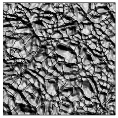
Figure 1.— Top left: a slice of 100 $h^{-1}$ Mpc of side showing the density field computed from a N-body simulation. Top right: the same slice as the left panel but here showing the density field as a shaded landscape where high density regions correspond to ridges while underdense regions correspond to valleys. The light source used to shade the surface is located at the north-east. Bottom left: the 2D watershed transform computed from the 2D density field using a discrete-intensity bucket algorithm (black contours). Each individual valley is randomly colored for visualization purposes. Bottom right: the same landscape as the top right panel but here we also show the watershed transform superimposed as thick black lines. The watershed contour has been slightly smoothed for visualization purposes.

Noteworthy examples include filament detection with the help of the Candy model (Stoica et al., 2005) and wavelet analysis of the Cosmic Web (Martínez et al., 2005). Several methods seek to relate morphological features to singularities in the density field, usually invoking information on the gradient and Hessian of the density field, or of the tidal field (see e.g. Sousbie et al., 2008a; Aragón-Calvo et al., 2007a, b; Hahn et al., 2007a, b; Bond et al., 2009). A classification scheme on the basis of the manifolds in the tidal field – involving all morphological features in the cosmic matter distribution – has been presented by Hahn et al. (2007a, b); Forero-Romero et al. (2008). However, its success may depend strongly on the correct choice of the smoothing scale. Another concept addressing the gradient and Hessian of the density field is that of the skeleton analysis, a direct application of Morse theory to cosmological density fields (see Colombi et al., 2000; Pogosyan et al., 2009). The skeleton formalism has been developed for the morphological analysis of the Megaparsec Cosmic Web, in redshift surveys like SDSS as well as in N-body simulations (Novikov et al., 2006; Sousbie et al., 2008a, b, 2009). Its present implementation refers to features identified at one single specific scale and suffers from Gaussian smoothing. The multiscale nature of the cosmic matter distribution is explicitly addressed by the Multiscale Morphology Filter, which is based on a scale-space analysis of the Hessian of the density field Aragón-Calvo et al. (2007a, b) to identify cluster, filaments and sheets on the scale where they are locally most prominent.

1.3. Watershed and Cosmic Spine

One technique that implicitly addresses the topology of the Cosmic Web is the Watershed Void Finder (WVF) developed by Platen et al. (2007). The WVF is an application of the Watershed Transform for the identification of underdense basins in the megaparsec-scale matter distribution. The Watershed transforms segments the density field into isolated basins and delineates the boundaries of cosmological voids.

The method presented in this paper is the natural extension of the Watershed Void Finder. It includes the watershed transform into a wider context as a framework for studying both the morphology and topology of the cosmic web and its various constituents. The result is the SpineWeb method, a complete framework for the identification of voids, walls and filaments. Via the practical role of the watershed transform in computing the Morse complex it is intimately related to Morse theory, in which it finds its mathematical foundation. It is important to note that although Morse theory can be used to describe the same topology traced by the SpineWeb method there is not a univocal relation between the two as the SpineWeb is based on the observed properties of the Cosmic Web.

An important aspect of our method is that it is an intrinsically scale-free method, starting from a scale-free reconstruction of the density field. We use the DTFE method of Schaap & van de Weygaert (2000), which guarantees an optimal and unbiased representation of the hierarchical nature and anisotropic morphology of cosmic structure (see van de Weygaert & Schaap, 2009, for an extensive description). Having guaranteed the capability of invoking a full scale-free Scale-space representation of cosmic structure, our watershed procedure not only traces the outline of filaments and sheets, but may also be extended towards doing so over a range of scales in order to address their hierarchical structure.

1.4. Outline

The principal rationale behind the SpineWeb analysis of the cosmic matter distribution is the interest in relating the geometry of the matter and galaxy distribution in a more meaningful fashion to the underlying dynamical evolution. One particular aspect of this dynamically motivated disentanglement of structure is the attempt to identify various evolutionary stages of the tidally induced anisotropic collapse of structure in the Universe.

In this paper we will focus specifically on the description of the basic SpineWeb formalism, confined to a density field sampled on a regular grid. We start by discussing the topological background of our study in section 2, focusing on the watershed transform, its connection to the general context of Morse theory and the related issues of practical interest to the SpineWeb formalism. The overall cosmological background of the structure, formation and dynamics of the Cosmic Web follows in section 3, amongst others to establish the link between the structures identified by the SpineWeb technique and the filamentary identity of tidal bridges in the theory of the Cosmic Web (Zeldovich, 1970; Bond et al., 1996). The technical aspects of the SpineWeb formalism are outlined in some detail in section 4. Subsequently, the formalism is tested by applying it to two different classes of spatial particle distributions. The first testbed concerns two simple heuristic Voronoi clustering models which model aspects of cellular and/or weblike spatial distributions. Visual and quantitative tests are described in section 5. The operation of SpineWeb in a more realistic setting of a $\Lambda$CDM simulation is the subject of section 6. In this section we also stress the fundamental differences between a structural selection based on density thresholds or one based on topological criteria. To illustrate the potential for analyzing cosmological structures, in section 7 we shortly describe three quantitative measures for the matter distribution in the $\Lambda$CDM simulation we used for testing. Finally, section 8 summarizes our results, and discusses prospects and further developments of the SpineWeb formalism.

2. Watershed Segmentation of the Cosmic Web

When studying the topological and morphological structure of the cosmic matter distribution in the Cosmic Web, it is convenient to draw the analogy with a landscape (see fig. 1, top row). Valleys represent the large underdense voids that define the cells of the Cosmic Web. Their boundaries are sheets and ridges, defining the network of walls, filaments and clusters that defines the Cosmic Web (cf. top panels fig. 1).

2.1. the Watershed Transform

The watershed transform (WST) is one of the most common methods used in Image analysis for segmenting images into distinct patches and features. It is a concept defined within the context of mathematical morphology, and was first introduced by Beucher & Lantuejoul (1979). The basic idea behind the WST stems from geophysics, where it is used to delineate the boundaries of separate domains, i.e. basins into which yields of e.g. rainfall will collect. The watershed transform is formed by the ridges and sheets surrounding the watershed basins and includes a subset of all the critical points in the density field.

The word watershed finds its origin in the analogy of the procedure with that of a landscape being flooded by a rising level of water. Suppose we have a surface in the shape of a landscape (cf. top right panel, fig. 1). The surface is pierced at the location of each of the minima. As the water-level rises a growing fraction of the landscape will be flooded by the water in the expanding basins. Ultimately basins will meet at the ridges defined by saddle-points and maxima in the density field. The final result of the completely immersed landscape is a division of the landscape into individual cells, separated by ridge dams (see left bottom panel fig. 1).

2.2. A watershed search for voids

The watershed transform was first introduced in a cosmological context as an objective technique to identify and outline voids in the cosmic matter and galaxy distribution (Platen et al., 2007; Platen, 2009). Following the density field-landscape analogy, the Watershed Void Finder (WVF) method identifies the underdense void patches in the cosmic matter distribution with the watershed basins. The method is parameter free in case there is no noise in the data.

A major advantage of the WVF method is its independence of assumptions on the shape and size of voids (see (Colberg et al., 2008) for a comparison of its performance with a variety of void finding algorithms). Sharing this virtue with a similar tessellation-based void finding method, ZOBOV (Neyrinck, 2008), WVF is particularly suited for the analysis of the hierarchical void distribution expected in the commonly accepted cosmological scenarios.

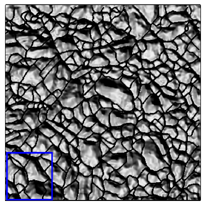
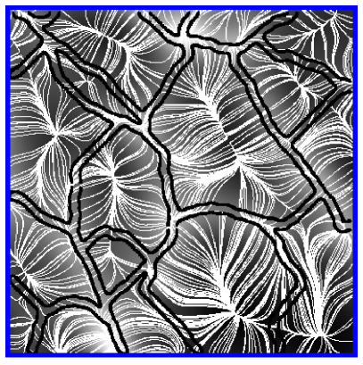
Figure 2.— Left: A slice of the density field shown as a shaded landscape with the watershed lines superimposed as black lines. Right: The zoomed area in the blue square of the left panel showing the slope lines (white lines) superimposed on the density field (gray background). The contour of the watershed transform is delineated by the thick black lines.

2.3. Watersheds and Landscape Gradients

Extrapolating its application to other areas of interest, the implementation of the watershed transform may also be seen as a practical instrument for the segmentation of surfaces and volumes on the basis of the topological structure of the “landscape” $f({\bf x})$. To trace the topological structure of a field $f({\bf x})$, we need to investigate the structure of the gradient field of the landscape, $\nabla f$ (for an excellent introduction to computational topology, we refer to Edelsbrunner (2010)).

2.3.1 Gradient Field and Integral Lines

The gradient delineates a smooth vector field, which vanishes at critical points,

$$\nabla f({\bf x_{k}})\,=0\,,$$ (1)

The integral lines or slope lines represent the flow along the gradient field $\nabla f$ between the critical points. On the basis of these connections one may infer a variety of spatial segmentations (see e.g. Cayley, 1859; Maxwell, 1870; Eberly, 1994; Furst, 2002; Edelsbrunner et al., 2003a, b; Danovaro et al., 2003; Gyulassy et al., 2005). One particular segmentation is the watershed transform, which segments the landscape $f$ into regions of uniform local gradient behavior: the watershed basin $j$ consists of the collection of points ${\bf x}$ that are closer in topographic distance $\mathcal{T}({\bf x},{\bf y}_{j})$,

$$\mathcal{T}({\bf x},{\bf y}_{j})\,\equiv\,{\rm inf}\int_{\Gamma}|\nabla f(\gamma(s))|ds\,.$$ (2)

to the defining minimum ${\bf y}_{j}$ of the basin than to any of the other minima. In this definition the integral is the pathlength along the integral line, the line along whose path the tangent at each point is parallel to the local gradient $\nabla f$. The watershed itself then consists of the ridge lines that delimit the boundaries between basins in the terrain.

An illustration of the close link between the gradient field and structural features in the Universe is offered by the righthand panel of fig. 2. The image shows that the integral lines that define the boundaries of adjacent valleys are in fact the watersheds. It also reveals the intimate relationship between the critical points in the flow field and the nodes, filaments and voids in the landscape: maxima are found at nodes of the weblike network of watershed ridges, minima at the centers of the void cells, while saddle points are to be found at key locations along the ridges. Following this view, we see that the watershed lines are the set of slope lines emanating from saddle points and connecting to a local maximum or minimum. Within this framework, saddle points have the crucial function of defining the sheets and filaments in the density field through their connection to the maxima via the integral lines.

Note that because the image in fig. 2 is a slice through a three-dimensional field, the identification between the structural elements and the critical points in the image is not entirely unequivocal (see below). Nonetheless, the principal observation is that the resulting weblike segmentation of space, and the corresponding boundary manifolds, contain the full information on its topological structure marked by sheets, filaments and nodes.

2.4. Morse theory

The vast majority of applications of the watershed transform concern the interior of the segmented regions. However, it is straightforward to extend its focus to other morphological components of the Cosmic Web, towards the delineation of the network of overdense ridges and walls which form the boundary manifolds of the cosmic density landscape.

This can be directly appreciated by noting the close relation between the definition of the watershed transform and the more formal concept of the Morse complex. Morse theory is the mathematical framework for the analysis of the topological structure of manifolds, by relating it to smooth, C²-differentiable, functions defined on those spaces. Central to Morse theory are the location and nature of the critical points – minima, maxima and saddle points – and their mutual connection via the gradient-based integral lines. These determine the morphological features of the functional surface.

Even though there are some differences between the two (see e.g. Gyulassy, 2008), the close similarity between the definition of the watershed transform and the concepts of Morse theory indicates that the computation of the watershed transform may be used as an efficient means of computing the various structural elements in a landscape dissected along the lines of Morse theory (Morse, 1934; Milnor, 1965).

In a cosmological context, the skeleton formalism (Novikov et al., 2006; Sousbie et al., 2008a, b, 2009) is also based on Morse theoretical concepts, via the gradient and/or Hessian of the density field. The approach followed in our SpineWeb procedure involves the specific application of the watershed transform for the analysis and description of the topology of the Megaparsec Universe, following our introduction of the concept in the context of cosmic density field analysis (Platen et al., 2007). Implicitly, this results in a pseudo-Morse segmentation (see e.g. Gyulassy, 2008; Edelsbrunner, 2010), with the advantage of opening the path towards a fully hierarchical formalism. This intimate relationship was also recognized by Sousbie et al. (2009), who used a probabilistic extension of the watershed technique in the latest version of the skeleton formalism.

2.5. The Discrete Watershed Transform

The implementation of the watershed transform in a large variety of scientific applications has to address a few important practical issues. A typical characteristic of most scientific images is their discrete nature.

The discreteness concerns two aspects: the spatial discreteness, ie. the discrete number of intervals at which the image has been sampled (pixels/voxels), and the discrete intensity levels at which the image has been sampled.

Image discreteness creates a few complications for an accurate calculation of the watershed transform. It renders it difficult to identify the existence and exact location of saddle points on the basis of a discretized local neighborhood. For the same reason, it is difficult to accurately extract slope lines.

Several methods for the extraction of critical points have been developed in an attempt to alleviate the limitations imposed by the discreteness of images. Among these, the discrete watershed transform algorithm (Beucher, 1982) represents a simple and elegant formalism for identifying the watershed separatrices and can be shown to converge to the continuous case (Najman & Schmitt, 1994). The procedure emulates the flooding of valleys or catchment basins in a (discrete) image representing a landscape. The points where two or more lakes converge are marked, and the algorithm continues until all the pixels in the image have been flooded. At the end of the process the image will be segmented into individual regions sharing a local minima, with the points that were marked as the dividing boundaries between two or more valleys defining the watershed transform.

A major asset of the intensity discretization is that it helps to remove faint features, and therefore also removes artefacts without the need of pre- or post-processing. Perhaps the greatest advantage is that discrete images allow the use of highly efficient algorithms but in general their use is limited to image segmentation since they give incorrect topologies.

In the case of images with continuous (floating point) values one retains the option of computing the watershed transform directly from the continuous intensity image, in addition to the option of discretizising the intensity. On the basis of the continuous image, the watershed transform would delineate the topology more accurately than would be feasible on the basis of the the discrete-level representation. However, it would involve a substantial increase in computational cost and of complexity of the code.

3. Spine of the Cosmic Web

The analogy between the watershed transform defining the boundary between underdense basins and the topology of the cosmic matter distribution is in itself one of the major justifications of the SpineWeb method presented in this study. Basic is the connection between the elements that form the Spine of the Cosmic Web: walls, filaments, clusters and voids.

1. The Cosmic Web is an interconnected system of dense compact clusters, elongated filaments and tenuous sheetlike walls. Visible through the galaxies, gas and dark matter populating these structural features, the Cosmic Web theory (Bond et al., 1996) teaches us that its topological outline was already present in the primordial perturbation field out of which all structure arose.

2. All of the elements of the Cosmic Web are interconnected. This is a crucial observation, which can be most readily appreciated by studying high resolution N-body simulations (e.g. Springel et al., 2005). Otherwise seemingly isolated objects usually turn out to be connected to less massive structures which become visible when assessing the mass distribution at a higher mass resolution. A tantalizing idea is that the galaxies found at the center of voids lie at the intersection of tenuous intra-void dark-matter filaments.(Zitrin & Brosch, 2009; Park & Lee, 2009; Stanonik et al., 2010).

3. Filaments are suspended between clusters or, dependent on scale, massive halo clumps. Their prominence and density may vary substantially, dependent on the mass, distance and alignment of the generating dark matter halos. However, the sheer presence of two matter clumps is already sufficient for the corresponding tidal force field to guarantee the topological presence of a filamentary bridge. Tenuous membranes permeate the space between adjacent filaments, and are part of the large wall which defines the boundary between two underdense voids. The wall boundary is outlined by various filaments, connecting each other at the cluster nodes.

Following these observations, the Cosmic Spine is defined as the topological network of nodes, filaments and sheets along which the cosmic matter distribution on large Megaparsec scales has assembled (see fig. 1).

4. The Spineweb Procedure

The key aspect of the SpineWeb procedure is that it exploits the intrinsic topological information contained in the Watershed Transform to delineate the Cosmic Spine. For the computation of the Cosmic Spine by means of the Watershed Transform it is necessary to address a few issues of practical importance.

4.1. Density field

In our current implementations of the SpineWeb procedure, we apply the DTFE method to reconstruct the density field from the spatial particle distribution.

The DTFE procedure produces a self-adaptive volume-filling density field on the basis of the Delaunay tessellation of the point distribution(Schaap & van de Weygaert, 2000; Schaap, 2007). DTFE density (and velocity) fields have been found to optimally trace a hierarchical matter distribution at any resolution level represented by the point sample, while at the same time resolving the local anisotropies in the matter distribution. This high level of sensitivity to the topology of the matter distribution, makes DTFE ideally suited for the SpineWeb procedure (for an extensive description of the DTFE procedure, see van de Weygaert & Schaap, 2009).

Given a spatial distribution of points, DTFE is based on the assumption that the density at the position of each point is proportional to the inverse of the total volume of the adjacent Delaunay tetrahedra, ie. to the volume of its contiguous Voronoi cell. Subsequently, the density field values at any location throughout the sample volume is determined by means of linear interpolation within the Delaunay tetrahedra of the corresponding Delaunay tessellation. Because a singular density determination at the central location of a voxel tends to introduce aliasing artefacts at high densities, we follow a slightly elaborate procedure. The density at each voxel of the “image” grid is determined on the basis of the DTFE density field sampled on a subgrid with a three times higher resolution and the density at each gridpoint set equal to the mean of the DTFE values at the 27 subgrid locations within the corresponding voxel.

In the applications described in this study, we compute the density field values at the voxels of a regular cubic grid. We use a fast and efficient implementation of the DTFE algorithm based on the publicly available CGAL library.

4.2. Watershed Implementation

The discrete watershed transform code we use in the SpineWeb procedure is an adaptation of the immersion and the topographical distance algorithms for floating point intensity values (see Roerdink & Meijster, 2000, for a review). The code assumes a density map which is sampled on a regular grid. Our C code computes the watershed transform from a double-precision $512^{3}$ grid in just a couple of minutes on a regular linux workstation.

In a first step, the code starts by finding and labeling the local minima in the density map, by identifying the voxels with the lowest density value among all their 26 neighbors. These local minima are the seeds of the void valleys to be identified by the watershed transform.

In a second step, we follow the topographical distance algorithm in order to obtain a fast segmentation of the space into locally connected underdense regions. For each voxel we identify the voxel among its 26 neighbors which has the lowest density. The maximum gradient paths are traced by iteratively connecting the voxels to their lowest density neighbor until the path reaches a local minimum. Subsequently, we assign the label of the corresponding minimum to the path.

In the third step we extract the watershed transform itself, ie. the boundaries between the void regions. The pixels in the watershed transform are identified by means of a local immersion algorithm. First, we identify all the voxels that lie at the boundaries between two or more regions. Subsequently, this subset of voxels is sorted in density and the standard immersion algorithm is applied. By following this two-step procedure, we avoid what would be the most expensive component of the algorithm. Instead of having to sort the complete density field, the sorting evaluations are restricted to the points in the watershed boundaries, a minor fraction of the complete volume.

In a final step, each of the pixels in the watershed boundary is assigned a morphological label, following its identification as void, wall or filament element, according to the criterion expressed in equation 3 and as illustrated in fig. 3.

While the watershed transform provides us with a highly efficient means of segmenting space into topologically well-defined elements, in general the watershed algorithm tends to overdo the segmentation, creating too many regions and identifying small noise in the image rather than real features (see Edelsbrunner, 2010). We circumvent this circumstance by preprocessing the density or distance field via a Gaussian smoothing of $\sigma=2$ voxels.

4.3. from Watershed to SpineWeb

From the analogy between the Cosmic Web and the watershed transform one can define, on the basis of the discrete watershed transform of a cosmic density field, a set of unique criteria to identify voids, walls and filaments.

The criteria are based on the properties of the local neighborhood of all the points that comprise the discrete watershed transform. Instead of computing at any given point the local eigenvalues of the Hessian of the density field, one may simply resort to the entirely equivalent evaluation of the identity of the surrounding 26 neighbor pixels (for the three-dimensional situation). By counting the number $\mathcal{N}_{\textrm{\tiny{voids}}}$ of adjacent watershed basins (voids) amongst these, it is straightforward to discriminate between voxels which belong to a void, a wall or a filament by means of the following set of rules:

$$\mathcal{N}_{\textrm{\tiny{voids}}}\qquad\left\{\begin{array}[]{rl}\quad=\;\;\;1,&\text{void}\\ \quad=\;\;\;2,&\text{wall}\\ \quad\geq\;\;\;3,&\text{spine}\\ &\text{(filament+clusters)}\\ \end{array}\right.$$ (3)

Note that in the present implementation we do not discriminate between filament or cluster node, and instead consider them to be part of the same spinal structure. In a future implementation we will include a density maximum criterion which would allow us to find the cluster nodes amongst the spine voxels. In addition we can easily identify regions in clusters by using one of the common halo finders available like friends of friends and isolate them from the identified filaments.

Our Spineweb technique exploits a purely local criterion for identifying the morphological nature of boundary pixels in the density field: it utilizes the full geometric structure of the watershed transform to limit the evaluation to the direct neighbours of each point. This differs from the implementation followed by Sousbie et al. (2009) who included a probability propagation scheme in the watershed flooding procedure from where the different elements of their skeleton were determined by finding their intersections between the corresponding peak and void patches.

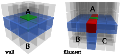
Figure 3.— Local neighborhood around a voxel (green) inside a wall (left) and filament (right). The blue voxels indicate walls and the red voxels filaments. The light gray cubes here represent voxels inside voids. The voxel inside a wall has two adjacent voids inside its neighborhood (A and B) while the voxel inside a filament has in this case three adjacent voids (A, B and C).

The above criterion is a purely and solely a topological one. By definition, walls are the regions between two adjacent voids. Filaments are to be found at the intersection of three watershed basins, at the intersection of 3 walls (see fig. 3). The success of these criteria can be appreciated from the 3-D surface maps in fig. 9 and the comparison between density and spine maps in fig. 10.

4.4. Image Grid Representation

While a regular grid facilitates the computation of the watershed transform and the subsequent topological identification of the various boundary pixels (see fig. 3), its simplicity may also involve a few possibly artefacts.

The first artefact relates to the discrete nature of the voxels in the density field. As a results, the filaments and walls have an artificial thickness - even if they would be infinitesimally thin - which makes the look pixelated or jagged. A particularly good illustration of this is the Spine obtained for the Voronoi clustering model in fig. 5 (panel c) where we explicitly render individual voxels as cubes. In the asymptotic limit of infinitesimally thin voxels the discrete watershed will converge to the continuous case.

The second artefact concerns the anisotropic nature of the local neighborhood of each voxel: Each voxel has 6 neighboring voxels at a distance $d=1$ (in voxel units), 16 neighbors at $d=\sqrt{2}$ and 8 neighbors at $d=\sqrt{3}$. it also involves an angular neighbor distribution deviating substantially from angular isotropy. A possible alternative would be to limit the neighborhood evaluation to the 6 most direct neighbors. However, the poor sampling might lead to a considerable risk of missing important topological information. For two-dimensional images the solution would be more straightforward. The use of a hexagonal grid would involve equal distance for all neighbor pairs and a perfectly uniform angular distribution. Unfortunately, an equivalent perfect grid for the three-dimensional situation does not exist. However, the use of Centroid Voronoi Tessellations (CVT, Du et al. (1999)) would certainly help to alleviate the main artefacts.

4.5. Galaxy Spine Assignment

Physically, filaments and walls are not infinitesimally thin structures. To identify the particles or galaxies attached to them, we therefore need to the define a (natural) thickness which encloses these objects.

In the applications described below, we account for this by applying the dilation morphological operator to the voxels labeled as filament and wall. The process increases the thickness of filaments and walls by one voxel and this procedure can be performed iteratively to further increase the thickness. The dilation operator was applied first to voxels labeled as wall and subsequently to pixels labeled as filaments following the number of degrees of freedom in the local variation of the density field, i.e. first walls and subsequently filaments (Aragón-Calvo et al., 2007b). In our particular case a single iteration with a $3\times 3\times 3$ kernel provides a good result without excessively fattening the structures.

5. SpineWeb Test:
    Voronoi Clustering models

To test and quantify in an objective way the identification of walls and filaments with the SpineWeb procedure we apply it to a few realizations of Voronoi Clustering models of the large scale matter distribution (van de Weygaert & Icke, 1989; van de Weygaert, 2002, 2010).

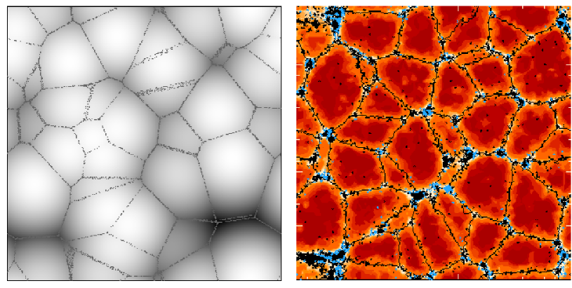
Figure 4.— Left: slice of the distance field computed from the Voronoi seeds (background). The particles located inside filaments, walls and nodes are also shown. Right: Voronoi model with density field reconstruction. A slice across the intensity of the density field is shown in orange scale in the background. The black lines correspond to the watershed transform and the particles are indicated by small diamonds. Blue particles are misclassifications (in all the categories) black particles are correct classified particles.

The Voronoi clustering models are heuristic models for cellular spatial patterns which use the geometric (and convex) structure of the Voronoi tessellation (Voronoi, 1908; Okabe, 2000) to emulate the cosmic matter distribution. They offer flexible templates for cellular patterns and are easy to tune towards a specific spatial cellular morphology. This makes them very suited for studying clustering properties of nontrivial geometric spatial patterns. Because the location, geometry and identity of the various spatial components in Voronoi models are known precisely, they are ideal as testbeds for the SpineWeb procedure. Unless otherwise specified, the seeds of the tessellation usually involve a set of Poisson distributed pints.

The Voronoi models use the corresponding tessellation for defining the structural frame around which matter will gradually assemble during the formation and growth of cosmic structure. Points are distributed within this framework by assigning them to one of the four distinct structural components of a Voronoi tessellation:

1. Void:
   regions located in the interior of Voronoi cells.

2. Wall:
   regions within and around the Voronoi cell faces.

3. Filament:
   regions within and around the Voronoi cell edges.

4. Clusters:
   regions within and around the Voronoi cell vertices.

What is usually described as a flattened “supercluster” consists of an assembly of various connecting walls in the Voronoi foam, while elongated “superclusters” of “filaments” usually include a few coupled edges. Vertices are the most outstanding structural elements, corresponding to the very dense compact nodes within the cosmic web where one finds the rich clusters of galaxies.

Among a variety of possible Voronoi clustering realizations, two distinct yet complementary classes of models are the most frequently used ones, the structurally rigid Voronoi Element Models and the evolving kinematic Voronoi models (see e.g. van de Weygaert, 2010, for an extensive description). Here we use one Voronoi Element Model, a composite of all four distinct components, and one realization of a Voronoi kinematic model.

In the case of the Voronoi Element model, the walls, edges and vertices are infinitely thin, yielding a pure geometric discrete realization of the underlying Voronoi tessellation. The Voronoi kinematic model represents a more realistic situation in which the various structures are assigned a finite width. We first analyze the topologically cleaner configuration of the Voronoi Element model, to assess the performance of SpineWeb under optimal conditions. Subsequently, we investigate whether in how far it can sustain this performance under less optimal circumstances.

5.1. Voronoi Element model

Based on a uniform distribution of $M$ cell seeds in a (periodic) box of size L, we start with a uniform distribution of N particles throughout a (periodic) box of size L. The particles are distributed within the tessellation by projecting them - with respect to the seed of the cell in which they are originally located - onto the walls, edges or vertices surrounding their Voronoi cell. As a result each of the walls, filaments and vertices have a different density, although the density remains uniform within each of the individual elements.

The Voronoi Element models we used for our test consisted of a set of particles distributed in a box of size L with $10^{6}$ particles from which $70\%$ resides in the walls, $25\%$ in the filaments and $5\%$ in the clusters. We chose a realization completely devoid of particles in the interior of voids. This distribution of particles was chosen in order to obtain a more uniform sampling over the three morphologies compared to a more realistic distribution.

5.1.1 Voronoi Distance Field

For the purpose of this test, instead of basing the SpineWeb procedure on the reconstructed (and noisy) density field we use the knowledge of the underlying tessellation to define a clean distance field.

The main idea behind the SpineWeb method, the identification of morphological structures on the basis of their topology, does not depend on practical details of the density field determination from a dataset of observed galaxy locations or computer simulations. In this respect, it is important to realize that the validity of the SpineWeb procedure can be tested and assessed on the basis of the topological structure of any field that is topologically equivalent to the density field of the Cosmic Web. This indeed is true for the distance field, and any generic field marked by a monotonic increasing value from a field minimum towards its watershed transform.

In the particular implementation described in this section, the distance field is defined as the Euclidean distance from each particle to its closest Voronoi seed. Regions close to the cell centers have low values while regions in the planes and edges of the cell have large values, with the value gradually increasing along the direction from the Voronoi cell centers towards the projected location on the walls. Within the walls, the highest density is reached at the surrounding edges, ultimately peaking at the vertices. In the resulting distance field, small cells correspond to low field values, while the larger cells yield higher field values, particularly near their boundaries. Following this definition, the distance field emulates the range of densities encountered in the Cosmic Web. The finite volumes of Voronoi cells in periodic tessellations assures a convergence of the distance field on the boundaries of data volume.

Various definitions of distance fields might be used, largely dictated by the specific questions at hand. An example of one such possibility would be to normalize the distance field on the basis of the distance to of the point to its second closest Voronoi nucleus, or the distance of its projected location on the corresponding Voronoi wall. The resulting distance field would reach a value of unity at the walls of the Voronoi cells. However, we opted to use the distance field with no normalization since it gives a better representation of the large dynamical range of densities encountered in the Cosmic Web.

5.1.2 Distance Field Realization

For the Voronoi Element test model, we determined the distance field on a cubic $512^{3}$ grid. For each of the pixels in the grid we identify the closest nucleus, among the set of $M$ generating nuclei. The pixel is assigned the value of its Euclidean distance.

The resulting field is shown in fig. 4. It depicts the distance field itself, in a planar section through the 3-D box, by means of a greyscale map. The corresponding particles located in the filaments, walls and nodes, within a narrow strip around the sectional plane, are superimposed on the image.

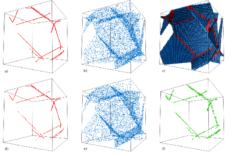
Figure 5.— The SpineWeb method applied to a Voronoi distribution. a) original particles lying at the edges of the Voronoi cells (filaments). b) original particles lying at the faces of the Voronoi cells (walls). c) Pixels inside filaments (red) and walls (blue) identified with the SpineWeb method. d) recovered particles lying at the edges of the Voronoi cells (filaments). e) recovered particles lying at the faces of the Voronoi cells (walls). f) particles erroneously identified as particles in filaments. The box shown here contains $1/64$ of the original box volume.

5.2. Voronoi Kinematic Model

A nearly equivalent Voronoi clustering model realization is a Voronoi Kinematic Model. Here initially randomly distributed particles move away from their expansion nucleus - ie. the closest nucleus in whose Voronoi cell they are located - by a universal expansion rate (van de Weygaert, 2002, 2010, see e.g.).

When particles reach the wall shared between their expansion center and the second closest nucleus, their motion is constrained to their path within the wall. This continues until they reach one of the edges delimiting the wall, upon which they proceed along the edge towards their ultimate location, that of one of the vertices at the ends of the edge.

The model simulation box has a length of 141h^-1Mpc, in which we find 180 Voronoi cells. In total, the box contains $N=2097152$ particles. Originally distributed randomly throughout the box, we move them until 16.5$\%$ of the galaxies reside in the walls, 28.7$\%$ in the filaments and 51.3$\%$ at the cluster nodes. Unlike the Voronoi Element Model described in the previous section, the voids remain populated with a diluted random distribution of 3.5$\%$ of all void galaxies.

The different morphological structures in this Voronoi kinematic model are also assumed to have a finite physical width. Particles within the walls, edges and vertices are assumed to have a Gaussian distribution perpendicular to these structures. The width for each of these morphologies is set to $\sigma=1.0$h^-1Mpc. Even though the topological properties of the pure Voronoi Element Model and this Voronoi kinematic model are practically equivalent, the finite width and more organic development of the Voronoi kinematic models represent a spatial density field which more closely emulates that encountered in galaxy redshift surveys and in N-body simulations of structure formation.

5.2.1 Voronoi Model Density field

The SpineWeb performance test for the Voronoi kinematic model is based on the density field of the particle distribution. We use the DTFE method to reconstruct the density field from the point distribution on a 256³ cubic grid within the simulation box.

Figure 4, righthand panel, shows a 2-D section through the reconstructed density field, which is represented by a color map. The low-density patches and high-density structures clearly outline the interior region of voids, while the high-density regions correspond to the walls and filaments in the overall spatial pattern.

5.3. SpineWeb identification

Following the determination of the distance field for the Voronoi Element Model, and the density field for the Voronoi kinematic model, the SpineWeb procedure proceeds to identify the Spine of the particle distribution. Following the identification, we assess the fraction of false and real spine detections in both Voronoi models.

5.3.1 Detection Rates: definition

Quantitatively, we assess the detection rate of the SpineWeb procedure by determining the ratio of real and false detections of filament and wall particles.

The detection rate $R_{\textrm{\tiny{real}}}$ is defined as the fraction of original wall or filament particles that are also identified as such by the SpineWeb technique,

$$R_{\textrm{\tiny{real}}}\,=\,\frac{N_{\textrm{\tiny{real}}}}{N_{\textrm{\tiny{original}}}}\,.$$ (4)

In this equation, $N_{\textrm{\tiny{real}}}$ is the number of wall or filament particles that have also been identified as such, and $N_{\textrm{\tiny{original}}}$ is the total number of particles that in the Voronoi model physically belong to a wall or filament. Along the same lines, we measure the filament and wall contamination rate $R_{\textrm{\tiny{false}}}$ following the definition,

$$R_{\textrm{\tiny{false}}}\,=\,\frac{N_{\textrm{\tiny{false}}}}{N_{\textrm{\tiny{original}}}}\,.$$ (5)

$N_{\textrm{\tiny{false}}}$ is the number of particles recognized as wall or filament particle, but in reality having a different morphological identity.

The results for the the detection and contamination rates of walls and filaments in both the Voronoi Element model as well as the Voronoi kinematic model are listed in table 2.

Table 1Recovered particles per morphology

Structure	$R_{\textrm{\tiny{real}}}$	$R_{\textrm{\tiny{false}}}$
Walls${}_{\;\textrm{\tiny{DIS}}}$	0.93	0.15
Spine${}_{\;\textrm{\tiny{DIS}}}$	0.91	0.03
Walls${}_{\;\textrm{\tiny{DEN}}}$	0.76	0.32
Spine${}_{\;\textrm{\tiny{DEN}}}$	0.87	0.13

Table 2Ratio of real and false recovery rates per morphology. The top half corresponds to the results from the distance field (dis), while the bottom half concerns the results for the DTFE reconstructed density field (den). For definition of $R_{\textrm{\tiny{real}}}$ and $R_{\textrm{\tiny{false}}}$ see eqn. 4 and  5

5.3.2 Spine of the Voronoi Element Model

In order to remove small-scale spurious variations, the distance field is smoothed with a Gaussian filter of $\sigma=2$ voxels. Of the smoothed distance field we compute the watershed transform. Following this, the Spine is determined.

The SpineWeb results for the Voronoi Element Models are illustrated in figure 5. Visual inspection of the figure provides a good impression of the virtues and performance of the procedure. Comparison between panels (a) and  (d) shows that the genuine filament particles in the Voronoi model (a) are identified with a convincing accuracy by the SpineWeb procedure (d). The same is true for the successful identification of the Voronoi wall particles (panel b) and the SpineWeb identified wall particles (panel e). Interestingly, the particles that SpineWeb erroneously identify as filament particles while in fact they are wall particles, shown in panel (f), clearly delineate the original filamentary web. It is most most likely a result of the discrete resolution of the distance field grid.

The SpineWeb reconstructed spine, shown in panel (c) of fig. 5, allows a clear and transparent assessment of the topological structure of the Voronoi web. It shows the identified wall voxels by means of blue blocks, while the filamentary voxels are indicated as red blocks. The walls form a continuous network of connecting surfaces, with filaments delineating the intersections between the walls.

From table 2 we can see that $93\%$ of particles in walls and $91\%$ of particles in filaments are also identified as such, while the contamination rate of walls and filaments are $15\%$ and $3\%$. The false identities can usually be ascribed to the jagged nature of the voxels (see panel (c), fig. 4).

The simple and idealized example of the Voronoi Element model shows the intrinsic potential and power of the SpineWeb procedure. Solely on the basis of the topology of the matter distribution, and independent of a density threshold or any other arbitrary parameter, it manages to determine its correct morphological segmentation.

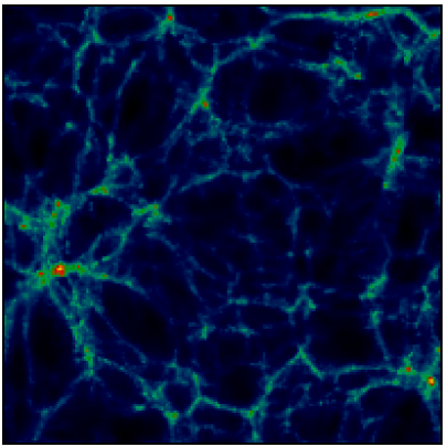
Figure 6.— Volume rendering of a thick slice of the density field in a $\Lambda$CDM simulation in a box of 200$h^{-1}$Mpc. Left: the full DTFE reconstructed density field. Right: the density field inside an isosurface at $\delta=1$.

5.3.3 Spine of the Voronoi Kinematic Model

The situation for the Voronoi Kinematic Model, marked by a more noisy particle distribution and a less idealized density field reconstruction, is less straightforward yet more representative for realistic circumstances.

Fig. 4 (righthand panel) shows, superimposed on the density field color map, the Voronoi particle distribution as well as the watershed transform. The latter is shown by means of the black lines. Particles identified as wall or filament particles are indicated by small diamonds. The watershed transform is able to identify most of the voids and their boundaries. The image shows that the SpineWeb procedure managed to closely follow the location of the edges and faces in the original Voronoi tessellation.

Some minor deviations are detected at small scales, the result of Poisson noise in combination with the discrete nature of the sampled density field. By construction, our filaments and walls are only one voxel thick (in this Voronoi model realization this is equal to $\sim 1h^{-1}\textrm{Mpc}$). As a result, we may miss the particles inside a given structure because of small-scale variations in the density field translating into variations in the watershed transform. This effect can be appreciated from the miss-classified (blue) particles in fig. 4, mostly clustered around the boundaries between filaments and filaments.

To determine the detection and contamination rate of the SpineWeb calculation, we compare the identity of the Voronoi wall and filament particles, which are a priori known from the model generation, with that of the classification on the basis of the reconstructed watershed segmentation. To this end, we assign the particles within a radius of $2\sigma\sim 2h^{-1}\textrm{Mpc}$ from a wall or a filament in the spine (watershed) segmentation to that particular structure: a particle is identified with a wall when it it lies within a $2\sigma$ distance from two different watershed cells. Although the detection rate results are less forthcoming than for the pure Voronoi element models, they remain convincing (see lower half of table 2. We find a detection rate of $76\%$ for wall particles, as opposed to a contamination rate of $\sim 32\%$. Filaments are better recognizable, which may be understood from the $87\%$ detection rate of filament particles, as opposed to a mere $13\%$ misclassification rate.

6. Single-scale $\Lambda$CDM Spine

To test the SpineWeb method in a more realistic and challenging situation we have applied it to a cosmological N-body simulation. It concerns a $\Lambda$CDM universe simulation inside a box of 200 $h^{-1}$ Mpc, restricted to the dark matter particles. Initial conditions were generated on a $512^{3}$ grid with $\Omega_{m}=0.3$, $\Omega_{\Lambda}=0.7$, $\sigma_{8}=0.9$ and $h=0.73$. For the primordial perturbations, we use the transfer function of Bardeen et al. (1986) with a shape parameter $\Gamma=0.21$ following the definition of Sugiyama (1995). After having set up the initial conditions, we follow the subsequent gravitational evolution to the present time using the public N-body code Gadget2 (Springel et al., 2005).

From the same initial conditions, we also generated additional lower-resolution versions of $256^{3}$, $128^{3}$ and $64^{3}$ particles were generated, following the “averaging” prescription described in (Klypin et al., 2001). For the single-scale analysis in this paper, which focuses on the largest filaments and walls in the particle distribution, it is sufficient to analyze the low-resolution $64^{3}$ dataset. The lower resolution corresponds to a cut-off scale of $\sim 3h^{-1}$Mpc in the initial conditions, sufficient for the analysis focusing on the large scale structure. The higher resolution datasets are used for visualization purposes.

6.1. Density field morphology

From the final particle distribution we compute the density field on a cubic grid of 512 voxels per dimension using the DTFE method (see sect. 4.1). Figure 6 (lefthand panel) depicts a volume rendering of the density field in a thick slice through the simulation box. It shows that DTFE manages to follow the intricacies of the weblike structures in great detail, over a range of scales: it reproduces the correct geometry of the various features.

An interesting example of structural complexities in the displayed region is the cluster at the lefthand side of the slice. A full 3D visualization of the system shows that the filaments entering the cluster define several semi-planar structures, all sharing the cluster as their common node. Lower isodensity contours reveal even more of the tenuous walls, even though at such low density levels we need to take into account that the image gets easily confused by spurious interloping features.

A frequently used approach for delineating structural features such as filaments and walls is to assign a specific density range to each morphology. Filaments or walls are singled out by selecting the regions that have a density within the corresponding density range. In the righthand panel of fig. 6 we show the density field inside an isodensity surface at $\delta=1$, for clarity superimposed on top of a white background. Because a density value $\delta=1$ is roughly comparable to typical values encountered in filaments and walls (see e.g. Aragón-Calvo et al., 2007), these contours roughly define the boundaries of the filaments and the clusters embedded, along with the tenuous walls suspended between the filaments.

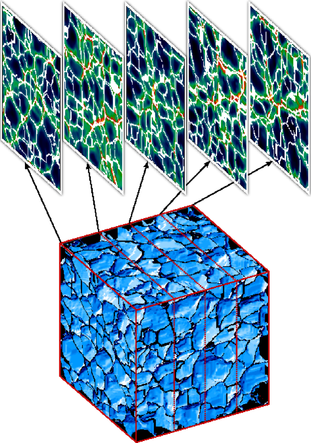
Figure 7.— Three-dimensional watershed transform of the density field. The cube shows the pixels that compose the watershed transform, from which the Spine is extracted. Several slices cut across the simulation box show the watershed (white lines) delineating the density field (blue-green background). The three dimensional nature of the watershed network is evident.

Although the isodensity surfaces provide good insight into the overall distribution of matter, one immediate observation is that the attempted pure density selection of filaments is not very successful. As was pointed out by Aragón-Calvo et al. (2007) filaments and walls are characterized by a rather broad range of densities (also see e.g. Hahn et al., 2007a). The broad cluster, filament, wall and field density ranges are also mutually overlapping over a sizeable density range (also see Aragón-Calvo et al., 2010c).

An immediate repercussion of the overlapping density ranges is that is almost impossible to decide purely on the basis of a density criterion whether a certain location belongs to a cluster node,filament or wall. This may be directly appreciated from the truncated density map in fig. 6. Although the image shows a substantial degree of filamentary structure, comparison with the full density field shows that it discards the pattern of lower density filaments. Also, it does not manage to disentangle the highly concentrated agglomeration of filaments near the massive cluster at the central lefthand side of the box. Moreover, throughout the whole volume it is rather difficult to see which locations would belong to a filament and which ones to a wall.

6.2. Cosmic Spine and Cellular Morphology

Following the computation of the density field, we compute its watershed transform. The resulting segmentation of the density field into its watershed basins is illustrated in figure 7.

The watershed basins are to be identified with the void regions in the cosmic matter distribution. To get a better idea of its spatial structure and the connections between the various structural components, we slice through the watershed field at regular intervals along the $x$-axis. This yields a sample of $yz$-slices through the simulation box. Figure 7 shows a sequence of five consecutive $yz$-slices, with the watershed segmentation shown as white lines superimposed on top of the density field (blue-green level) map. It is straightforward to appreciate the correspondence between the watershed segmentation lines and the underlying density field. While the segmented cube in figure 7 emphasizes the characteristic cellular nature of the Cosmic Web, the $yz$ slices reveal the close relationship between voids, walls and filaments.

The 2-D $yz$ slices show the strong correlation between the density field and the watershed transform. The watershed lines trace the high-density ridges and regions in the density field, occasionally bridging their lower-density connecting parts. On a more global scale, we also notice that the higher density regions contain a higher number of distinct and smaller cells than the more moderate or underdense areas. This translates into a more complex local network of filaments and walls. The opposite effect occurs in underdense regions. These are mainly characterized by large symmetrical voids, surrounded by relatively simple wall-filament environments.

Cosmic voids are immediately recognized as large empty cells in the watershed transform. The walls in the cosmic matter distribution are visible as the boundaries between two adjacent watershed cells, while the filaments are found at the intersection of these walls. The considerable variety of sizes and shapes of voids is most readily visible in the pattern of watershed lines in the $yz$-slices. Even though we know that on stereological grounds, lower-dimensional sections tend to exaggerate the size distribution of the full 3-D distribution, the comparison with the void basins in the 3-D box does confirm the impression of the diversity of the void population. It also underlines the significance of topological SpineWeb analysis: the void distribution is a direct reflection of the complexity of the dynamical processes which are forming and shaping the voids (Sheth & van de Weygaert, 2004; Platen et al., 2008).

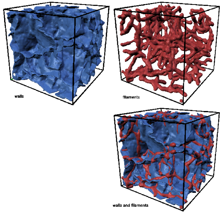
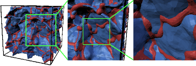
Figure 8.— Surfaces enclosing the voxels which are identified as belonging to walls (blue, top left) and filaments (red, top right) within a cubic region of $50h^{-1}$ Mpc. The bottom frame shows how in the same region both morphological components are connected and intertwined. The latter forms a nice illustration of the intimate relationship between filaments and walls. For visualization purposes the surfaces are smoothed with a Gaussian kernel of $\sigma=2$ voxels.

Figure 9.— Zoom-in onto the cosmic spine in a subregion of the $50h^{-1}$ Mpc, highlighting the intricate connections between wall surfaces (blue), filamentary edges and cluster nodes (red).

6.3. Cosmic Spine: Filaments and Walls

The final step in the SpineWeb method is to identify and label the voxels that correspond to the spine (filaments and clusters) and walls, following the SpineWeb criteria specified in equation 3.

An insightful impression of the intricacy of the full three-dimensional network of filaments and walls is presented in fig. 9. The top two frames show the wall-like (blue) and filamentary (red) regions separately. Clearly outstanding is the percolating nature of the filamentary network and the complex of connecting sheets.

The appearance of a uniform width, at places considerably in excess of the local width of the density field contours, is a result of our choice to show, for visualization purposes, a uniform smoothed outline. The plotted isosurface of both walls and filaments is obtained by filtering the mask defined by all wall voxels with a Gaussian kernel of $\sigma=2$ voxels. The Gaussian smoothing radius corresponds roughly to the average width of $\approx 2h^{-1}$Mpc of filaments and walls, as we found in a previous study (Aragón-Calvo et al., 2007). One may get an impression of the corresponding variation in density and width along the spinal structures by inspecting the two bottom frames of fig. 10, where we have superimposed density contour levels onto the embedding spinal contours (left: walls; right: filaments).

The top-left panels in figure  9 shows a network of complex sheets. Instead of a regular “planar” geometry, on small scales the walls have a curved appearance marked by an irregular surface. To a considerable extent this reflects their inhomogeneous internal mass distribution, itself a result of their hierarchical buildup. The irregular convoluted shapes are found on all scales, although the walls do have a slightly more regular semi-planar geometry on larger scales.

Also the filamentary structures reflect their inhomogeneous internal mass distribution, even though the applied smoothing has tended to diminish the contrast between e.g. massive clumps and tenuous moderate or lower density parts of the filaments. As a result, over most of its outline the filamentary edges look semi-linear. Nonetheless, occasionally we can recognize rather twisted configurations, and at numerous locations we can recognize the bulging presence of massive clusters. Taking the nodal junctions as the endpoints demarcating an individual filament, a first analysis shows that short filaments tend to be more straight than longer ones. This is entirely in line with the trend predicted by the Cosmic Web theory, and is in agreement with a corresponding analysis of N-body simulations (Bond et al., 1996; Colberg, Krughoff & Connolly, 2005; Nicholas10).

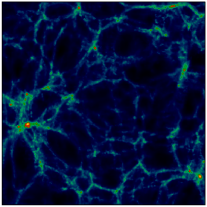
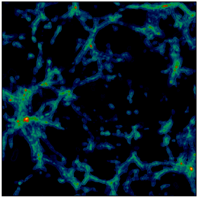
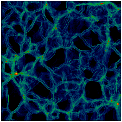
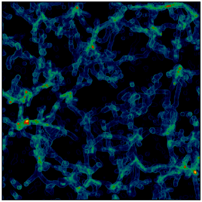
Figure 10.— Filaments and walls identified with the SpineWeb algorithm. Top left: Volume rendering of the density field inside a subbox of the simulation. Top right: density field contained inside an isosurface at $\delta=1$. Only the density inside the isocontour is plotted. Bottom left: density field and semi-transparent isosurfaces delineating walls. Bottom right: density field and semi-transparent isosurfaces delineating filaments. Both wall and filament mask have been smoothed for visualization purposes with a Gaussian filter of $\sigma=2$ pixels.

6.4. Morphological Connections

The close mutual relationship between the walls and filaments is immediately clear when inspecting the superposition of the wall-like and filamentary web in the bottom (right) frame of figure 9. With the filaments defining an interconnected web, the walls fill the spaces in between the filaments, together forming a “watertight” complex of membranes surrounding a system of voidlike cavities. The zoom-in onto one specific region centered around a particularly intricate branching of filaments emanating from a node, in fig. 9, highlights the complex connections that may occur in the Cosmic Web. At least four filaments appear to originate from a core region at the confluence of five walls. In the branches we can clearly recognize the bulging imprint of massive clusters. The zoom-in also nicely shows the small-scale heterogeneity of the walls’ surfaces.

6.5. Cosmic Spine versus Density Selection

To compare the morphological SpineWeb segmentation with the corresponding density field, in figure 10 we have depicted the matter distribution in a central slice through the simulation box. The two top panels are images of the density field (see discussion sect. 6.1), while the bottom panels present the density field within morphologically segregated regions. The two frames at the bottom show the density field inside semi-transparent surfaces enclosing the wall features (bottom left) and the filamentary features (bottom right).

6.5.1 Stereological Considerations

When assessing the bottom frame of fig. 10, we have to take into account that isolated features observed in these slices are the result of the finite thickness of the slice. Particularly noteworthy for the filaments in the righthand frame, they are artefacts of the finite width of the depicted slice. Because the orientation of filaments in the cosmic spine with respect to the slice is random, their intersection with the slice will differ. Dependent on the intersection angle, it may vary from their full length - in case they are nearly entirely embedded within the slice - to a mere point in case they run perpendicular to the slice. The resulting impression is one of a semi-irregular distribution of shorter and longer “stubs”, which indeed we find back in the bottom righthand frame.

The two-dimensional geometry of walls tends results in linear intersection with the depicted slice. This produces the fully percolating network of (intersection) edges seen in the bottom lefthand frame. Note that occasionally the orientation of a wall is so favorable that its intersection is not a one-dimensional edge but instead consists of a slab comprising a major fraction of the wall. In the most extreme circumstance, the wall is entirely embedded within the slice so that it remains visible in its entirety.

6.5.2 Morphological Structure of Density Features

While the first superficial impression might be that the isocontour map of the density field (see fig. 10 top-right panel) is richer in detail and structure than the filamentary and sheetlike morphologies in the bottom frames, a few important observations need to be made.

An important contrast between the isodensity contour maps and the filamentary and sheetlike networks defined by the SpineWeb procedure is that between the rather discontinuous nature of the (thresholded) density maps and the fully percolating spinal structure. This is most clearly visible when zooming in regions with large density contrasts, of which filaments close to the infall region are a good example. The massive cluster complex visible at the left of the box forms a nice illustration. The filamentary extensions connecting to the cluster are identified by the SpineWeb procedure (lefthand panel fig. 10), along with the sheetlike membranes of which they form the boundary (righthand panel fig. 10). It would be very challenging for traditional density-based filament detection techniques to trace filaments near cluster-filament interfaces. The density in the infall regions of clusters tends to increase dramatically, rendering a density-based criterion to determine the local morphology rather cumbersome(Aragón-Calvo et al., 2007).

7. Analysis Wall & Filament Sample

In this section we present a few quantitative measures of the voids, walls and filaments extracted by the SpineWeb technique. The results concern the single-scale analysis of our $64^{3}$ particle $\Lambda$CDM simulation described in the previous section (see sec. 6).

7.1. Density distribution

The density field of the $64^{3}$ simulation was computed on a regular 512³ grid, no smoothing was applied to the filament and wall masks. Figure 11 shows the density field distribution computed for the complete simulation box, voids, filaments and walls. The distribution of densities can be roughly described as log-normal with the main difference between morphological environments being the position of the peak of the distribution. Numerous studies have shown that a gravitationally evolving matter distribution, starting from Gaussian initial conditions, tends to attain a lognormal density distribution towards more advanced quasi-linear stages (Coles & Jones, 1991; Neyrinck et al., 2009; Platen, 2009). Our results indicate that this remains true for each of the individual morphologies.

Voids have the lowest densities followed by walls and filaments respectively. It is important to note that the network of filaments found by our method contains also the clusters which act as the nodes of the wall-filament network. This affects the right tail of the distribution and the computed moments. The median is a much better estimator than the mean in all cases given the effect of the clustering of matter into halos in our sampling schema.

Table 4 shows basic statistics of the density field characterized by the Spine. We present the statistic computed at two different grid resolutions ($256^{3}$ and $512^{3}$ voxels) as a simple convergence test. The numbers in table 4 show that the mean and median densities of the different morphologies are largely similar for the two different resolutions. This is quite different for the volume occupancy, in particular for the walls, filaments and clusters. This is a direct reflection of the resolution-dependent finite thickness assigned to filaments and walls, i.e. the voxel size. The volume fraction of voids is less sensitive to the grid resolution. We may understand this in terms of the SpineWeb invariants: void occupancy scales by volume, wall occupancy by surface area and filaments by length. The latter is therefore most sensitive to density field resolution, voids least.

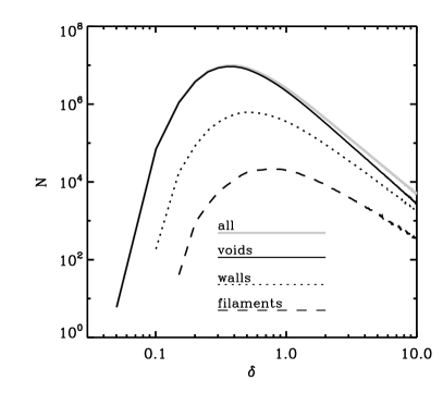
Figure 11.— Normalized density distribution for all voxels in the simulation box (thick gray line), void voxels (solid line), wall voxels (dotted line) and filament voxels (dashed line).

Table 3voids, filaments and walls: densities and volumes

Structure
	$(1+\delta)_{256}$		${\cal F}_{m,256}$
	mean	median
voids	0.81	0.56	0.825
walls	1.68	0.94	0.158
spine	3.46	1.58	0.015
	$(1+\delta)_{512}$		${\cal F}_{m,512}$
	mean	median
voids	0.86	0.58	0.889
walls	1.85	0.93	0.103
spine	4.47	1.57	0.006

Table 4Basic statistics of the density field in voids, walls and filaments, for density grids of $256^{3}$ (top) and $512^{3}$ (bottom) voxels. Quoted are the mean and median of the density field, $(1+\delta)$, in the individual morphologies, and the volume fraction ${\cal F}_{V,m}$ of each of them.

An important observation is also the considerable overlap between the pdf’s of the different morphologies. While distributions peak at clearly different places, there is a large overlap between all density distributions. This degeneracy in the density distributions between morphologies explains why a given isodensity contours does not manage to isolate one specific morphology, but will invariably include regions belonging to other morphologies too.

For our purpose, most significant are the differences between density distributions inside filaments and walls. Perhaps most remarkable is the sizeable overlap between densities in the void fields and those in filaments. The density distribution inside voids is almost identical to the overall density distribution. This is not surprising given the fact that even though voids are extremely underdense they occupy most of the space in the Cosmic Web. The difference between both distributions occurs at the high density tails where the clusters lie.

7.2. Minkowski-Bouligand dimension

We performed a preliminary scaling analysis of the identified filamentary and wall-like networks in the analyzed $\Lambda$CDM N-body simulation. To this end, we have determined for each of these networks the Minkowski-Bouligand dimension $D_{\textrm{\tiny{MB}}}$ – or box counting dimension – formally defined as:

$$D_{\textrm{\tiny{MB}}}\,=\,\lim_{\epsilon\rightarrow 0}\frac{\log N(\epsilon)}{\log(1/\epsilon)}.$$ (6)

In this expression, we count the number $N(\epsilon)$ of boxes of (infinitesimal) size $\epsilon$ required to fill or cover the set of points belonging to the filamentary or wall-like web. In practice, we divide the simulation box into subboxes of size $s$ and count the number $N(s)$ of subboxes that contain at least one voxel labeled as filament or wall. By repeating this evaluation for several box sizes, and determining the scaling index $N(s)\propto s^{-D}$, we obtain an estimate of the Minkowski-Bouligand dimension. One may visualize this by plotting the count $N(s)$ versus the size $s$ if the boxes, preferentially in a logarithmic diagram. If indeed characterized by a single fractal dimension, the resulting curve would be characterized by one slope. In practice, the structural patterns tend to be more complex, manifesting itself in scaling curves that cannot be characterized by a single uniform slope.

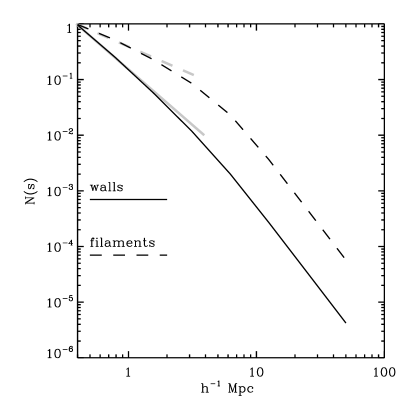
Figure 12.— Box-counting dimension of the filamentary spine (black dashed line) and walls (black solid line) of the Cosmic Web. For comparison we show the curves for ideal one and two-dimensional objects (gray dashed and gray solid lines respectively).

Figure 12 shows the Minkowski-Bouligand dimension computed for the wall and filament networks. We also show two (grey) lines with slope -1 and -2 as a reference indicating the cases of a pure one and two-dimensional objects. The slope of the curves for filaments and walls differ considerably at small scales. Filaments behave like one dimensional lines up to scales of $3-4$ $h^{-1}$Mpc after which point the absolute magnitude of the slope of the curve increases from -1 to -3 at scales of approximately 10 $h^{-1}$Mpc. In the case of the wall network we see a similar behavior with walls having a clear two-dimensional nature at scales smaller than $3-4$ $h^{-1}$Mpc. The transition point in the curve of figure 12 provides a good indication of the scale at which filaments and walls start joining each other forming an interconnected network. At this point their dimension is no longer 1 (filaments) or 2 (walls) but a higher value reflecting the complexity of the network of filaments and walls that form the Cosmic Web.

Figure 13.— Number of cells labeled as wall (left panel) or filament (right panel) inside boxes of $8$ $h^{-1}$Mpc of side as a function of the mean overdensity inside the $8$ $h^{-1}$Mpc box. The number of cells is normalized with the mean count of all the $8$ $h^{-1}$Mpc boxes.

7.3. LSS complexity and local density

Another measure of the local complexity of the network of filaments and walls is presented in figure 13 where we show the mean number of cells labeled as filament or wall inside boxes of $8$ $h^{-1}$Mpc size as a function of the mean density inside the boxes.

Low values indicate very simple local configurations while large values reflect complex environments. At first glance this may seem straightforward as increasing excursions sets of the density field have a similar behavior. However, the filaments and walls we identify are one-voxel thick so their voxel count correlates with their length and surface area respectively. For a given fixed volume larger counts indicate more intricate filament and wall systems.

We find a trend between the density and the complexity of the environment. Highly dense boxes tend to contain more structures than underdense boxes. The regions in the vicinity of massive clusters are a good example of complex neighborhoods defined in a locally overdense regions while the large voids define relatively simple wall and filament structures. The spread about the clearly visible mean trend is quite substantial. One of the main reasons is the restriction in the scale of the analysis, which leads to a confusion of intrinsic scales and counting of fainter structures together with more significant ones. A proper multiscale analysis, the subject of our following paper, will take this into account.

8. Conclusion and future work

The Spine of the Cosmic Web is the cosmic web’s framework, consisting of the network of filaments and walls and their connections at the clusters nodes. In this study we present a topological technique based on the discrete watershed transform of the cosmic density field for the identification and characterization of voids, walls and filaments. Our method is closely related to a variety of concepts from computational topology, and has a strong mathematical foundation in Morse theory of singularities.

The SpineWeb method is ideally suited for morphological and dynamical studies of the Large Scale Structure. Amongst others, it will allow a better insight into the formation and dynamics of the anisotropic filamentary and wall-like structures in the Large Scale Universe. Another immediate application is in addressing the question whether and which influences the large scale environment has on the halos and galaxies that are forming within their realm.

As a first test of its viability, we applied our method on a set of heuristic Voronoi clustering models. The SpineWeb procedure succeeds in reconstructing the original properties of the cellular galaxy distribution. In the implementation presented in this work, we effectively restrict ourselves to a single spatial scale determined by the voxel scale of the regular grid on which the density field is sampled. In a forthcoming paper we will discuss the effect of the multiscale nature of the matter distribution. The scale-space formulation of the SpineWeb method will enable us to identify fainter features in the density field and establish their connections with other objects into a truly hierarchical weblike pattern. In other words, it provides an effective way towards characterizing the hierarchy of structures in the Cosmic Web.

A crucial aspect of the watershed transform and of our method is the definition of local neighborhood. In the case of regular grids the immediate neighborhood of 26 pixels is arguably the best option. However, for unmeshed data such as galaxy surveys and N-body simulations, other neighborhood definitions offer a better choice. Among these, the Voronoi contiguous cell defined by the Delaunay tessellation of the point distribution represents a promising option. In the third paper of this series we will present the result of a Delaunay implementation of the Spine method.

9. Acknowledgments

We would like to thank Bernard Jones for inspiring discussions and insightful comments. This research was funded by the Gordon and Betty Moore foundation.

References

- Aragón-Calvo et al. (2007a) Aragón-Calvo M. A., van de Weygaert R., Jones B. J. T., van der Hulst J. M. 2007, ApJ, 655, L5
- Aragón-Calvo et al. (2007) Aragón-Calvo, M. A., 2007, Morphology and Dynamics of the Cosmic Web, PhD Thesis, University of Groningen, the Netherlands
- Aragón-Calvo et al. (2007b) Aragón-Calvo M. A., Jones B. J. T., van de Weygaert R., van der Hulst J. M. 2007, A&A, 474, 315
- Aragón-Calvo et al. (2010b) Aragón-Calvo M. A., Platen E, van de Weygaert R, Szalay A. 2009, in prep
- Aragón-Calvo et al. (2010c) Aragón-Calvo M. A., van de Weygaert R., Jones, B. J. T., van der Hulst J. M. 2009, MNRAS, to be subm.
- Bardeen et al. (1986) Bardeen J. M., Bond J. R., Kaiser N., Szalay A. S. 1986, ApJ, 304, 15
- Bertschinger (1987) Bertschinger E., 1987, ApJ, 323, 103
- Beucher (1982) Beucher, S., Watersheds of Functions and Picture Segmentation, 1982, ICASSP82, 1928-1931
- Beucher & Lantuejoul (1979) Beucher S., Lantuejoul C. 1979, In: Proceedings International Workshop on Image Processing, CCETT/IRISA, Rennes, France
- Bond et al. (1996) Bond J. R., Kofman L., Pogosyan D., 1996, Nature, 380, 603
- Bond et al. (2009) Bond N., Strauss M., Cen R., 2009, MNRAS, subm., arXiv:0903.3601
- Cayley (1859) Cayley A., 1859, On Contour and Slope Lines. The London, Edinburg and Dublin Philosophical Magazine and Journal of Science 18, 264-268
- Colberg, Krughoff & Connolly (2005) Colberg J.M., Krughoff K.S., Connolly A.J. 2005, MNRAS, 359, 272
- Colberg et al. (2008) Colberg J.M., Pearce F., Foster C., Platen E., Brunino R., Basilakos S., Fairall A., Feldman H., Gottlöber S., Hahn O., Hoyle F., Müller V., Nelson L., Neyrinck M., Plionis M., Porciani C., Shandarin S., Vogeley M., van de Weygaert R., 2008, MNRAS, 387, 933
- Coles & Jones (1991) Coles P., Jones B.J.T. 1991, MNRAS, 248, 1
- Colless et al. (2003) Colless M., et al 2003, arXiv:astro-ph/0306581
- Colombi et al. (2000) Colombi S., Pogosyan D., Souradeep T. 2000, Phys. Rev. Lett., 85, 5515
- Danovaro et al. (2003) Danovaro E.,De Floriani L., Magillo P., Mohammed M. M., Puppo E. 2003, In: GIS ’03, Proc. 11th ACM intern. symp. Adv. geographic information systems, ACM, 63
- Dolag et al. (2006) Dolag K., Meneghetti M., Moscardini L., Rasia E., Bonaldi A. 2006, MNRAS, 370, 656
- Du et al. (1999) Du Q., Faber V., Gunzburger M. 1999, SIAM Review, 41, 637-676
- Eberly (1994) Eberly D., Gardner R., Morse, B., Pizer S., Scharlach C. 1994, J. Math. Imaging and Vision 4, 353
- Edelsbrunner et al. (2001) Edelsbrunner H., Harer J., Zomorodian A. 2001, Proc. 17th ACM Symposium on Comp. Geometry, 70, ACM Press
- Edelsbrunner et al. (2003a) Edelsbrunner H., Harer J., Zomorodian A. 2003 , Discrete and Computational Geometry, 30, 87
- Edelsbrunner et al. (2003b) Edelsbrunner H., Harer J., Natarajan V. Pascucci V., 2003, SCG ’03: Proc. 19th ann. symp. Computational geometry, 361, 370
- Edelsbrunner (2010) Edelsbrunner H., Harer J., 2010, Computational Topology: An Introduction, AMS
- Forero-Romero et al. (2008) Forero-Romero J.E., Hoffman Y., Gottlöber S., Klypin A., Yepes G. 2008, MNRAS, 396, 1815
- Furst (2002) Furst J. D., Pizer S. M. 2002, Optimal parameter height rides. Journal of Visual Communication and Image Representation 13, 119-134
- Geller & Huchra (1991) Geller M.J., Huchra J.P. 1989, Science, 246, 897
- Giovanelli & Haynes (1985) Giovanelli R., Haynes M. P. 1985, AJ, 90, 2445
- Gregory et al. (1981) Gregory, S. A., Thompson, L. A., & Tifft, W. G. 1981, ApJ, 243, 411
- Gyulassy et al. (2005) Gyulassy, A., Natarajan, V., Pascucci, V., Bremer, P., Hamann, B. 2005, Proc. IEEE Conf. Visualization, p. 535
- Gyulassy (2008) Gyulassy A. 2008, Combinatorial Construction of Morse-Smale Complexes for Data Analysis and Visualization, Ph.D. Thesis, Univ. California Berkeley
- Hahn et al. (2007a) Hahn O., Porciani C., Carollo C. M., Dekel A. 2007, MNRAS, 375, 489
- Hahn et al. (2007b) Hahn O., Porciani C., Carollo C. M., Dekel A. 2007, MNRAS, 381, 41
- Hoffman & Ribak (1991) Hoffman Y., Ribak E., 1991, ApJ, 380, 5
- Huchra et al. (2005) Huchra J., et al. 2005, In: Nearby Large-Scale Structures and the Zone of Avoidance, ASP Conf. Ser. Vol. 239, eds. K.P. Fairall, P.A. Woudt (Astron. Soc. Pac., San Francisco), p. 135
- Icke (1973) Icke V. 1973, A&A, 27, 1
- Kirshner et al. (1981) Kirshner R. P., Oemler A. Jr., Schechter P. L., Shectman S. A. 1981, ApJ, 248, L57
- Klypin et al. (2001) Klypin A., Kravtsov A. V., Bullock J. S., Primack J. R. 2001, ApJ, 554, 903
- Magillo et al. (2007) Magillo P., Danovaro E., De Floriani L., Papaleo L., Vitali M. 2007, In: 2nd International Conference on Computer Graphics Theory and Applications (GRAPP’07)
- Maxwell (1870) Maxwell J. 1870, On hills and dales. The London Edinburg and Dublin Philosophical Magazine and Journal of Science 40, 412
- Martínez et al. (2005) Martínez V., Starck J.-L., Saar E., Donoho D.L., Reynolds S.C., de la Cruz P., Paredes S. 2005, ApJ, 634, 744
- Milnor (1965) Milnor J. 1965, Morse Theory, Princeton University Press
- Morse (1934) Morse M. 1934, The Calculus of Variations in the Large, American Mathematical Society Colloquium Publication, 18, New York
- Najman & Schmitt (1994) Najman L., Schmitt M. 1994, Signal Processing, 38:99-112
- Neyrinck (2008) Neyrinck M. 2008, MNRAS, 386, 2101
- Neyrinck et al. (2009) Neyrinck, M. C., Szapudi, I., & Szalay, A. S. 2009, ApJ, 698, L90
- Novikov et al. (2006) Novikov D., Colombi S., Doré O. 2006, MNRAS, 366, 1201
- Okabe (2000) Okabe A., Boots B., Sugihara K., Chiu S.N., 2000, 2nd ed., Wiley
- Park & Lee (2009) Park D., Lee J. 2009, MNRAS, in press, arXiv:0905.4277
- Peebles (1980) Peebles P. J. E. 1980, The Large-Scale Structure of the Universe, Princeton University Press, 1980.
- Platen et al. (2007) Platen E., van de Weygaert R., Jones B. J. T. 2007, MNRAS, 380, 551
- Platen et al. (2008) Platen E., van de Weygaert R., Jones B. J. T. 2008, MNRAS, 387, 128
- Platen (2009) Platen, E. 2009, A Void Perspective on the Cosmic Web, Ph.D. Thesis, University of Groningen, 2009
- Pogosyan et al. (1998) Pogosyan D.Yu., Bond J.R., Kofman L., Wadsley J. 1998, Cosmic Web: Origin and Observables. In: Wide Field Surveys in Cosmology, 14th IAP meeting), eds. S. Colombi, Y. Mellier, (Editions Frontieres, p. 61
- Pogosyan et al. (2009) Pogosyan D., Pichon C., Gay C., Prunet S., Cardoso J.F., Sousbie T., Colombi S. 2009, MNRAS, 396, 635
- Roerdink & Meijster (2000) Roerdink J. B. T. M., Meijster A. 2000, Mathematical Morphology, 41, 187–S28
- Schaap & van de Weygaert (2000) Schaap W. E., van de Weygaert R. 2000, A&A, 363, L29
- Schaap (2007) Schaap, W. E. 2007, The Delaunay Tessellation Field Estimator, Ph.D. Thesis, University of Groningen
- Shannon E. C. (1948) Shannon, E. C. 1948, Bell System Technical Journal, Vol. 27, pp. 379–423, 623–656
- Sheth & van de Weygaert (2004) Sheth R., van de Weygaert R., 2004, MNRAS, 350, 517-538
- Sousbie et al. (2008a) Sousbie T., Pichon C., Colombi S., Novikov D., Pogosyan D. 2008, MNRAS, 383, 1655
- Sousbie et al. (2008b) Sousbie T., Pichon C., Courtois H., Colombi S., Novikov D. 2008, ApJ, 672, 1
- Sousbie et al. (2009) Sousbie T., Colombi S., Pichon C. 2009, MNRAS, 393, 457
- Springel et al. (2005) Springel V., White S.D.M., Jenkins A., Frenk C.S., Yoshida N., Gao L., Navarro J., Thacker R., Croton D., Helly J., Peacock J.A., Cole S., Thomas P., Couchman H., Evrard A., Colberg J.M., Pearce F. 2005, Nature, 435, 629
- Stanonik et al. (2010) Stanonik K., Platen E., Aragón-Calvo M.A., van Gorkom J., van de Weygaert R., van der Hulst J.M., Kovac̆ K., Yip C.-W., Peebles P.J.E. 2010, ApJ, subm.
- Stoica et al. (2005) Stoica, R. S., Martínez, V. J., Mateu, J., & Saar, E. 2005, A&A, 434, 423
- Sugiyama (1995) Sugiyama, N. 1995, ApJS, 100, 281
- van de Weygaert & Icke (1989) van de Weygaert, R., Icke, V. 1989, A&A, 213, 1
- van de Weygaert & Bertschinger (1996) van de Weygaert, R., Bertschinger, E. 1996, MNRAS, 281, 84
- van de Weygaert (2002) van de Weygaert R. 2002, Froth Across the Universe. Dynamics and Stochastic Geometry of the Cosmic Foam. In: Modern Theoretical and Observational Cosmology, proc. 2nd Hellenic Cosmology Meeting, ed. by M. Plionis, S. Cotsakis, ASSL 276 (Kluwer)
- van de Weygaert & Bond (2008a) van de Weygaert R., Bond J.R. 2008, Clusters and the Theory of the Cosmic Web. In: A Pan-Chromatic View of Clusters of Galaxies and the Large-Scale Structure, eds. M. Plionis, O. Lopez-Cruz, D. Hughes, Lect. Notes Phys., 740, 335 (Springer)
- van de Weygaert & Bond (2008b) van de Weygaert R., Bond J.R. 2008, Observations and Morphology of the Cosmic Web. In: A Pan-Chromatic View of Clusters of Galaxies and the Large-Scale Structure, eds. M. Plionis, O. Lopez-Cruz, D. Hughes, Lect. Notes Phys., 740, 409 (Springer)
- van de Weygaert & Schaap (2009) van de Weygaert R., Schaap W.E 2009, The Cosmic Web: Geometric Analysis. In: Data Analysis in Cosmology, eds. V. Martínez et al., Lecture Notes Phys., 665, 291-413 (Springer-Verlag)
- van de Weygaert & Schaap (2009) van de Weygaert R., Schaap W.E 2009, The Cosmic Web: Geometric Analysis. In: Data Analysis in Cosmology, eds. V. Martínez et al., Lecture Notes Phys., 665, 291-413 (Springer-Verlag)
- van de Weygaert (2010) van de Weygaert R. 2010, Voronoi Clustering Models of the Cosmic Web. In: Tessellations in the Sciences; Virtues, Techniques and Applications of Geometric Tilings, eds. R. van de Weygaert, G. Vegter, J. Ritzerveld, V. Icke (Springer-Verlag)
- Voronoi (1908) Voronoi G., 1908, J. Reine Angew. Math., 134, 198
- Zeldovich (1970) Zel’dovich Y. B., 1970, A&A, 5, 84
- Zitrin & Brosch (2009) Zitrin A., Brosch N. 2009, MNRAS, 390, 408