ULB-TH/08-30

Baryon Dissociation in a Strongly Coupled Plasma

Chethan KRISHNAN

International Solvay Institutes,
Physique Théorique et Mathématique,
ULB C.P. 231, Université Libre de Bruxelles,
B-1050, Bruxelles, Belgium

Abstract

Using the dual string theory, we study a circular baryonic configuration in a wind of strongly coupled ${\cal N}=4$ Yang-Mills plasma blowing in the plane of the baryon, before and after a quark has dissociated from it. A simple enough model that captures many interesting features is when there are four quarks in the baryon. As a step towards phenomenology, we compare representative dissociated configurations, and make some comments about their energetics and other properties. Related results that we find include the observation that the screening length formula $L_{s}T\sim(1-v^{2})^{1/4}$ obtained previously for other color singlet configurations, is robust for circular baryons as well.

KEYWORDS: AdS/CFT correspondence, QCD, Thermal Field Theory

1 Introduction and Conclusion

There is a possibility that screening of heavy quark baryons in a wind of strongly coupled plasma might be experimentally accessible at RHIC or LHC. Unfortunately, this is a deeply non-perturbative scenario in standard QCD, and therefore essentially out of theoretical control. Interestingly enough, semi-quantitative features of baryon screening can be computed using a dual string theory through the AdS/CFT correspondence [1]. This has resulted in some non-trivial progress in the understanding of screening phenomena in strongly coupled plasmas [2, 3, 4, 5].

In a wind of plasma, the screening is direction-dependent, and it stands to reason that when the baryon dissociates, there will be preferred directions in which this can happen first. The purpose of this paper is to explore this possibility by computing some basic energetics. This should be taken as a small step towards phenomenology.

As a warmup, we first compute the (regulated) energy of a circular baryonic configuration with $N_{c}=4$ quarks (attached in the bulk to a D5-brane baryon vertex wrapping the $S^{5}$), moving in a hot, strongly coupled, ${\cal N}=4$ plasma. For a generic baryon configuration, this can be done using worldsheet string theory in $AdS_{5}\times S^{5}$, with a black hole in the interior. Our results about these baryons also serve as a test of robustness of the known results in the literature. After this, we calculate the energy of the configuration after one of the quarks has dissociated from the baryon and is well-separated. Both the quark, and what remains of the baryon, will have trailing strings reaching down to the black hole horizon. There are many such dissociated configurations, and we will try to get some intuition for them by considering some special cases. Among these will be two extreme scenarios: one when the remaining three quarks are spaced equidistantly in a line along the wind (case I), and the other when the quarks (again spaced equidistantly along a line) are perpendicular to the wind (case II). The “dynamics” of the system is sufficiently stringent that for the configurations we consider, we will be able to explicitly do the computations without getting tangled up in too many details.

We stress that our aim is not to identify preferred dissociation channels and do any detailed phenomenology. This would be a tall order. Our aim is merely to see whether something can be said about energetics of transverse configurations vs. longitudinal ones. The two specific cases we consider are chosen with this specific purpose in mind, and they are not supposed to necessarily be the preferred dissociation products. In fact, one might think that the “natural” dissociated configurations are instead the ones we consider in Appendix C. But this is so only if one assumes that the remaining quarks stay on the circle. The problem here is that “natural” is not very well-defined, because the dynamics is not under control and all we are dealing with are static configurations.

In any event, we find that the energy of the configuration with quarks parallel to the wind (case I) is at a higher energy than case II, and therefore it is tempting to speculate that for baryons in a wind of plasma, the quarks along the wind will dissociate first. We emphasize that the computations we do should not be taken as a proof of this claim, even though we believe they are suggestive. In particular, it is not clear what configurations constitute extreme cases. It is a complicated dynamical question whether a configuration would prefer to change the dimension (i.e., change the length $L$) and/or change the orientation in order to lower its energy. But it can still be instructive to have a comparison of identical configurations with different orientations: naively, one might think that for a given dimension, a transverse configuration is at a higher energy because it has more cross-section to the wind. Our results show that this is not the case. Also, there are speculations and comments in the literature about the relative energetics of transverse-vs.-longitudinal cases. Such statements make most sense only if one assumes that we are comparing two configurations of identical dimensions, and this is what we do.

In general, the features of a dissociated baryon are likely to depend strongly on the specific configurations under consideration, and making generic claims is difficult. To emphasize this, we compute the energetics of some other dissociated configurations in an appendix.

A more detailed computation where the number of quarks and the possible dissociation channels are increased will certainly be useful in shedding more light on similar questions. It would be interesting to do a full scan in the the space of allowed dissociated configurations, but this is numerically a more demanding problem than what we have undertaken in this paper. It should also be pointed out that conclusive evidence might require an understanding of the dynamics of dissociation patterns which our static calculation is blind to: in principle, it is always possible for instance that the configuration can rotate or dilate during or after a dissociation process.

In the course of the computations in this paper we learn a few things about dragging and non-dragging objects and these will be elaborated upon as and when they arise. Among these is the observation that the screening length formula found previously in the literature for other color singlet configurations, $L_{s}T\sim(1-v^{2})^{1/4}$, is valid for circular baryons as well. This is interesting because the details of the configurations and the computations are quite different in our case. Another thing we find is that the plots of $E$ vs. $L$ for non-dragging objects exhibit a cusp while those of dragging configurations exhibit a loop, and we speculate that the area of the loop is a measure of the drag of the configuration. This could potentially be a measure of the energy loss.

In this paper, we only consider the simplest possible scenario: a baryon that is simulated by a circular configuration of four (external) quarks in the maximally symmetric gauge theory, with the added simplification that the plasma is flowing in the plane of the baryon. But it is possible to consider generalizations of the results here to more generic baryon configurations, less special gauge theories and perhaps more generic wind directions. It would be interesting to see how generic the results are. Some papers that are relevant (from various angles) to hot strongly coupled QCD are [11, 12, 13, 14, 15, 16, 17, 18, 19, 20, 21, 22, 23].

2 Baryon Screening and the AdS Black Hole

Baryons are made out of fundamental quarks in QCD, but the field content of the ${\cal N}=4$ supersymmetric Yang-Mills theory consists of gluons, gluinos and scalars (all in the adjoint); but not quarks. So in order to model QCD phenomena, we introduce baryons that are constructed out of external quarks. If the ${\cal N}=4$ SYM theory has $N_{c}$ colors, the baryons will be constructed from $N_{c}$ such external quarks.

The dynamics of baryons in the gauge theory is captured in the dual $AdS_{5}\times S^{5}$ string theory through the introduction of the so-called baryon vertex [6]. The claim is that baryons in the gauge theory are dual to configurations that involve a D5-brane wrapping an $S^{5}$ in the bulk, with all the heavy external quarks in the boundary baryon being linked to it through fundamental strings (all of which are of the same orientation).

The way in which we make predictions for a baryon moving in the plasma is by boosting to the rest frame of the baryon and letting the plasma move instead. In the dual picture, we look for static baryon configurations in the boosted bulk metric. In the course of this paper, we will be exclusively working with the case of ${\cal N}=4\ {\rm SYM}$, with the plasma at a temperature $T$. Finite temperature implies that the asymptotics of the bulk is still $AdS_{5}\times S^{5}$ but in the interior we have to change the metric to include a black hole whose Hawking temperature is $T$ [7]. Before the boost, this bulk AdS black hole metric takes the form

$$ds^{2}=-f(r)dt^{2}+\frac{r^{2}}{R^{2}}d\vec{x}^{2}+\frac{dr^{2}}{f(r)}+R^{2}d\Omega_{5}^{2},$$ (2.1)

with

$$f(r)=\frac{r^{2}}{R^{2}}\left(1-\frac{r_{0}^{4}}{r^{4}}\right).$$ (2.2)

The asymptotic boundary where the field theory lives is supposed to be at $r\rightarrow\infty$, and is spanned by $\vec{x}=\{x_{1},x_{2},x_{3}\}$ and the bulk-time $t$. In the above, $r_{0}$ is the black hole horizon and the temperature $T$ is fixed by the Hawking relation $T=\frac{r_{0}}{\pi R^{2}}$. The standard CFT to AdS correspondence is usually expressed by taking the defining parameters of the gauge theory to be $\lambda\ (\equiv g^{2}_{YM}N_{c})$ and $N_{c}$. Then, the bulk data is related to the boundary data through Maldacena’s famous relations

$$\frac{\lambda}{N_{c}}=4\pi g_{s},\ \sqrt{\lambda}=\frac{R^{2}}{\alpha^{\prime}},$$ (2.3)

with $g_{s}$ the string coupling and $\frac{1}{2\pi\alpha^{\prime}}$ the worldsheet tension. The Maldacena conjecture can be taken as the claim that string propagation with these parameters in the AdS background (with a background five-form flux controlled by $R$) is just another description of the gauge theory.

We will take the plasma wind to be in the $x_{3}$-direction after the boost, and the velocity and rapidity are related by $v=-\tanh\eta$. The boosted metric takes the form

$$ds^{2}=-Adt^{2}+2B\,dt\,dx_{3}+C\,dx^{2}_{3}+\frac{r^{2}}{R^{2}}\left(dx^{2}_{1}+dx^{2}_{2}\right)+\frac{1}{f(r)}dr^{2}+R^{2}d\Omega^{2}_{5}\,.$$ (2.4)

The various quantities are fixed by,

$$A=\frac{r^{2}}{R^{2}}\left(1-\frac{r^{4}_{1}}{r^{4}}\right),\qquad B=\frac{r^{2}_{1}r^{2}_{2}}{r^{2}R^{2}},\qquad C=\frac{r^{2}}{R^{2}}\left(1+\frac{r^{4}_{2}}{r^{4}}\right),$$ (2.5)

and

$$r^{4}_{1}=r^{4}_{0}\cosh^{2}\eta,\quad\textrm{and}\quad r^{4}_{2}=r^{4}_{0}\sinh^{2}\eta.$$ (2.6)

Our description of the baryon-like configurations will involve the baryon vertex (the D5-brane), and various strings emanating from the baryon vertex and ending on the asymptotic boundary or the black hole horizon. The actions of the string worldsheets and the D5-brane can be used to determine static solutions to the equations of motion. We will work below in the restricted context of the AdS black hole described above, a more general formulation can be found in [5].

In this section, we will illustrate the method by explicitly working out the relevant physics of an $N_{c}=4$ baryon moving in the plasma. This example is also our prime workhorse. The conflict between setting $N_{c}=4$ and the desire to have a large $N_{c}$ planar approximation where finite string coupling effects are suppressed does not seem to be too much, because as we will see, the various results that were found in [5] can be reproduced in our case as well. In particular, in [5], large $N_{c}$ squashed baryons were considered, and the curves that we find later in this section are in excellent agreement with their work. So we believe that we are not throwing the baby out with the bath water by studying this simple system. Adding more quarks is in principle straightforward, except that the computational effort is, of course, more.

The configuration we wish to study is shown in Figure 1. The circular configuration of quarks lies in the $x_{1}$-$x_{3}$ plane and the plasma wind is in the $x_{3}$ direction. In the figure we have suppressed all coordinates except $r,x_{1}$ and $x_{3}$.

Figure 1: The $N_{c}=4$ baryon configuration in the AdS black hole background. The baryon vertex is at $r=r_{e}$.

The action for the system is given by

$$S=S_{1}+S_{2}+S_{3}+S_{4}+S_{D5},$$ (2.7)

where subscripts denote the various strings and the D5-brane. The actions for the various strings are computed à la Nambu-Goto in the black hole background:

$$S_{NG}=\frac{1}{2\pi\alpha^{\prime}}\int d\sigma d\tau\sqrt{-g_{\alpha\beta}},\ {\rm with}\ g_{\alpha\beta}=G_{\mu\nu}\partial_{\alpha}x^{\mu}\partial_{\beta}x^{\nu},$$ (2.8)

where $G$ is the black hole metric and $g$ is the induced worldsheet metric. If we assume that the configuration experiences no drag, we can look for axially symmetric circular configurations like the one shown in Figure 1. For the two strings in the $x_{1}$ direction, then, we can take the embedding to be

$$\tau=t,\ \ \ \sigma=r,\ \ \ x^{(a)}_{1}=x^{(a)}_{1}(\sigma)$$ (2.9)

where $a$ is either 2 or 4 and denotes the appropriate string (see Figure 1). No $\tau$ dependence arises because we are interested in static configurations. The action for the strings takes the form

$$S_{a}=\frac{{\cal T}}{2\pi\alpha^{\prime}}\int_{r_{e}}^{\infty}dr\sqrt{A\left(\frac{1}{f}+\frac{r^{2}}{R^{2}}\left({x^{(a)}_{1}}^{\prime}\right)^{2}\right)},\ \ \ a=2,4,$$ (2.10)

where $\cal T$ can be thought of as the total time which gets divided out in any relevant quantity. Primes denote derivatives with $r$. In the above expression, $r_{e}$ is the position of the baryon vertex and it can lie anywhere between $r=r_{0}$ and $r=\infty$, i.e., between the boundary and the horizon. The boundary conditions for the string coordinates are fixed by the condition that the baryon vertex has coordinates $(r=r_{e},x_{1}=0,x_{3}=0)$. At the boundary, from a glance at the figure, we see that $x^{(2)}_{1}(\infty)=-L$ and $x^{(4)}_{1}(\infty)=L$, where $L$ is the radius of the circle. For the strings in the $x_{3}$-directions, similarly, we get

$$S_{b}=\frac{{\cal T}}{2\pi\alpha^{\prime}}\int_{r_{e}}^{\infty}dr\sqrt{\left(\frac{A}{f}+\frac{r^{2}}{R^{2}}f\left({x^{(b)}_{3}}^{\prime}\right)^{2}\right)},\ \ \ b=1,3.$$ (2.11)

The boundary conditions at infinity are given by $x^{(1)}_{3}(\infty)=L,x^{(3)}_{3}(\infty)=-L$. The action for the D5-brane vertex can be taken as [5]

$$S_{D5}=\frac{N_{c}R{\cal T}}{8\pi\alpha^{\prime}}\sqrt{A(r_{e})}.$$ (2.12)

2.1 Energetics and Screening Lengths

The equations of motion for the configuration are obtained by varying the total action with respect to the $x(r)$’s and also with respect to the location of the D5-brane. The details have been worked out in [5] and the result adapted to our case takes the following form. (We suppress the string number superscripts $a(=2,4),b(=1,3)$ in some of the equations below.)
Strings 1, 3:

$$\left(x_{3}^{\prime}\right)^{2}=\frac{R^{4}}{f^{2}r^{2}}\frac{K_{3}^{2}A}{\left(r^{2}f-R^{2}K_{3}^{2}\right)},\ \ x_{1}^{\prime}=0.$$ (2.13)

The $K_{3}$ are integration constants. The $K_{3}$ have to satisfy the condition,

$$K_{3}^{(1)}+K_{3}^{(3)}=0,$$ (2.14)

as a force balance condition on the D5-brane. So we effectively need to solve only for one of the strings.
Strings 2, 4:

$$\left(x_{1}^{\prime}\right)^{2}=\frac{R^{4}}{r^{2}}\frac{K_{1}^{2}}{f\left(r^{2}A-R^{2}K_{1}^{2}\right)},\ \ x_{3}^{\prime}=0.$$ (2.15)

Again there is the relation

$$K_{1}^{(2)}+K_{1}^{(4)}=0$$ (2.16)

that has to be satisfied.
D5-brane:

$$\frac{2R\sqrt{A}}{\sqrt{f\left(R^{2}+fr^{2}(x_{1}^{\prime})^{2}\right)}}\biggr{|}_{r=r_{e}}+\frac{2RA}{\sqrt{f\left(AR^{2}+f^{2}r^{2}(x_{3}^{\prime})^{2}\right)}}\biggr{|}_{r=r_{e}}=\frac{r_{e}^{4}+r_{1}^{4}}{r_{e}^{2}\sqrt{r_{e}^{4}-r_{1}^{4}}}$$ (2.17)

It should be noted that this equation is evaluated at $r=r_{e}$. Since the string equations written down above depend only on the square of the $K$’s, and these squares are identical for both strings in each pair, we don’t specify the superscript in the $x_{1}^{\prime}$ and the $x_{3}^{\prime}$ in the D5-brane equation.

By introducing new variables, we can write these in the equivalent form

$$L=\frac{\rho\ \beta}{\pi T}\int_{1}^{\infty}dy\frac{1}{(y^{4}-\rho^{4})}\sqrt{\frac{y^{4}-\rho^{4}\cosh^{2}\eta}{y^{4}-\rho^{4}-\beta^{2}}},$$ (2.18)

$$L=\frac{\rho\ \alpha}{\pi T}\int_{1}^{\infty}\frac{dy}{\sqrt{(y^{4}-\rho^{4})(y^{4}-\rho^{4}\cosh^{2}\eta-\alpha^{2})}},$$ (2.19)

$$\frac{\sqrt{1-\rho^{4}\cosh^{2}\eta}\sqrt{1-\rho^{4}-\beta^{2}}}{(1-\rho^{4})}+\frac{\sqrt{1-\alpha^{2}-\rho^{4}\cosh^{2}\eta}}{\sqrt{1-\rho^{4}}}=\frac{1+\rho^{4}\cosh^{2}\eta}{2\sqrt{1-\rho^{4}\cosh^{2}\eta}}.$$ (2.20)

We have integrated the string equations of motion while imposing the boundary condition that the radius of the circle is $L$ at the asymptotic boundary. In the process we have also introduced the notation

$$\alpha^{2}=\frac{K_{1}^{2}R^{4}}{r_{e}^{4}},\ \ \beta^{2}=\frac{K_{3}^{2}R^{4}}{r_{e}^{4}},\ \ y=\frac{r}{r_{e}},\ \ \rho=\frac{r_{0}}{r_{e}}.$$ (2.21)

To extract information about the baryon we need to solve these three equations simultaneously. This can be done numerically.

• Pick a value for $\eta$ first.

• Now, for each $\rho$ (it is easy to see that $\rho$ must lie in the range $(0,1)$ from the geometry) we can solve for $\beta$ in terms of $\alpha$ as we vary $\alpha$ (which again has to be between $0$ and $1$.).

• The correct value of $\alpha$ for each $\rho$, is the one where the $\alpha$-integral matches the $\beta$-integral.

• The value of the integral(s) at which this match happens is the value of $L$.

• Repeat the above procedure for another value of $\eta$.

Plot of $L$ as a function of $\rho$ are presented here, for a few values of $\eta$. The plot for $L$ has a peak, and this is what one identifies as the screening length, $L_{s}$. The results here match perfectly with those in [5].

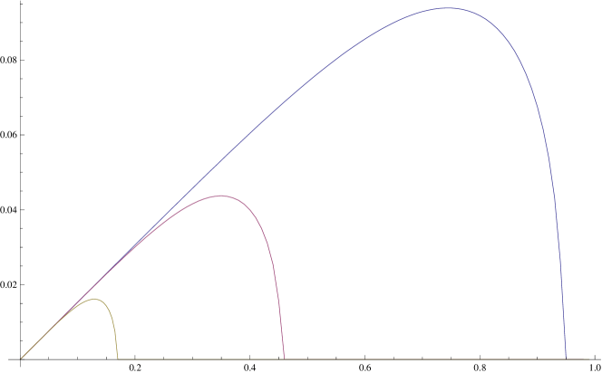
Figure 2: $LT$ vs. $\rho$ for $\eta=0\ ({\rm top\ curve}),2,4\ ({\rm bottom\ curve})$. The maximum is associated to the screening length $L_{s}$ at the corresponding $\eta$.

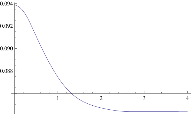
Figure 3: $L_{s}T\sqrt{\cosh\eta}$ vs. $\eta$.

The dependence of $L_{s}$ on the rapidity $\eta$ can also been plotted, and the result again agrees with expectations from other baryonic and mesonic configurations considered previously in the literature. In particular, it is evident from this plot that $L_{s}T\sim(1-v^{2})^{1/4}$ for large boosts, and this is a check of the robustness of this result.

In the bulk of this paper, however, energetics are more interesting to us than screening lengths, so we turn to the computation of energy. The total energy is the sum of the various pieces, with the caveat that the energy of each string in the baryon needs to be regulated by subtracting the energy of a free string stretching all the way from the boundary to the horizon. Before the regularization, the total energy is given by the (formal) expression

$$E=\frac{1}{\pi\alpha^{\prime}}\int_{r_{e}}^{\infty}dr\sqrt{\frac{A}{f}+\frac{r^{2}f}{R^{2}}\left({x_{3}}^{\prime}\right)^{2}}+\frac{1}{\pi\alpha^{\prime}}\int_{r_{e}}^{\infty}dr\sqrt{\frac{A}{f}+\frac{r^{2}A}{R^{2}}\left({x_{1}}^{\prime}\right)^{2}}+\frac{R}{2\pi\alpha^{\prime}}\sqrt{A(r_{e})}$$

Factors of two have been put in to take account of the two strings in each pair. The last piece is the energy of the D5-brane. The energy of the regulator quark has been calculated in the literature, we will use the expression (A.10) from [4]. The idea is to cut off the energy integral written above at $\Lambda$ instead of $\infty$, subtract the quark energy integrated from the horizon to the cutoff, and then take the limit $\Lambda$ to infinity after the subtraction. The result is,

$$E=T\sqrt{\lambda}\Biggl{[}\frac{1}{\rho}\int_{1}^{\infty}dy\left(\sqrt{\frac{y^{4}-\rho^{4}\cosh^{2}\eta}{y^{4}-\rho^{4}-\beta^{2}}}-1\right)+1-\frac{1}{\rho}+\hskip 50.58878pt$$ (2.22)

$$+\frac{1}{\rho}\int_{1}^{\infty}dy\left(\frac{y^{4}-\rho^{4}\cosh^{2}\eta}{\sqrt{(y^{4}-\rho^{4})(y^{4}-\rho^{4}\cosh^{2}\eta-\alpha^{2})}}-1\right)+1-\frac{1}{\rho}+\frac{\sqrt{1-\rho^{4}\cosh^{2}\eta}}{2\rho}\Biggr{]}.$$

where we have used the variables 2.21 as well as Maldacena’s relations and the geometrical definition of the Hawking temperature.

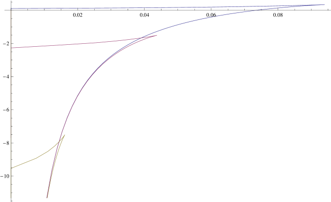
Figure 4: $\frac{E}{T\sqrt{\lambda}}$ vs. $L$, for $\eta=0\ ({\rm top\ curve}),2,4\ ({\rm bottom\ curve})$.

With the values of $L$, $\alpha$, $\beta$ that we computed earlier, it is possible to make a numerical plot between $L$ and $E$ for various values of $\eta$ and we present the results in the figure. This ties in as it should, with the similar plot in [5].

The computations of this section serve two purposes. Firstly and primarily for us, they give a context for the rest of the work on this paper. But in the process, they also provide a confirmation of the robustness of previous results on baryons. In [5], qualitatively identical results were observed, where instead of keeping the baryons on a circle, the angle at which the strings hit the D5-brane was fixed. This amounts to considering quark configurations that are squashed in the plasma wind. This makes the computations technically different, but still we see from a glance at the plots that the essential features are identical and therefore that the results are indeed very robust. In particular, the screening length formula $L_{s}T\sqrt{\cosh\eta}\sim{\rm const.}$ holds in our case as well for large $\eta$, even though the value of the constant seems slightly different.

3 Dissociated Baryons

Clearly there are many possible ways in which the baryon presented in the previous section can dissociate. One possibility is to look at configurations where one quark has dissociated, while keeping as many of the remaining quarks as possible still on the circle. After the force balance conditions are imposed on the D5-brane, there are only a few interesting configurations which one can consider in this manner (we will look at them in Appendix C). But since the process of ripping a quark is fundamentally dynamical, it is not clear to us that such configurations where the quarks are forced to be in a circle are the only ones preferred. Since it is difficult to come up with an unambiguous definition of what is “closest” and what is “farthest” to the original baryonic configuration, we will attempt something more modest here. We will instead consider two baryonic configurations with identical linear dimensions but different orientations. We hope to make some comments about their relative energetics from this, but notice that we are steering clear of the question of what are the preferred dissociation products.

The two configurations we consider are as follows. One is when the undissociated quarks are in a rigid identically spaced line parallel to the wind (i.e., along $x_{3}$) (case I), and the other is when they are in the direction perpendicular to the wind (i,e., along $x_{1}$) (case II). We will also have a dissociated string in each case, which we will take to be well-separated from the rest of the baryon. Our aim is to look at two configurations that are identical, except for their orientation in the wind. Even though we will need to work much harder to get a fuller understanding of phenomenology, to get a hint about the orientation-dependence of the energy, this computation should be enough.

We address both the cases separately. But before doing so, we notice a useful fact: the dissociated string that trails all the way to the horizon from the D5-brane is forced to lie along $x_{3}$. This is demonstrated in Appendix B.

3.1 Case I: Longitudinal Quarks

We first consider the case where the undissociated quarks are along the direction of the wind. After the dissociation, the string corresponding to the dissociated quark is trailing, with one of its endpoints at the D5-brane vertex and the other at the horizon. The configuration we are considering is demonstrated in figure 5, and consists of three quarks in a straight-line. In case II, we will consider three quarks, again in a straight line, but perpendicular to the wind. The hope is that these two complimentary configurations will give us some idea about the energetics. Notice that because of the constraints arising from force balance at the D5-brane and because the trailing string is forced to lie along $x_{3}$, many of the configurations are ruled out. An advantage of comparing the two cases we consider here is that they give a natural way to contrast between the cases: we can compare quark configurations of equal linear dimensions on either side. This is useful in getting some insight about how the energy of a given configuration (with fixed linear dimensions) changes with the orientation.

Figure 5: Case I: Remnant with quarks along the plasma wind.

We can compute the energy of this configuration using methods similar to those of last section. In what follows, $\beta_{i},\alpha_{i}$ are defined as in the last section (the indices in the present case denote the respective quark). In case I, the $\alpha_{i}$ are identically zero. The origin of the coordinate system is taken to be at the D5 brane ($x_{1}(D5)=x_{3}(D5)=0$). The numbering of the quarks are indicated in the figure. The trailing string solution forces the relation

$$\beta_{4}=\rho^{2}\sinh\eta.$$ (3.1)

Using the results of Appendix A, we can write down the vertical force balance condition at the D5-brane as

$$\frac{\sqrt{1-\rho^{4}\cosh^{2}\eta}}{1-\rho^{4}}\left(\sum_{i=1}^{3}\sqrt{1-\rho^{4}-\beta_{i}^{2}}-\sqrt{1-\rho^{4}-\beta_{4}^{2}}\right)=\frac{1+\rho^{4}\cosh^{2}\eta}{\sqrt{1-\rho^{4}\cosh^{2}\eta}},$$ (3.2)

and the horizontal balance as,

$$\beta_{1}+\beta_{2}+\beta_{3}=\beta_{4}(=\rho^{2}\sinh\eta).$$ (3.3)

In case I, we will look at configurations with the three undissociated quarks placed equidistantly on a line, along the wind. Thus we have the two equations below for the distance between quarks.

$$L_{12}\equiv L=\frac{\rho}{\pi T}\int_{1}^{\infty}dy\frac{\sqrt{y^{4}-\rho^{4}\cosh^{2}\eta}}{(y^{4}-\rho^{4})}\left(\frac{\beta_{2}}{\sqrt{y^{4}-\rho^{4}-\beta_{2}^{2}}}-\frac{\beta_{1}}{\sqrt{y^{4}-\rho^{4}-\beta_{1}^{2}}}\right),$$

$$L_{23}\equiv L=\frac{\rho}{\pi T}\int_{1}^{\infty}dy\frac{\sqrt{y^{4}-\rho^{4}\cosh^{2}\eta}}{(y^{4}-\rho^{4})}\left(\frac{\beta_{3}}{\sqrt{y^{4}-\rho^{4}-\beta_{3}^{2}}}-\frac{\beta_{2}}{\sqrt{y^{4}-\rho^{4}-\beta_{2}^{2}}}\right).$$

These equations follow directly when integrating the equations of motion presented in Appendix B, for the specific case under consideration here.

An algorithm for solving the system is as follows. For each value of $\eta$ we do the following:

• Pick a value of $\rho$.

• For each value of $\rho$, scan $\beta_{1}$ between -1 and 1.

• For each value of $\beta_{1}$, solve (3.2) and (3.3) simultaneously to obtain $\beta_{2},\beta_{3}$, paying attention to the signs using the geometry of the configuration.

• Now we can compute $L_{12}$ and $L_{23}$ for each value of $\beta_{1}$. The value of $\beta_{1}$ at which the two coincide is the correct value of $\beta_{1}$, and the corresponding $L$ can be plotted as a function of $\rho$ (for each given $\eta$). Once we have fixed $\beta_{1}$, it is straightforward to fix $\beta_{2},\beta_{3}$ using (3.2) and (3.3).

This can be repeated for each value of $\eta$. Once we have $L$ and $\beta_{i}$ as functions of $\rho$, we can compute the energy of the configuration, which is what we are really after. To compare the energies of cases I and II, we will not need to worry about the far-separated quark, so the regulated energy of the configuration shown in the figure takes the form:

$$E=T\sqrt{\lambda}\Biggl{[}\frac{1}{2\rho}\int_{1}^{\infty}dy\sum_{i=1}^{3}\bigg{(}\sqrt{\frac{y^{4}-\rho^{4}\cosh^{2}\eta}{y^{4}-\rho^{4}-\beta_{i}^{2}}}-1\bigg{)}+1-\frac{1}{\rho}+\frac{\sqrt{1-\rho^{4}\cosh^{2}\eta}}{2\rho}\Biggr{]}.$$ (3.4)

Here and in the next subsection, we have subtracted the energy of three regulator strings as opposed to four in the case of the undissociated baryon. We will present plot of $L$ vs. $\rho$ and $E$ vs. $L$ for both cases I and II together at the end of the next subsection.

3.2 Case II: Transverse Quarks

Case II corresponds to (undissociated) quarks aligned perpendicular to the wind as in figure 6. The Nambu-Goto Lagrangian for the string $i$ that is stretched both in the $x_{3}$ and $x_{1}$ directions is given by

$$S_{i}=\frac{{\cal T}}{2\pi\alpha^{\prime}}\int_{r_{e}}^{\infty}dr\sqrt{A\Big{(}\frac{1}{f}+\frac{r^{2}\big{(}x_{1}^{(i)}\big{)}^{\prime 2}}{R^{2}}\Big{)}+\frac{r^{2}f(r)\big{(}x_{3}^{(i)}\big{)}^{\prime 2}}{R^{2}}}.$$ (3.5)

The energies, equations of motions etc. for quarks 1 and 3 in figure 6 are computed with this expression.

Again, from the generic equations of motion written down in Appendix A, we find that the horizontal force balance conditions at the D5-brane enforces

$$|\alpha_{3}|=|\alpha_{1}|\equiv\alpha,\ \ \beta_{3}=\beta_{1}\equiv\beta,$$ (3.6)

$$\beta_{2}+2\beta=\beta_{4}(=\rho^{2}\sinh\eta).$$ (3.7)

The vertical balance condition can be written as

$$\frac{(1-\rho^{4}\cosh^{2}\eta)}{(1-\rho^{4})}+\frac{1+\rho^{4}\cosh^{2}\eta}{\sqrt{1-\rho^{4}\cosh^{2}\eta}}=\hskip 108.405pt$$

$$\frac{2\sqrt{(1-\rho^{4}\cosh^{2}\eta)(1-\rho^{4}-\beta^{2})-(1-\rho^{4})\alpha^{2}}}{(1-\rho^{4})}+\frac{\sqrt{(1-\rho^{4}\cosh^{2}\eta)(1-\rho^{4}-\beta_{2}^{2})}}{(1-\rho^{4})}$$ (3.8)

The quarks 1, 2 and 3 all have the same $x_{3}$ coordinate because of the configuration we have chosen. This means that

$$\frac{\rho\ \beta_{2}}{\pi T}\int_{1}^{\infty}dy\frac{1}{(y^{4}-\rho^{4})}\sqrt{\frac{y^{4}-\rho^{4}\cosh^{2}\eta}{y^{4}-\rho^{4}-\beta_{2}^{2}}}=\hskip 93.95122pt$$ (3.9)

$$=\frac{\rho\beta}{\pi T}\int_{1}^{\infty}dy\frac{(y^{4}-\rho^{4}\cosh^{2}\eta)}{(y^{4}-\rho^{4})\sqrt{(y^{4}-\rho^{4})(y^{4}-\rho^{4}\cosh^{2}\eta)-\beta^{2}(y^{4}-\rho^{4}\cosh^{2}\eta)-\alpha^{2}(y^{4}-\rho^{4})}}.$$

Figure 6: Case II: Remnant with transverse quarks (Box shows top view).

The spacing between the undissociated quarks (fixed to be $L$) is given by their $x_{1}$ coordinate, which can be obtained by integrating the equation of motion:

$$L=\frac{\rho\alpha}{\pi T}\int_{1}^{\infty}dy\frac{1}{\sqrt{(y^{4}-\rho^{4})(y^{4}-\rho^{4}\cosh^{2}\eta)-\beta^{2}(y^{4}-\rho^{4}\cosh^{2}\eta)-\alpha^{2}(y^{4}-\rho^{4})}}.$$ (3.10)

These equations can again be solved numerically for any value of $\eta$:

• Pick a value of $\rho$.

• For each value of $\rho$, scan $\beta_{2}$ between 0 and 1.

• For each value of $\beta_{2}$, solve (3.7) and (3.8) simultaneously to obtain $\alpha,\beta$.

• Now we can evaluate the RHS and LHS of (3.9) for each value of $\beta_{2}$. The value of $\beta_{2}$ at which the two coincide is the correct value of $\beta_{2}$. Once we have fixed $\beta_{2}$, it is straightforward to fix $\alpha,\beta$ using (3.7) and (3.8). The corresponding $L$ can be plotted as a function of $\rho$ (for each given $\eta$) using (3.10).

The regulated energy of the dissociated case II configuration can be calculated similar to the previous cases (here again, we subtract three quarks as in case I) and the result is

$$E=T\sqrt{\lambda}\Biggl{[}\frac{1}{\rho}\int_{1}^{\infty}dy\bigg{(}\frac{(y^{4}-\rho^{4}\cosh^{2}\eta)}{\sqrt{(y^{4}-\rho^{4}\cosh^{2}\eta)(y^{4}-\rho^{4}-\beta^{2})-\alpha^{2}(y^{4}-\rho^{4})}}-1\bigg{)}+$$

$$+\frac{1}{2\rho}\int_{1}^{\infty}dy\bigg{(}\sqrt{\frac{y^{4}-\rho^{4}\cosh^{2}\eta}{y^{4}-\rho^{4}-\beta_{2}^{2}}}-1\bigg{)}+1-\frac{1}{\rho}+\frac{\sqrt{1-\rho^{4}\cosh^{2}\eta}}{2\rho}\Biggr{]}.$$ (3.11)

3.3 Plots

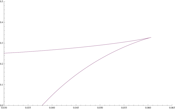
Figure 7: The $\frac{E}{T\sqrt{\lambda}}$ vs. $L$ plots of the transverse and longitudinal configurations at $\eta=0$. Even though the numerics that gives rise to the curves is different, the two are exactly on top of each other.

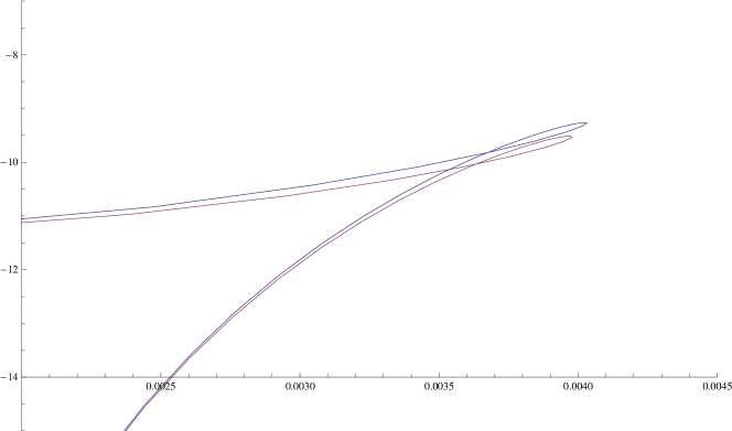
Figure 8: The $\frac{E}{T\sqrt{\lambda}}$ vs. $L$ plots for the two cases at $\eta=6$. The longitudinal curve is the one at higher energy. The qualitative features are identical at other values of $\eta\neq 0$.

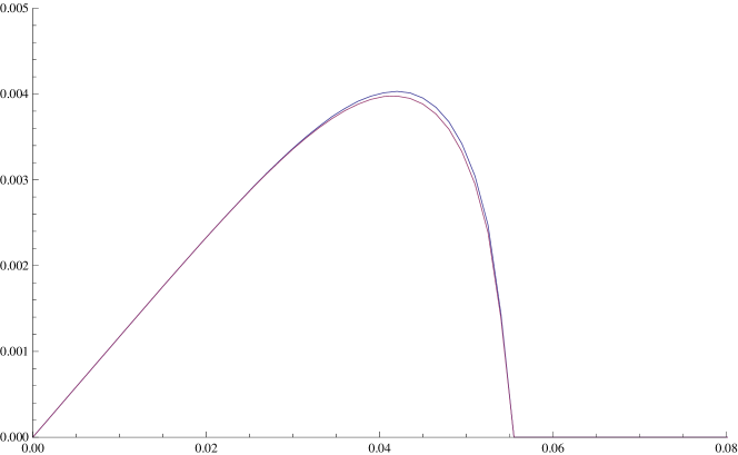
Figure 9: $LT$ vs. $\rho$ for $\eta=6$ for the two cases. The transverse case (II) is marginally lower, as expected from the intuition of figure 4 in [5].

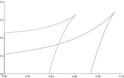
(a) $\eta$=0.

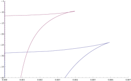
(b) $\eta=6$

Figure 10: Plots of $\frac{E}{T\sqrt{\lambda}}$ vs. $LT$ for baryons (lower curves) and dissociated configurations (upper curves). For less clutter we only show the transverse case.

Using the expressions from the previous subsections and the numerical simulations resulting from them, we can make comparisons between the energies of the two dissociated configurations. The curves are similar in both cases, except that the longitudinal quarks are at a higher energy when the windspeed is non-zero. The energy plots should be identical when the windspeed goes to zero since case I and II are identical in this case, so this can be used as a consistency check of our numerics. This is indeed what we find as clear from the $\eta=0$ plot. We show the plots of $E$ vs. $L$ for two representative cases ($\eta=0$ and $\eta=6$), in their interesting regimes of parameters. The fact that longitudinal configurations are at a higher energy than transverse ones has previously been observed in the case of mesonic configurations in [4] (see right panel of figure 6 in [4]).

Another observation one can make from the plots is that the energies of the dissociated configurations are always above those of the corresponding undissociated configurations for sufficiently large values of $\eta$, and this is shown in Figure 10b. This result is reasonable. The zero of the energy at each $\eta$ is set by the (colored) trailing string at that $\eta$. We also know from a previous section (see also [5]) that baryons have negative energy with respect to this datum, for sufficiently large windspeeds. So the configurations we are investigating here, which are morally between baryons and free strings, should naturally have intermediate energies. For small enough windspeed, there is some changes in these comparative plots, and we present them in Figure 10a. The cusp region is above zero energy even for the undissociated baryon in this case, as expected (see also [5]).

The structure of the energy curves for the dissociated cases is roughly

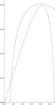
Figure 11: Typical shapes of $E$ and $L$ vs. $\rho$ for any $\eta$ and for any configuration. The axes have been re-scaled to fit the curves on the same plot, and the specific values are not to be paid attention to.

similar to that of the undissociated case, but in the plots here, we have zoomed in on the fine structure. The one significant difference with the baryonic case is that instead of a cusp, for non-zero boost, here we see a loop. We have done these numerical simulations for various configurations and various resolutions (see also Appendix C), so it seems very unlikely that this loop is a result of some systematic numerical error. The loops arise as a robust feature of all dragging configurations. In particular, they vanish for color non-singlet configurations only when the windspeed is zero and there is no drag (see Figure 7). The technical reason why the loops arise in E vs. L plots is not hard to see. The schematic plots of $E$ vs. $\rho$ and $L$ vs. $\rho$ for generic configurations and generic $\eta$ are given in the figure to the right. They both have one maximum, and for the case of non-drag configurations, the peaks in both $E$ and $L$ happen for the same value of $\rho$. But for dragging configurations, the peaks in $E$ are displaced to the left with respect to the peak in $L$, and therein lie the origins of the loop. It would be nice to understand the physical origins of this shift, better.

We suspect that these loops can be used as a measure of the drag of the configuration, because their areas seem to vary depending on the configurations. The fact that the loops have non-zero area for dragging configurations, and the fact that the area of the loop in the $\frac{E}{T\sqrt{\lambda}}$ vs. $LT$ plot has dimensions of energy in string units, suggests that this could perhaps be used as a measure of the energy loss. It would certainly be very interesting to study this further, and we plan to come back to this in the future.

4 Discussions and Loose Ends

We have already reported the main conclusions in the introduction, so here we will merely make some comments.

There are some natural extensions to the work done here. We have considered the special case of $N_{c}=4$ quarks, and found that we can reproduce and extend the results in the literature that deal with color singlet configurations. Considering a uniform distribution of quarks along the circle where the large $N_{c}$ limit is more systematic would be a natural next step. This will be more complicated because the strings are now not along the coordinate axes. More generic gauge theories, configurations other than circular baryons, more generic wind directions etc. are all possible lines of investigation, especially in understanding the possibility of extracting universal predictions valid across conformal/confining gauge theories.

In this paper, we have compared dissociated configurations which capture some aspects of the energetics of baryon dissociation. But it should be emphasized that the results of this paper are tentative. It would be nice to investigate other configurations, especially those with more quarks. Another interesting possibility is to do a scan of the various dissociation configurations at various angles and lengths. In particular, investigating other configurations which are identical except for their orientations would be useful.

Our original configuration of four quarks was specifically chosen to simplify the calculations. This is a perfectly good starting point, but it also suffers from the drawback that we cannot investigate many interesting configurations. A good example is the transverse and longitudinal configurations (analogous to the two configurations we investigated in section 3) after two quarks have dissociated. Both these configurations are not allowed because the force balance conditions on the D5-brane are too restrictive.

To get a full and unambiguous understanding of the possible dissociation patterns, we need a more exhaustive study of the various hints we have found in this paper. We have tried to stay close to the configurations which are most easily tractable. Our aim here has been to set up some of the framework and leave the more thorough work to a more elaborate future project, perhaps with more man-power. Some of these questions are currently under investigation.

5 Acknowledgments

It is a pleasure to thank Krishna Rajagopal for encouragement, clarifying correspondence and helpful comments on a previous version of the manuscript. I also thank Christina Athanasiou, Francesco Bigazzi, Stanislav Kuperstein and Carlo Maccaferri for discussions. This work is supported in part by IISN - Belgium (convention 4.4505.86), by the Belgian National Lottery, by the European Commission FP6 RTN programme MRTN-CT-2004-005104 in which the author is associated with V. U. Brussel, and by the Belgian Federal Science Policy Office through the Interuniversity Attraction Pole P5/27.

Appendix

A.  Equations of Motion

The equations governing the various static baryon-like configurations is obtained by varying the total action with respect to the string coordinates and with respect to the position of the D5-brane. Since the boundaries of the strings (at the D5-brane) are also supposed to be varying, one ends up getting a bit more than the usual Euler-Lagrange equations. The basic ideas are presented in [5], but we have chosen to redo it here for the case when there are dragging strings to clarify the origin of some negative signs which turn out to be crucial in this work.

The action for the system takes the general form

$$S=\sum_{m\in\{{\rm up}\}}\int_{r_{e}}^{\infty}{\cal L}_{m}(x_{i,m}^{\prime},r)dr+\sum_{n\in\{{\rm down}\}}\int_{r_{0}}^{r_{e}}{\cal L}_{n}(x_{i,n}^{\prime},r)dr+S_{D5}(r_{e}),$$ (A.1)

where we have denoted all the functional dependencies on the relevant variables. $x_{i,m}$ stands for the the $i$-th coordinate of string $m$. Primes are, again, with respect to $r$. The summation over the strings will be written explicitly in what follows, but the summation over $i$, should be understood from the context.

First we vary with respect to the $x$’s and get the individual equations of motion for the various strings. But since the boundaries are also allowed to vary, we also get boundary equations of motion which give further constraints on the configurations. Setting $\delta S=0$ (for variations of $x_{i}$), we end up with

$$0=\sum_{m\in\{{\rm up}\}}\int_{r_{e}}^{\infty}dr\frac{\partial{\cal L}_{m}}{\partial x_{i,m}^{\prime}}\delta x_{i,m}^{\prime}+\sum_{n\in\{{\rm down}\}}\int_{r_{0}}^{r_{e}}dr\frac{\partial{\cal L}_{n}}{\partial x_{i,n}^{\prime}}\delta x_{i,n}^{\prime}\hskip 65.04256pt$$ (A.2)

$$=\sum_{m\in\{{\rm up}\}}\int_{r_{e}}^{\infty}dr\biggl{[}\frac{d}{dr}\left(\frac{\partial{\cal L}_{m}}{\partial x_{i,m}^{\prime}}\delta x_{i,m}\right)-\frac{d}{dr}\left(\frac{\partial{\cal L}_{m}}{\partial x_{i,m}^{\prime}}\right)\delta x_{i,m}\biggr{]}+\sum_{n\in\{{\rm down}\}}\int_{r_{0}}^{r_{e}}dr\biggr{[}m\rightarrow n\biggl{]}.$$

We have written $\delta x_{i,m}^{\prime}$ as $d(\delta x_{i,m})/dr$ and done an integration by parts as usual. Since the variations $\delta x_{i}$ are arbitrary in the bulk (of the string), the second term in each piece has to be zero and gives rise to the standard Euler-Lagrange equations. In the present case they take the form:

$$\frac{\partial{\cal L}_{m}}{\partial x_{i,m}^{\prime}}={\rm const.}\equiv K_{i,m},\ \ \frac{\partial{\cal L}_{n}}{\partial x_{i,n}^{\prime}}={\rm const.}\equiv K_{i,n}.$$ (A.3)

What remains in the variation is

$$0=\sum_{m\in\{{\rm up}\}}\int_{r_{e}}^{\infty}dr\frac{d}{dr}\left(\frac{\partial{\cal L}_{m}}{\partial x_{i,m}^{\prime}}\delta x_{i,m}\right)+\sum_{n\in\{{\rm down}\}}\int_{r_{0}}^{r_{e}}dr\frac{d}{dr}\left(\frac{\partial{\cal L}_{n}}{\partial x_{i,n}^{\prime}}\delta x_{i,n}\right)$$

$$=-\sum_{m\in\{{\rm up}\}}\frac{\partial{\cal L}_{m}}{\partial x_{i,m}^{\prime}}\delta x_{i,m}\bigg{|}_{r=r_{e}}+\sum_{n\in\{{\rm down}\}}\frac{\partial{\cal L}_{n}}{\partial x_{i,n}^{\prime}}\delta x_{i,n}\bigg{|}_{r=r_{e}}\hskip 36.135pt$$ (A.4)

The strings are fixed at $r=r_{0}$ and $r=\infty$, so the terms from those ends of the integral don’t contribute. Also, at $r=r_{e}$, the strings are allowed to move, but only under the constraint that they are all still attached at the baryon vertex. This means that $\delta x_{i,m}|_{r_{e}}=\delta x_{i,n}|_{r_{e}}\equiv\delta x_{i}|_{r_{e}}$. Another input comes from the Euler-Lagrange equations above. They say, in particular, that $\frac{\partial{\cal L}}{\partial x_{i}^{\prime}}\big{|}_{r_{e}}=K_{i}$. Putting this all together, we end up with

$$\sum_{m\in\{{\rm up}\}}K_{i,m}-\sum_{n\in\{{\rm down}\}}K_{i,n}=0,$$ (A.5)

which gives rise to three equations, one for each $i$.

Now we turn to variations in $r_{e}$. The idea here is that we vary the boundary $r_{e}$, an look for variations in $x$ which result from considering the extrema of the action with this new boundary. In other words, in Figure 12, both $x$ and $\bar{x}$ are solutions of the Euler-Lagrange equations with their respective boundaries.

Figure 12: The classical solutions corresponding to different boundaries.

One way to handle this shift in boundary is to think of $r$ as a map from $u\in[0,1]$ to the integration range (i.e., write $r$ as $r(u)$). Then we can think of $u$ as the time variable, with fixed boundaries $0$ and $1$, and $r$ will be just another coordinate. The changes in the boundary can be re-interpreted now as variations in $r$, at the fixed boundaries of the $u$-interval. Thus we have translated a moving boundary to a boundary term: something easily handled using standard variational approaches (See e.g., chapter 1 of [24] for a clean discussion of variational methods with boundary terms.). This method works, but unfortunately our action involves different pieces which contain different ranges for $r$: the upward strings go from $r_{e}$ to $\infty$, while the downward strings are from $r_{0}$ to $r_{e}$. This makes this approach somewhat complicated, so we will follow another path which is much more direct and intuitive.

Let us consider what happens to the classical solutions of a system with the action

$$S_{0}=\int_{0}^{r_{e}}L\left(x(r),x^{\prime}(r)\right)dr,$$ (A.6)

under variations of the boundary. We are interested in finding new equations of “motion” by setting

$$0=\delta_{r_{e}}S_{0}=\int_{0}^{r_{e}+\delta r_{e}}L\left(\bar{x},\bar{x}^{\prime}\right)dr-\int_{0}^{r_{e}}L\left(x,x^{\prime}\right)dr$$ (A.7)

The important thing to note here is that $\bar{x}$ is supposed to be the classical solution corresponding to variations with the boundary fixed at $r_{e}+\delta r_{e}$, just as $x$ is the classical solution with boundary fixed at $r_{e}$. We have denoted $\bar{x}(r)-x(r)\equiv\delta x(r)$. Upto first order in small quantities, we can write,

$$0=\int_{0}^{r_{e}}\big{(}L(\bar{x},\bar{x}^{\prime})-L(x,x^{\prime})\big{)}dr+L(x,x^{\prime})|_{r_{e}}\delta r_{e}.$$ (A.8)

By the usual tricks, the first piece can be massaged into the form

$$\int_{0}^{r_{e}}dr\left(\frac{\partial L}{\partial x}\ \delta x+\frac{\partial L}{\partial x^{\prime}}\ \delta x^{\prime}\right)=\int_{0}^{r_{e}}dr\biggl{[}\left(\frac{\partial L}{\partial x}-\frac{d}{dr}\frac{\partial L}{\partial x^{\prime}}\right)\delta x+\frac{d}{dr}\left(\frac{\partial L}{\partial x^{\prime}}\ \delta x\right)\biggr{]}.$$

The Euler-Legrange term vanishes because $x$ is a classical path, and the other piece gets integrated and receives contributions only from the boundary. Since we imagine that the boundary at zero is held fixed, we end up with

$$0=\frac{\partial L}{\partial x^{\prime}}\ \delta x\bigg{|}_{r_{e}}+L(x,x^{\prime})|_{r_{e}}\delta r_{e}.$$ (A.9)

An important input at this stage comes from the fact that $\delta x(r)$ is the variation at fixed $r$ between classical solutions with different boundaries. Notice that by definition $\delta_{T}x(r_{e})=\delta x|_{r_{e}}+\frac{\partial x}{\partial r}\delta r\big{|}_{r_{e}}$ is zero: at the new boundary $r_{e}+\delta r_{e}$, the new classical solution ${\bar{x}}$ is supposed to have vanishing variations as well. So we get the final result,

$$0=\left(L-\frac{\partial L}{\partial x^{\prime}}x^{\prime}\right)\bigg{|}_{r_{e}}.$$ (A.10)

This was done for the case when the moving boundary was at the upper end of integration. For quarks hanging from the boundary of AdS, there will be an overall sign. Putting all these ingredients together, we finally get

$$-\sum_{m\in\{{\rm up}\}}\bigg{(}{\cal L}_{m}-\frac{\partial{\cal L}_{m}}{\partial x_{i,m}^{\prime}}x_{i,m}^{\prime}\bigg{)}\bigg{|}_{r=r_{e}}+\sum_{n\in\{{\rm down}\}}\bigg{(}{\cal L}_{n}-\frac{\partial{\cal L}_{n}}{\partial x_{i,n}^{\prime}}x_{i,n}^{\prime}\bigg{)}\bigg{|}_{r=r_{e}}+\frac{dS_{D5}}{dr_{e}}=0\hskip 14.45377pt$$ (A.11)

as the $r_{e}$-equation of motion for the various quarks and the D5-brane.

B.  Trailing String

In order to get a handle on the various dissociated baryonic configurations, we need to understand the trailing string solution that extends from the D5-brane to the black hole horizon. We will show in this appendix that the most general string of this form in the $x_{1}-x_{3}-r$ space lies along the wind direction ($x_{3}-r$ plane). This intuitively natural conclusion is important because (due to the force balance conditions at the D5 brane) it considerably restricts the resultant dissociation configurations that are allowed.

The action for the most general static string stretched between the D5 and the horizon is,

$$S=\frac{{\cal T}}{2\pi\alpha^{\prime}}\int_{r_{0}}^{r_{e}}dr\sqrt{A\Big{(}\frac{1}{f}+\frac{r^{2}x_{1}^{\prime 2}}{R^{2}}\Big{)}+\frac{r^{2}f(r)x_{3}^{\prime 2}}{R^{2}}}.$$ (B.12)

The equations of motion for the two components are

$$x_{1}^{\prime}=\frac{R^{2}}{r}\frac{K_{1}}{\sqrt{r^{2}fA-R^{2}K_{3}^{2}A-R^{2}K_{1}^{2}f}},$$ (B.13)

$$x_{3}^{\prime}=\frac{R^{2}}{fr}\frac{K_{3}A}{\sqrt{r^{2}fA-R^{2}K_{3}^{2}A-R^{2}K_{1}^{2}f}}.$$ (B.14)

By defining

$$t=\frac{r}{r_{0}},\ \ \mu=\frac{\alpha}{\rho^{2}},\ \ \nu=\frac{\beta}{\rho^{2}}\ \ {\rm and}\ \ x_{1,3}=\frac{R^{2}}{r_{0}}z_{1,3},$$ (B.15)

we can rewrite the above equations as

$$\left(\frac{dz_{1}}{dt}\right)^{2} = \mu^{2}\frac{1}{(t^{4}-\cosh^{2}\eta)(t^{4}-1-\nu^{2})-\mu^{2}(t^{4}-1)},$$ (B.16)

$$\left(\frac{dz_{3}}{dt}\right)^{2} = \frac{\nu^{2}\ (t^{4}-\cosh^{2}\eta)^{2}}{(t^{4}-1)^{2}}\frac{1}{(t^{4}-\cosh^{2}\eta)(t^{4}-1-\nu^{2})-\mu^{2}(t^{4}-1)}.$$ (B.17)

We would like to have simultaneous solutions of these two equations. A real solution can clearly only exist if

$$(t^{4}-\cosh^{2}\eta)(t^{4}-1-\nu^{2})-\mu^{2}(t^{4}-1)>0.$$ (B.18)

(We will be sloppy about distinguishing $>$ and $\geq$ in what follows, we will consider the boundaries explicitly.) The variable $t$ ranges from $t=1$ at $r=r_{0}$ (horizon) to $t=1/\rho$ at $r=r_{e}$ (D5 brane). We are interested in the case where $1/\rho>\sqrt{\cosh\eta}$ (See, for example, the screening length plots.). So for the entire range $1<t<\sqrt{\cosh\eta}+\epsilon$, with $\epsilon$ small enough and positive, the above inequality should hold for the solution to make sense. Doing a variable redefinition, this means that

$$x^{2}+x(\sinh^{2}\eta-\mu^{2}-\nu^{2})-\mu^{2}\sinh^{2}\eta>0,$$ (B.19)

should hold for $-\sinh^{2}\eta<x<\delta$ with small, positive $\delta$. The above inequality is satisfied as long as $x$ is either less or more than both the roots of the quadratic (the discriminant is positive, so the roots are never complex). If one of these ranges overlaps with $-\sinh^{2}\eta<x<\delta$, then we have a solution. This happens iff

$$-\sinh^{2}\eta>\frac{-(\sinh^{2}\eta-\mu^{2}-\nu^{2})+\sqrt{(\sinh^{2}\eta-\mu^{2}-\nu^{2})^{2}+4\mu^{2}\sinh^{2}\eta}}{2},$$ (B.20)

or

$$\delta<\frac{-(\sinh^{2}\eta-\mu^{2}-\nu^{2})-\sqrt{(\sinh^{2}\eta-\mu^{2}-\nu^{2})^{2}+4\mu^{2}\sinh^{2}\eta}}{2}.$$ (B.21)

The former inequality implies

$$\nu^{2}\sinh^{2}\eta<0.$$ (B.22)

This is clearly impossible, but there remains the possibility of the limiting case $\nu=0$, when the inequality is saturated. But this case is clearly pathological because it is easy to see that the original inequality (B.18) is violated for values of $t$ that lie close enough to 1. The remaining possibility is the second inequality (B.21). This can be rewritten as

$$\delta^{2}+\delta(\sinh^{2}\eta-\mu^{2}-\nu^{2})-\mu^{2}\sinh^{2}\eta>0,$$ (B.23)

and it needs to be satisfied if we tune $\delta$ small enough. This means that the only possibility is the limiting case $\mu=0$, where the inequality is saturated. But this is precisely the case when the trailing string is purely along $x_{3}$, which gives rise to the solution considered in appendix A of [4].

C.  Other Configurations

In this appendix we will look at some dissociated configurations to illustrate the fact that the energy plots can significantly differ from the ones considered before, depending on the configuration of quarks. The configurations we consider here are the minimal configurations allowed, if one stipulates that after a quark has dissociated, the remaining quarks in the baryon still remain on the circle. Of course, since we do not understand the dynamics, this is an ad hoc assumption. The purpose of this section is to give a flavor of the various dissociations patterns allowed.

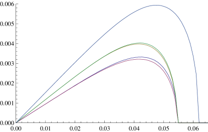
Figure 13: $LT$ vs. $\rho$ for the various cases. The top curve is for the undissociated baryon. The color code for the rest is as follows. Violet: case B, blue: case A, green: case I (from section 3), brown: case II. All the plots in this appendix are for $\eta=6$.

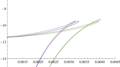
Figure 14: $\frac{E}{T\sqrt{\lambda}}$ vs. $L$ at $\eta=6$. The color code is the same as before.

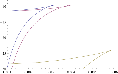
Figure 15: $\frac{E}{T\sqrt{\lambda}}$ vs. $L$ at $\eta=6$. The lowest curve is undissociated baryon, the rest of the color code is the same as before.

The configurations we consider are easily described by the condition that the quarks remain on the circle. The force balance conditions for our simple system are stringent enough that if the dissociated quark is one of the transverse ones, then not all of the remaining three quarks can remain in a circle. So we will look at the two cases where one of the quarks in the longitudinal direction is the dissociated one. In the $(x_{1},x_{3})$ plane, the two cases we consider will be defined by the quark positions

$${\rm Case\ A:} (1,0),(-1,0),(0,1),$$ (C.24)

$${\rm Case\ B:} (1,0),(-1,0),(0,-1).$$ (C.25)

For example, in this notation, the longitudinal case (case I) considered in the main text will be defined by the quark locations $(0,1),(0,0),(0,-1)$.

We will not present the details of the computations because the general formalism is the same as in the examples we considered in the main body of the paper. The one slight subtlety is that to make sure that the boundary quarks are arranged a circle, the relations we need to impose are,

$$L_{x_{3}}^{(2)}-L_{x_{3}}^{(1\ {\rm or}\ 3)}=L_{x_{1}}^{(1\ {\rm or}\ 3)}$$ (C.26)

for case A, and

$$L_{x_{3}}^{(1\ {\rm or}\ 3)}-L_{x_{3}}^{(2)}=L_{x_{1}}^{(1\ {\rm or}\ 3)},$$ (C.27)

for case B. The $L_{x_{i}}$ are measured from the D5-brane, and the superscripts denote the relevant quark (notice the $1\leftrightarrow 3$ symmetry). We present here the plots of the energies, screening lengths, together with those of the cases considered in section 3. The comparisons with the undissociated baryons are also presented.

References

- [1] J. M. Maldacena, The large N limit of superconformal field theories and supergravity, Adv. Theor. Math. Phys. 2, 231 (1998) [Int. J. Theor. Phys. 38, 1113 (1999)] [arXiv:hep-th/9711200]. E. Witten, Anti-de Sitter space and holography, Adv. Theor. Math. Phys. 2, 253 (1998) [arXiv:hep-th/9802150]. S. S. Gubser, I. R. Klebanov and A. M. Polyakov, Gauge theory correlators from non-critical string theory, Phys. Lett. B 428, 105 (1998) [arXiv:hep-th/9802109]. O. Aharony, S. S. Gubser, J. M. Maldacena, H. Ooguri and Y. Oz, Large N field theories, string theory and gravity, Phys. Rept. 323, 183 (2000) [arXiv:hep-th/9905111]. S. J. Rey and J. T. Yee, Macroscopic strings as heavy quarks in large N gauge theory and anti-de Sitter supergravity, Eur. Phys. J. C 22, 379 (2001) [arXiv:hep-th/9803001]. Wilson loops in large N field theories, Phys. Rev. Lett. 80, 4859 (1998) [arXiv:hep-th/9803002]. S. J. Rey, S. Theisen and J. T. Yee, Wilson-Polyakov loop at finite temperature in large N gauge theory and anti-de Sitter supergravity, Nucl. Phys. B 527, 171 (1998) [arXiv:hep-th/9803135]. A. Brandhuber, N. Itzhaki, J. Sonnenschein and S. Yankielowicz, Wilson loops in the large N limit at finite temperature, Phys. Lett. B 434, 36 (1998) [arXiv:hep-th/9803137].
- [2] H. Liu, K. Rajagopal and U. A. Wiedemann, An AdS/CFT calculation of screening in a hot wind, Phys. Rev. Lett. 98, 182301 (2007) [arXiv:hep-ph/0607062].
- [3] E. Caceres, M. Natsuume and T. Okamura, Screening length in plasma winds, JHEP 0610, 011 (2006) [arXiv:hep-th/0607233].
- [4] H. Liu, K. Rajagopal and U. A. Wiedemann, Wilson loops in heavy ion collisions and their calculation in AdS/CFT, JHEP 0703, 066 (2007) [arXiv:hep-ph/0612168].
- [5] C. Athanasiou, H. Liu and K. Rajagopal, Velocity Dependence of Baryon Screening in a Hot Strongly Coupled Plasma, arXiv:0801.1117 [hep-th].
- [6] E. Witten, Baryons and branes in anti de Sitter space, JHEP 9807, 006 (1998) [arXiv:hep-th/9805112]. A. Brandhuber, N. Itzhaki, J. Sonnenschein and S. Yankielowicz, Baryons from supergravity, JHEP 9807, 020 (1998) [arXiv:hep-th/9806158].
- [7] E. Witten, Anti-de Sitter space, thermal phase transition, and confinement in gauge theories, Adv. Theor. Math. Phys. 2, 505 (1998) [arXiv:hep-th/9803131].
- [8] K. Peeters, J. Sonnenschein and M. Zamaklar, Holographic melting and related properties of mesons in a quark gluon plasma, Phys. Rev. D 74, 106008 (2006) [arXiv:hep-th/0606195].
- [9] M. Chernicoff, J. A. Garcia and A. Guijosa, The energy of a moving quark-antiquark pair in an N = 4 SYM plasma, JHEP 0609, 068 (2006) [arXiv:hep-th/0607089].
- [10] M. Chernicoff and A. Guijosa, Energy loss of gluons, baryons and k-quarks in an N = 4 SYM plasma, JHEP 0702, 084 (2007) [arXiv:hep-th/0611155].
- [11] C. P. Herzog, A. Karch, P. Kovtun, C. Kozcaz and L. G. Yaffe, Energy loss of a heavy quark moving through N = 4 supersymmetric Yang-Mills plasma, JHEP 0607, 013 (2006) [arXiv:hep-th/0605158].
- [12] S. S. Gubser, Drag force in AdS/CFT, Phys. Rev. D 74, 126005 (2006) [arXiv:hep-th/0605182].
- [13] C. P. Herzog, Energy loss of heavy quarks from asymptotically AdS geometries, JHEP 0609, 032 (2006) [arXiv:hep-th/0605191].
- [14] J. J. Friess, S. S. Gubser and G. Michalogiorgakis, Dissipation from a heavy quark moving through N = 4 super-Yang-Mills plasma, JHEP 0609, 072 (2006) [arXiv:hep-th/0605292].
- [15] M. Li, Y. Zhou and P. Pu, High spin baryon in hot strongly coupled plasma, arXiv:0805.1611 [hep-th].
- [16] K. Sfetsos and K. Siampos, Stability issues with baryons in AdS/CFT, JHEP 0808, 071 (2008) [arXiv:0807.0236 [hep-th]].
- [17] S. D. Avramis, K. Sfetsos and D. Zoakos, On the velocity and chemical-potential dependence of the heavy-quark interaction in N = 4 SYM plasmas, Phys. Rev. D 75, 025009 (2007) [arXiv:hep-th/0609079].
- [18] A. Karch and E. Katz, Adding flavor to AdS/CFT, JHEP 0206, 043 (2002) [arXiv:hep-th/0205236].
- [19] J. Babington, J. Erdmenger, N. J. Evans, Z. Guralnik and I. Kirsch, Chiral symmetry breaking and pions in non-supersymmetric gauge / gravity duals, Phys. Rev. D 69, 066007 (2004) [arXiv:hep-th/0306018].
- [20] M. Kruczenski, D. Mateos, R. C. Myers and D. J. Winters, Towards a holographic dual of large-N(c) QCD, JHEP 0405, 041 (2004) [arXiv:hep-th/0311270].
- [21] K. Ghoroku and M. Ishihara, Baryons with D5 Brane Vertex and k-Quarks, Phys. Rev. D 77, 086003 (2008) [arXiv:0801.4216 [hep-th]].
- [22] K. Ghoroku, M. Ishihara, A. Nakamura and F. Toyoda, Multi-quark baryons and color screening at finite temperature, arXiv:0806.0195 [hep-th].
- [23] O. Kaczmarek and F. Zantow, Static quark anti-quark interactions in zero and finite temperature QCD. I: Heavy quark free energies, running coupling and quarkonium binding, Phys. Rev. D 71, 114510 (2005) [arXiv:hep-lat/0503017].
- [24] W. Dittrich and M. Reuter, “Classical and Quantum Dynamics: From Classical Paths to Path Integrals”, Springer, 2001, 385 p.