Tailoring PDC speckle structure.

Abstract

Speckle structure of parametric down conversion light has recently received a large attention due to relevance in view of applications to quantum imaging

The possibility of tailoring the speckle size by acting on the pump properties is an interesting tool for the applications to quantum imaging and in particular to the detection of weak object under shot-noise limit.

Here we present a systematic detailed experimental study of the speckle structure produced in type II PDC with particular attention to its variation with pump beam properties.

1 Introduction

Thermal or pseudothermal light (as the one obtained by scattering of coherent light by a diffuser) presents a random intensity distribution known as speckle pattern [2]. This structure can have interesting applications, e.g. in metrology [3].

In particular, speckle structure of parametric down conversion (PDC) light has recently received a large attention due to relevance in view of applications to quantum imaging [4].

The aim of Sub Shot Noise (SSN) quantum imaging is to obtain the image of a weak absorbing object with a level of noise below the minimum threshold that is unavoidable in the classical framework of light detection. Being interested in measuring an image, one is forced to consider a multi-mode source, which is able to display quantum correlation also in the spatial domain. Theoretically, this goal can be achieved by exploiting the quantum correlation in the photon number between symmetrical modes of SPDC . Typically the far field emission is collected by a high quantum efficiency CCD camera. It is fundamental to set the dimension of the modes coherence areas with respect to the dimension of the pixels. In particular, the single pixel dimension must be of the same order of magnitude of the coherence area or bigger, in order to fulfill the sub-shot noise correlation condition, compatibly with the requirement of large photon number operation. Thus, the possibility of tailoring the speckle size by acting on the intensity and size of the pump beam represents an interesting tool for the applications to quantum imaging and in particular to the detection of weak objects under shot-noise limit [4, 7, 6, 8].

A detailed theory of correlations and speckle structure in PDC has been developed in [5] and, in another regime, in [9] Furthermore, experimental results were presented in [6].

Nevertheless, a systematic comparison of experimental variation of speckle size and their correlations with the theoretical results of [5] is still missing.

In this paper we present a systematic detailed experimental study of the speckle structure produced in type II PDC with particular attention to its variation with pump beam properties. In particular dependence on pump power and size are investigated in detail: results that will represent a test bench for the theoretical models.

2 Theory

The process of SPDC is particularly suitable for studying the spatial quantum correlations [11], because it takes place with a large bandwidth in the spatial frequency domain. Any pair of transverse modes of the radiation (usually dubbed idler and signal), characterized by two opposite transverse momenta $\mathbf{q}$ and $-\mathbf{q}$, are correlated in the photon number, i.e. they contain, in an ideal situation, the same number of photons. In the far field zone, the single transverse mode is characterized by a coherence area, namely the uncertainty on the emission angle $\vartheta$ ($\tan\vartheta=\lambda q/2\pi$, $\lambda$ being the wavelength) of the twin photons. It derives from two effects that participate in the relaxation of the phase matching condition. On the one side the finite transverse dimension of the gain area inside the crystal, coinciding with the pump radius $w_{p}$ at low parametric gain. On the other side the finite longitudinal dimension of the system, i.e. along the pump propagation direction, that is generally given by the crystal length $l$.

The appearance of the emission is a speckled structure in which the speckles have, roughly, the dimension of the coherence area and for any speckle at position $\mathbf{q}$ there exists a symmetrical one in $-\mathbf{q}$ with equal intensity. This is rather evident in the ccd images of SPDC shown in Fig. 1.

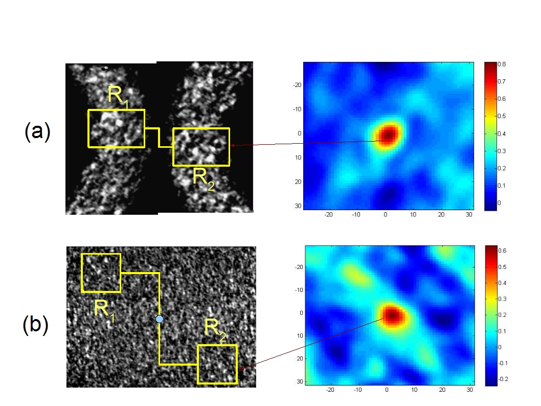
Figure 1: CCD’s images of the speckled structure of the type II PDC emission from a BBO non-linear crystal. The two partial rings in (a) represent the two correlated beams 1 and 2, selected by a narrow filter (Bandwidth=10 nm) around the degeneracy ($\omega_{1}=\omega_{2}=\omega_{p}/2$), whereas in (b) no filtering is applied. On the right hand site, are shown the respective cross-correlation functions, evaluated by fixing a region $R_{1}$ in the signal field and moving a region $R_{2}$ in the idler field. A point in the cross-correlation graph correspond to the correlation coefficient between $R_{1}$ and $R_{2}$ for a single position of $R_{2}$. The axes report the pixel by pixel displacement of region $R_{2}$.

In the following we summarize, very briefly, some elements of the theory describing this structure.

Omitting some unessential constants, the Hamiltonian describing the three fields parametric interaction is

$$\widehat{H}_{I}(t)\propto\int_{\mathcal{V}}\chi^{(2)}\;\widehat{\mathbf{E}}^{(+)}_{1}(\mathbf{r},t)\;\widehat{\mathbf{E}}^{(+)}_{2}(\mathbf{r},t)\;\widehat{\mathbf{E}}^{(-)}_{p}(\mathbf{r},t)\;d^{3}r+h.c$$ (1)

The evolution of the quantum system guided by Hamiltonian (1), in the case of relatively high gain regime and non-plane-wave pump, requires a numerical solution and it is discussed in detail in [5]. Anyway, in the low gain regime an analytical solution is achievable [13, 12]. Therefore, it is worth to briefly mention the result in the first order of the perturbation theory ($g\ll 1$) for a gaussian pump, where the quantum state of the scattered light has the entangled form

$$\left|\psi\right\rangle = \left|\mathrm{vac}\right\rangle+\exp\left[-\frac{i}{\hbar}\int\widehat{H}_{I}dt\right]\left|0\right\rangle$$ (2)

$$= \left|\mathrm{vac}\right\rangle+\sum_{\mathbf{q}_{1},\mathbf{q}_{2}}\sum_{\Omega}F(\mathbf{q}_{1},\mathbf{q}_{2},\Omega)\left|1_{\mathbf{q}_{1},\Omega}\right\rangle\left|1_{\mathbf{q}_{2},-\Omega}\right\rangle,$$

$$F(\mathbf{q}_{1},\mathbf{q}_{2},\Omega) = g\cdot\,\mathrm{sinc}\left[\frac{\Delta k(\mathbf{q}_{1},\mathbf{q}_{2},\Omega)\cdot l}{2}\right]e^{-(\mathbf{q}_{1}+\mathbf{q}_{2})^{2}\frac{w_{p}^{2}}{4}},$$ (3)

$$\omega_{1}=\omega_{p}/2+\Omega,\qquad\omega_{2}=\omega_{p}/2-\Omega.$$

$\mathbf{q}_{1,2}$ being the transverse wave vectors and $\omega_{p},\omega_{1},\omega_{2}$ the pump, idler and signal frequencies respectively. The coherence area, in the limit of low parametric gain $g$, can be estimated by the angular structure of the coincidence probability $\left|F(\mathbf{q}_{1},\mathbf{q}_{2})\right|^{2}$ at some fixed frequency $\Omega$. As mentioned before, now is clear that we deal with two functions that enter in the shaping of the coherence area: the $sinc$ function and the Fourier transformed gaussian pump profile. Since they are multiplied, the narrower determines the dimension of the area. The Half Width Half Maximum of the gaussian function, appearing in (3), is $\delta q=\sqrt{2\ln(2)}/w_{p}$. If we expand the longitudinal wave detuning around the exact matching point $\Delta k(\mathbf{q}_{0},\mathbf{q}_{0},\Omega)$, the linear part [12] dominates for angles $\vartheta_{0}(\mathbf{q}_{0})$, not too next to collinear regime and the $sinc$ function turns out to have a HWHM of $\Delta q=2,78/(l\tan\vartheta_{0})$ at degeneracy. On the other hand, around the collinear emission, the quadratic term prevails [5] and the bandwidth becomes $\Delta q=2,78*(2\pi/\lambda l)^{1/2}$. Concerning our experiment, we consider small (but not zero) emission angles $\vartheta$ and large enough pump radius $w_{p}$, such that we always work in the region $\delta q/\Delta q<1$. Therefore, in principle, the dimension of the coherence area is only determined by the pump waist.

When moving to higher gain regime, which is of greater interest for our experiment, the number of photon pairs generated in the single mode increases exponentially as $\propto\sinh^{2}(g)$ i.e. a large number of photons is emitted in the coherence time along the direction $\vartheta$. In this case, also the pump amplitude becomes important in the determination of the speckles dimension. As described in [7], this can be explained by a qualitative argumentation: inside the crystal, the cascading effect that causes the exponential growth of the number of generated photons is enhanced in the region where the pump field takes its highest value, i.e. close to the center of the beam. Thus, in high gain regime, most of the photon pairs are produced where the pump field is closed to its peak value. As a result the effective region of amplification inside the crystal becomes narrower than the beam profile. Thus, in the far field one should consider the speckles as the Fourier transform of the effective gain profile, that being narrower, produces larger speckles.

A further fundamental consideration for the practical implementation is that in high gain regime, instead of measuring the coincidences between two photons by means of two single photo-detectors, one collects a large portion of the emission by using for instance a CCD array with a certain fixed exposure time. Within this time several photons are collected by the single pixels and the result is an intensity pattern, having the spatial resolution of the pixel. Looking at the images, we can appreciate the speckled structure and a certain level of correlation of the speckles intensity between the signal and idler arms (Fig. 1(a) and (b)). We can define also the auto-correlation function of the signal intensity pattern itself, since in the single transverse mode of the signal arm there are many photons. To be precise the speckle’s dimension is better related to the spread of this function, although the two functions, the cross- and the auto- correlation, present in the very high gain regime the same behaviour with respect to the pump parameters, see [5].

From the experimental view-point it is convenient to study the auto-correlation because of the higher visibility that allows a more accurate estimation of its size.

3 Experiment

Our setup is depicted in Fig. 3. A type II BBO non-linear crystal ($l=1$ cm) is pumped by the third harmonic (wavelength of 355 nm ) of a Q-switched Nd:Yag laser. The pulses have a duration of 5ns with a repetition rate of 10 Hz and a maximum energy, at the selected wavelength, of about 200 mJ. The pump beam crosses a spatial filter (a lens with $f$=50 cm and an iris of 250 $\mu$m of diameter), in order to eliminate the non-gaussian components (see fig. 2). Before entering the crystal the pump is collimated and its diameter is varied, when necessary, by changing the distance between two lenses (a biconvex and a biconcave) placed after the spatial filter. After the crystal, the pump is stopped by a UV mirror, transparent to the visible (T=87% measured at 685nm), and by a low frequency-pass filter. The down converted photons (signal and idler) pass through a lens of 5 cm of diameter ($f=10$ cm) and an interference filter centered at the degeneracy $\lambda$=710 nm (10nm bandwidth) and finally measured by a CCD camera. We used a $1340X400$ CCD array, Princeton Pixis:400BR (pixel size of 20 $\mu$m), with high quantum efficiency (80%) and low noise ($\Delta=4$ electrons/pixel). The far field is observed at the focal plane of the lens in a $f-f$ optical configuration, that ensures that we image the Fourier transform of the crystal exit surface. Therefore a single transverse wavevector $\mathbf{q}$ is associated to a single point $\mathbf{x}=(\lambda f/2\pi)\mathbf{q}$ in the detection plane. The CCD acquisition time is set to 90 ms, so that each frame corresponds to the PDC generated by a single shot of the laser.

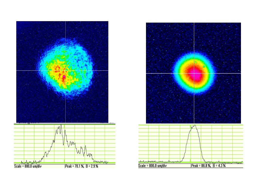
Figure 2: Image of the pump beam before (on the left) and after (on the right) spatial filtering.

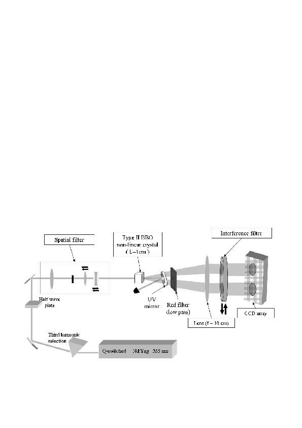
Figure 3: Experimental setup. A triplicated Nd-Yag laser beam, after spatial filtering, produces type II PDC in a BBO crystal, which is then measured, after an interference filter and pump elimination, by a CCD camera.

Let us define $N_{R}(\mathbf{x})$ the intensity level, proportional to the number of photons, registered by the pixel in the position $\mathbf{x}$ of a region $R$. $\delta N_{R}(\mathbf{x})=N_{R}(\mathbf{x})-\langle N_{R}(\mathbf{x})\rangle$ is the fluctuation around the mean value that is estimated as $\langle N_{R}(\mathbf{x})\rangle=(1/n)\sum_{\mathbf{x}}N_{R}(\mathbf{x})$, with $n$ the number of pixels. We evaluate the normalized spatial auto-correlations of the intensity fluctuations by choosing a large arbitrary region $R$, belonging for instance to the signal portion of the image, and measuring

$$C(\mathbf{\xi})=\frac{\left\langle\delta N_{R}(\mathbf{x})\delta N_{R}(\mathbf{x+\xi})\right\rangle}{\sqrt{\left\langle\delta N_{R}(\mathbf{x})^{2}\right\rangle\left\langle\delta N_{R}(\mathbf{x+\xi})^{2}\right\rangle}}.$$ (4)

where $\xi$ is the displacement vector in the pixel space and assumes discrete values. $C(\mathbf{\xi})$ has unit value for $\mathbf{\xi}=0$.

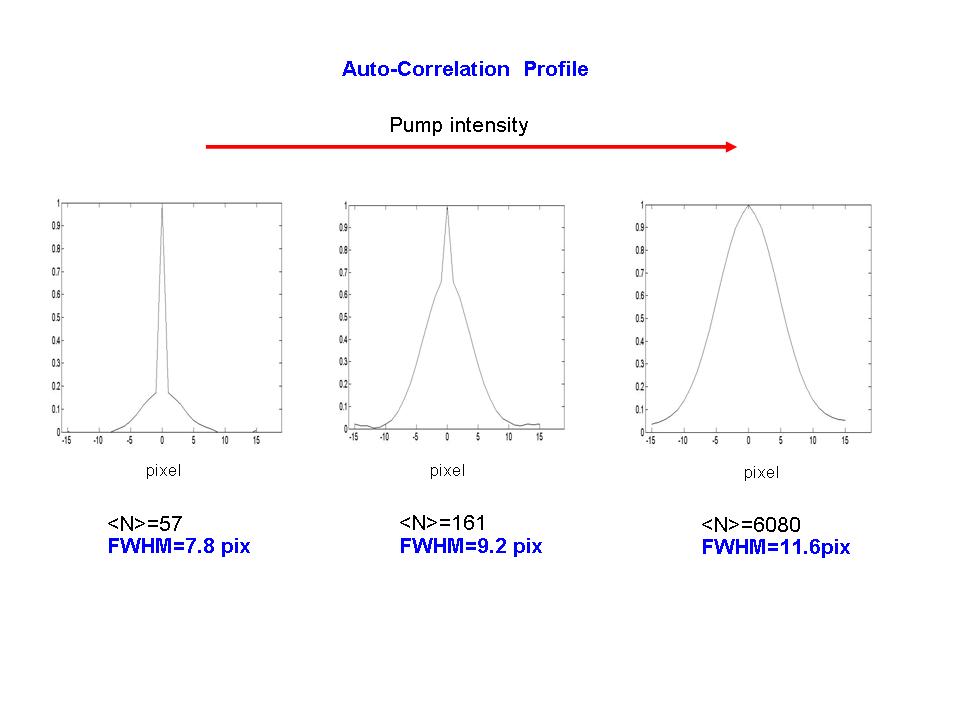
Figure 4: Section of the two dimensional auto-correlation function evaluated in single shot images at different pump intensity

Fig. 4 shows some typical section of the auto-correlation for different value of the pump intensity. One note that, especially for small photon number, the auto-correlation is dominated by the peak at $\mathbf{\xi}=0$ and drop down even for displacement of one pixel, creating symmetrically a sort of shoulder. This is explained by the presence of noise at the scale of the pixel: first of all the shot-noise that gives a contribution of $\langle N_{R}(\mathbf{x})\rangle$, then the electronic noise in the read-out and digitalization process is $\Delta$ and, finally, the quantum efficiency that fluctuates with a standard deviation $\delta\eta=3\%$ (we evaluated it using a self-calibration procedure similar to the one described in [14]). On the other side the fluctuations at the scale of the coherence area of the light are given by $\langle N_{R}(\mathbf{x})\rangle^{2}/M$, where $M$ is the number of modes (spatial modes $*$ temporal modes), collected by one pixel. Therefore a large number of spatial modes limits the visibility of the genuine auto-correlation of the field with respect to the other sources of noise due to the detection by CCD. Anyway we can take the width of the shoulder as the most correct estimation of the coherence radius. Fig. 5 reports on the left hand side, one of our main results, namely the speckle’s radius $R_{coh}$ as a function of the photon number per pixel for two different pump size $w_{p}=1.0$ mm and $w_{p}=0.7$ mm. The increasing of the radius of the auto-correlation function versus the mean number of photons can not be explained by the theory in the low gain regime, predicting no dependence on the gain, i.e. on the pump intensity. This is a signature of the fact that we are working in a non linear regime of PDC in which the parametric gain $g$ does not fulfill the condition $g\ll 1$, as we will discuss in the next paragraph. It must be noticed that we are constrained in the range of intensities of the pump. For high intensities we are limited by the damage threshold of optical components, for low intensities by the visibility of the speckle structure because we collect a lot of temporal modes in the same frame.

In order to comment the behavior of the radius it is important to evaluate the effective gain region. We adopt two approaches. First we try to evaluate $g$ by the statistics of the light. Approximatively, according to Fig. 5, we can consider the dimension of the pixel always smaller than the coherence area and thus the number of collected spatial modes $\sim 1$ [15]. We evaluate the number of temporal modes $M$, within this approximation, by using the property of the thermal statistics corrected for the presence of experimental imperfections described above:

$$\langle\delta^{2}N\rangle=\langle N\rangle+\frac{\langle N\rangle^{2}}{M}+\delta^{2}\eta\langle N\rangle^{2}+\Delta^{2}$$ (5)

The estimation is performed on a statistical ensemble of independent pixel belonging to a single shot frame, thus is definitely a spatial statistics.

After that, we can approximatively estimate the parametric gain by the relation

$$\langle N\rangle=\eta\cdot\eta_{coll}\cdot M\cdot\sinh^{2}(g),$$ (6)

where $\sinh^{2}(g)$ is the number of photons in the single space-temporal mode, $\eta$ is the quantum efficiency (including losses) and $\eta_{coll}$ is the collection efficiency. It takes into account that the pixel collects only a portion of the spatial mode and roughly is given by the ratio between the pixel area and the auto-correlation area $\eta_{coll}\approx A_{pix}/A_{coh}$. The result is reported in Fig. 5, on the right hand side. As expected, the gain $g$ is larger than $1$, confirming that we are working in high gain regime. Let also notice that, although each point is an average over tens of images they are distributed rather noisy, as well as the radius (on the left insert).

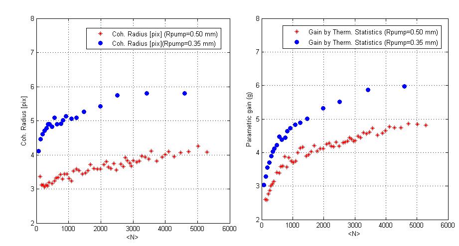
Figure 5: On the left, speckle’s radius and, on the right, parametric gain estimation, both as function of photon number per pixel, for two pump radii

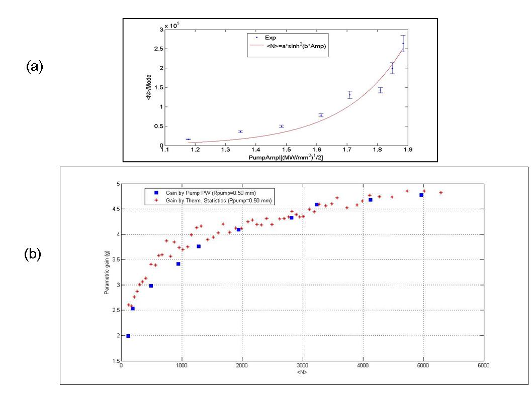
Figure 6: (a) Number of photons in a single mode as function of pump amplitude (b) Parametric gain as function of the photon number per pixel estimated from (a) and from the property of the thermal statistics

In order to explain the main features of the data it is fundamental to take into account the characteristics of the pump. It is the third harmonic of a multimode high power laser and the power is varied by the delay between the Q-switch turn-on and the lamp flash. The calibration curve delay-power (mean pulse power) has been measured by a power meter, and we observed a reproducibility with uncertainty around 10%. The fluctuation of the mean pulse power is about 20% (measured by a photodiode). Since the mean number of photons is proportional to $\sinh^{2}(g)$, the fluctuations of the pump power generate large fluctuations in the photons number from frame-to-frame.

Furthermore, a multimode laser when the number of modes $n$ is larger than few units should present a thermal statistics of the intensity fluctuation according to the formula $\delta I/I=\sqrt{1-1/n}$ [15] and, after the non linear process of second and third harmonic generation the fluctuations can increase even more. The expected temporal profile of the output pulse is very far from a smooth gaussian function. Therefore, taken into account the strong non-linearity of the PDC generation, it is reasonable to consider that, inside the single pulse entering the crystal, only few peaks of intensity contribute to the large majority of the PDC emission. The main consequence is that the number of effective temporal modes $M$, collected in the single shot, is much less than what expected by evaluating the ratio between the pulse duration (5 ns) and the PDC coherence time $\tau_{p}\sim 1$ ps and $M$ also fluctuates randomly from image to image. By using Eq. 5, we obtain a mean number of effective temporal modes $\overline{M}=170\pm 80$ when $w_{p}=1.0$ mm and $\overline{M}=60\pm 40$ for $w_{p}=0.7$ mm. At the same time, the values of the parametric gain $g$ are in general bigger than 1 (see Fig 5). The gain region in which we are working ensures the possibility to reach a sufficient non-linear cascading effect in the photon pairs production inside the crystal.

As a confirmation of the high non-linearity obtained in our experiment we estimate the gain $g$ in an independent way [16]. In Fig. 6(a) we present the measurement of the number of photon in the spatial mode defined as $\langle N_{mode}\rangle=\langle N\rangle\cdot A_{coh}$ by varying the mean pump amplitude $A_{pump}$, while the pump size is fixed to $w_{p}=1.0$ mm. Here the mean pump amplitude is the square root of the average power of the single pulse divide by the transverse pump area measured by a CCD. The data are fitted by the equation $\langle N_{R}\rangle=k\cdot\sinh^{2}(\sigma A_{pump})$, where $k$ is fixed to $k=\eta\overline{M}$, while $\sigma$ ($\sigma A_{pump}=g$) is the free parameter. The experimental values, mediated on three different acquisitions, are $\sigma=2.53\pm 0.04[\mathrm{mm^{2}/W}]^{1/2}$. Fig. 6(b) shows the comparison between the values of the gain obtained in this way (green squares) and in the previous statistical approach (the red dots). The data are very close, and we can conclude that we are actually in a strong non linear regime.

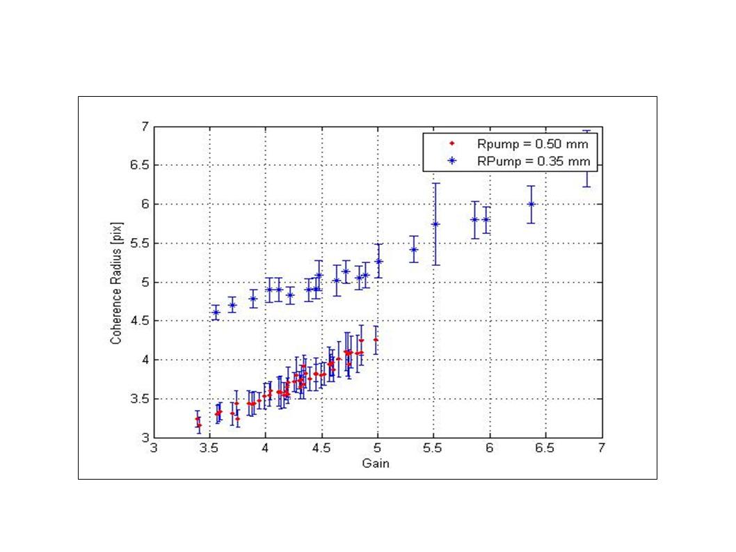
Figure 7: Coherence radius as function of the parametric gain

Now, let us consider the trend of the coherence radius versus the parametric gain for the two different pump size as reported in Fig. 7. The data are well fitted by two straight lines (not showed in figure), $R_{i}(g)=\alpha_{i}g+R_{i}(0)$ with $i=1,2$. We obtain that $\alpha_{1}(0.67\pm 0.06)$ and $\alpha_{2}(0.55\pm 0.06)$ agree within the their uncertainty. Although a comparison with a theoretical model in high gain regime is needed for a proper interpretation of our data, we can consider this behavior as an evidence of the influence of the gain and of the pump diameter on the dimension of the speckles. In fact, for the same value of the gain, the speckles radius is always larger when the pump size is smaller as predicted in the low gain.

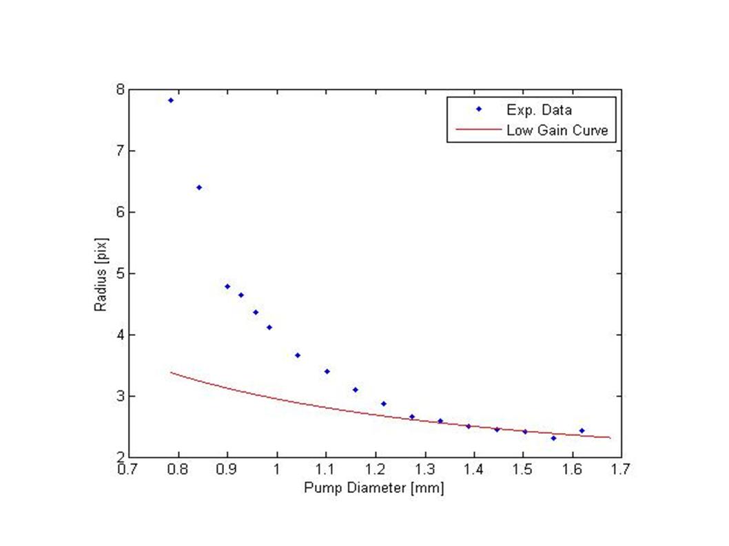
Figure 8: Observed dependence of the radius (in pixels) of the speckles from the pump diameter

Finally, we investigate the dependence of the radius of the speckles from the pump diameter, as shown in figure 8. We fix the power of the laser to 0,78 MW, within the fluctuations, and we change the diameter varying the distance between the two collimating lenses (see figure 3). Since the diameter changes, the intensity and the gain $g$ change as well. The theory, in low gain regime, provides that the radius of the speckles is proportional to the inverse of the pump size ($w_{p}$) obtaining the red line in figure. It approach the experimental data only when the pump diameter is large. This confirms the role of the high gain regime in the speckle size. In fact, together with the reduction of the pump diameter, the gain increases, and thus the effective gain area is even more reduced. This effect impresses upon the speckles size a stronger dependence with respect to the pump size.

4 Conclusion

This paper provides a detailed experimental study of the size of the coherence area in PDC in the high gain regime. We show that the speckles present, not only a dependence on the pump diameter, as in the usual low gain regime, but also a strong dependence form the pump intensity. The understanding of the behavior of the coherence area in the high gain regime is fundamental for the innovative application in the field of quantum imaging. Our results provide the basis for a comparison with the theoretical models; in general, the observed dependencies of speckles size on pump parameters allow the tailoring of speckles properties, an instrument useful not only for applications to quantum imaging but also for quantum metrology, quantum information, etc.

4.1 Acknowledgments

This work has been supported by MIUR (PRIN 2005023443-002), by 07-02-91581-ASP, by Regione Piemonte (E14) and by Fondazione Compagnia di San Paolo. Thanks are due to Alessandra Gatti, Enrico Brambilla, Lucia Caspani, Luigi Lugiato and Ottavia Jedrkiewicz for useful discussions.

References

- [1]
- [2] Goodman, J.W., Laser speckle and Related Phenomena ; Springer Verlag: Berlin, 1984.
- [3] Uno, K.; Uozumi, J.; Asakura, T. , Opt. Comm. 1996, 124, 16-22; Uozumi, J.; Ibrahim, M.; Asakura, T. Opt. Comm. 1998, 156, 350-358; Funamizu, H.; Uozumi, J. Journ. Mod. Opt. 2007, 54(10), 1511-1528.
- [4] Kolobov, M.I. editor Quantum Imaging Springer, New York, 2007.
- [5] Brambilla, E.; Gatti, A.; Bache, M.; Lugiato, L. A. Phys. Rev. A 2004, 69, 023802-1-6; Brambilla, E.; Gatti, A.; Lugiato, L. A.; Kolobov, M.I. Eur. Phys. J. D 2001, 15 127-135.
- [6] Jedrkiewicz, O.; Jang, Y. -K.; Brambilla, E.; Gatti, A.; Bache, M.; Lugiato, L. A.; Di Trapani, P. Phys. Rev. Lett. 2004, 93 , 243601-1-4; Jedrkiewicz, O.; Brambilla, E.; Bache, M.; Gatti, A.; Lugiato, L. A.; Di Trapani, P. Journal of Modern Optics 2006, 53, 575-595; Brida G.; Genovese M.; Meda A.; Ruo-Berchera, I. arXiv:0810.1470v1 [quant-ph].
- [7] Brambilla, E.; Caspani, L.; Jedrkiewicz, O.; Lugiato, L. A.; Gatti, A. Phys. Rev. A 2007, 77, 053807-1-6.
- [8] Bondani, M.; Allevi, A.; Zambra, G.; Paris, M. G. A.; Andreoni, A. Phys. Rev. A 2007, 76, 013833-1-5.
- [9] Allevi, A.; Bondani, M.; Ferraro, A.; Paris, M. G. A. Las. Phys. 2006, 16, 1451-1477.
- [10] Degiovanni, I.P.; Bondani, M.; Puddu, E.; Andreoni, A.; Paris, M. G. A. Phys. Rev A 2007, 76, 062309-1-9.
- [11] Genovese, M. Physics Reports, 2005, 413(6).
- [12] Burlakov, A.V.; Chekhova, M. V.; Klyshko, D. N.; Kulik, S. P.; Penin, A. N.; Shih, Y. H.; Strekalov, D. V. Phys. Rev. A 1997, 56, 3214-3225;
- [13] Klyshko, D.N. ”Photons and Nonlinear Optics”, Gordon and Breach Science Publishers, 1988; Pittman, T.B.; Strekalov, D. V.; Klyshko, D. N.; Rubin, M. H.; Sergienko, A. V.; Shih, Y. H. Phys. Rev. A 1996, 53, 2804-2815; Monken, C.H.; Souto Ribeiro, P. H.; Padua, S. Phys. Rev. A 1998, 57, 3123-3126; Fedorov, M.V.; Efremov, M. A.; Volkov, P. A.; Moreva, E. V.; Straupe, S. S.; Kulik, S. P. Phys. Rev. Lett. 2007, 99, 063901-1-4.
- [14] Jiang, Y.; Jedrkiewicz, O.; Minardi, S.; Di Trapani, P.; Mosset, A.; Lantz, E.; Devaux, F. Eur. Phys. J. D 2003, 22, 521-526.
- [15] Goodman, J.W., Statistical Optics, Wiley-Interscience Publications, 1985.
- [16] Ivanova, O. A.; Iskhakov, T. Sh.; Penin, A. N.; Chekhova, M. V. Quant. Elect. 2006, 36(10), 951-956;