Hydrodynamical Velocity Fields in Planetary Nebulae

Abstract

Based on axi-symmetric hydrodynamical simulations and 3D reconstructions with Shape, we investigate the kinematic signatures of deviations from homologous (“Hubble-type”) outflows in some typical shapes of planetary nebulae. We find that, in most situations considered in our simulations, the deviations from a Hubble-type flow are significant and observable. The deviations are systematic and a simple parameterization of them considerably improves morpho-kinematical models of the simulations. We describe such extensions to a homologous expansion law that capture the global velocity structure of hydrodynamical axi-symmetric nebulae during their wind-blown phase. It is the size of the poloidal velocity component that strongly influences the shape of the position velocity diagrams that are obtained, not so much the variation of the radial component. The deviations increase with the degree of collimation of the nebula and they are stronger at intermediate latitudes. We describe potential deformations which these deviations might produce in 3D reconstructions that assume ”Hubble-type” outflows. The general conclusion is that detailed morpho-kinematic observations and modeling of planetary nebulae can reveal whether a nebula is still in a hydrodynamically active stage (windy phase) or whether it has reached ballistic expansion.

1 Introduction

Most methods used for the reconstruction of three dimensional structures of planetary nebulae are based on imaging and kinematic data. Usually, they assume homologous expansion, i.e., purely radial velocity with magnitude proportional to the distance from the central star (e.g. Sabbadin et al. 2006; Santander-García et al. 2004; Hajian et al. 2007; Steffen & López 2006; Morisset et al. 2008; Dobrinčić et al. 2008). The general justification for adopting this so called ”Hubble-type expansion” is that observed expansion speeds directly correlate with distance from the center of the nebula (Wilson 1950, O’Connor et al. 2000, Meaburn et al. 2008). Furthermore, the structures seen in position-velocity (P-V) diagrams are often very similar to the direct image (e.g. Mz-3: Santander-García 2004; or NGC6302: Meaburn et al. 2005). A technical reason for adopting this type of expansion law is that, it is the simplest direct mapping between the velocity of a gas parcel and its position along the line of sight. Still, this method requires an additional constraint to determine the constant of proportionality that links the Doppler-velocity to the position along the line of sight. This constraint may be an estimate of the extent of the object along the line of sight as deduced from partial symmetries or other arguments.

The homologous expansion is a reasonable approximation if the motion of the gas has become ballistic only a short time after the leaving the center of the nebula as compared to the current age of the nebula (for a discussion of this issue see e.g. Steffen & López 2004). Observational and theoretical evidence is mounting that the hydrodynamical events that determine the structure formation in many planetary nebulae are rather short-lived (e.g. Alcolea, Neri & Bujarrabal 2007; Meaburn et al. 2005; Dennis et al. 2008; Akashi & Soker 2008). In order to decide whether the extended interacting wind scenario can be held up as it has been proposed almost two decades ago, it becomes important to look for kinematic evidence. During the action of the interacting winds, important deviations from a Hubble-type expansion law are to be expected in the velocity magnitude and direction.

We study the kinematics of hydrodynamical simulations as a base to look for such deviations in observed nebulae. This study also aims to improve three-dimensional modeling that is being carried out with photo-ionization codes (e.g. Morisset 2006; Ercolano, Barlow & Storey 2005) and morpho-kinematic reconstruction methods (e.g. Sabbadin et al. 2006; Steffen & López 2006).

The morpho-kinematical modeling code Shape has been designed to allow the 3D modeling of very complex emissivity structures and velocity fields (Steffen & López 2006). Shape, and most current photo-ionization codes, do not actually calculate the structure and velocities from physical initial conditions. It is therefore important to have a physical guidance when deviations from a homologous expansion are to be included in morpho-kinematical modeling. To provide improved velocity fields we study the kinematics of some typical morphologies of planetary nebulae as created by two different mechanisms, purely hydrodynamics and magnetic confinement.

As discussed by Li, Harrington & Borkowski (2002) detailed kinematic models are required to improve the accuracy of distance measurements to planetary nebulae from kinematic data. As these authors stress, deviations from homologous expansion should be taken into account to improve accuracy. Our paper aims at validating the Shape code for later application to the type of data presented by Li, Harrington & Borkowski (2002) for BD+30^o3639.

First, we apply purely hydrodynamical numerical simulations to create elliptical and bipolar nebulae from an equatorial density enhancement in the environment. Highly elongated bipolar nebulae are simulated with magneto-hydrodynamic calculations. The kinematics of the simulated data is analyzed and then reproduced as a morpho-kinematical model using Shape. We assess the distortions that might occur in 3D reconstructions of such objects. In addition to providing template velocity fields, the direct comparison of the simulations with the reconstructed models using Shape allows us to validate the modeling capabilities of Shape itself.

In Section 2 we describe the hydrodynamical model setup. Section 3 contains a description of the morpho-kinematical modeling technique and in Section 4 we discuss and summarize our results.

2 Numerical simulations

The four reference simulations have been performed using the magneto-hydrodynamic code ZEUS-3D (version 3.4), developed by M. L. Norman and the Laboratory for Computational Astrophysics. This is a finite-difference, fully explicit, Eulerian code descended from the code described in Stone & Norman (1992). A method of characteristics is used to compute magnetic fields as described in Clarke (1996). The models include the Raymond & Smith (1977) cooling curve above $10^{4}$ K. For temperatures below $10^{4}$ K, the radiation cooling term is set to zero. Photoionization is not included for simplicity. The initial and minimum temperature allowed in all models is set to $10^{2}$ K.

The computations are done in spherical coordinates (r, $\theta$), with outflowing outer boundary conditions and reflective conditions at the pole and equator. The models have grid resolutions of $200\times 180$ in r and $\theta$, with a radial extent of 0.1 pc and 90^∘, respectively. The inner radial boundary is located at $2.5\times 10^{-3}$ pc, i.e., we skip the inner $2.5\%$ of the computational mesh.

The winds are set based on the rotating wind solutions given by Bjorkman & Cassinelli (1993), Ignace et al. (1996) and the approach to those equation given by García-Segura et al. (1999). These equations permit the introduction of the winds self-consistently. The magnetic field of an outflowing wind from a rotating star can be described by two components, $B_{\phi}$ and $B_{\rm r}$ (Chevalier & Luo 1994; Różyczka & Franco 1996; García-Segura et al. 1999). The radial field component can be neglected since $B_{\rm r}\sim r^{-2}$ while the toroidal component $B_{\phi}\sim r^{-1}$, and the field configuration obeys $\nabla\cdot B=0$ .

Two useful dimensionless parameters containing the basic information of the models are used. The first one, $\Omega$, is the velocity ratio of the stellar rotation to the critical rotation, and the second parameter, $\sigma$, is the ratio of the magnetic field energy density to the kinetic energy density in the wind. As a initial condition, the AGB wind is set to fill up the whole computational mesh, while the fast wind is set only at the inner radial boundary, using equation (2) and (3) in García-Segura et al.(1999) for both winds with their respective parameters. Note that equation (2) only sets the radial component of the wind velocity, since $v_{\phi}$ is negligible (at the inner boundary distance) due to angular momentum conservation.

The four runs (Figure 1) include, a bipolar (B) and an elliptical (E) case without magnetic fields, and a bipolar (Bm) and an elliptical (Em) case with magnetic fields on. The AGB slow winds have velocities of 10 km s^-1 and $\dot{M}~{}=10^{-5}$ M_⊙ yr^-1 in all cases, while the fast winds have velocities of 1000 km s^-1 and $\dot{M}~{}=10^{-8}$ M_⊙ yr^-1 . Bipolar runs (B, Bm) have $\Omega=0.98$ in the AGB phases, while elliptical ones $\Omega=0.6$. Magnetic models have $\sigma=0.01$ only in the fast wind. AGB winds are set unmagnetized (see García-Segura et al. 1999 for further details).

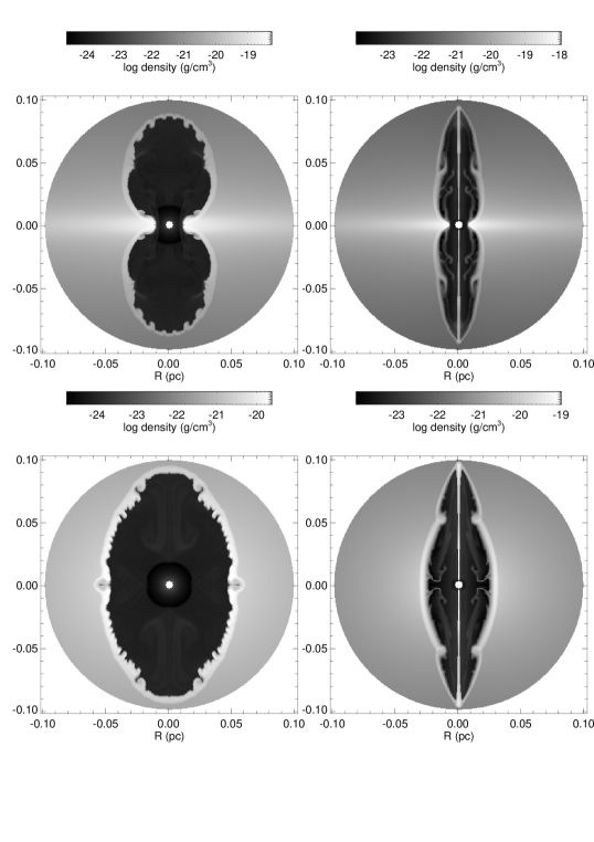
Figure 1: Density distributions of model B at 2500 yr (top-left), model E at 3500 yr (bottom-left), model Bm at 1500 yr (top-right), and model Em at 2000 yr (bottom-right).

3 Morpho-kinematical modeling with SHAPE

In this study, the hydrodynamical simulations serve two purposes. First, we use them as observable objects, of which we know their structure, dynamics and kinematics. For a given time in the evolution, we analyze and visualize the projected images and position velocity (P-V) diagrams as if they where true observations. These images and P-V diagrams are generated with Shape after the data from the simulations have been imported in a suitable format (see below).

The second purpose of using hydrodynamical simulations is to validate the functionality of Shape itself. For this purpose we reproduce the velocity field of the simulation and its structure in detail using the structure and velocity modeling tools of Shape . We then check whether the images and P-V diagrams are consistent with those of the simulation.

We consider only the dense expanding shell that has been swept up by the fast stellar wind. It is this shell, that is expected to be visible as the bright main shell in a planetary nebula. We assume that the nebula is fully ionized and that the emission measure, proportional to the square of the density, provides the relative brightness.

In order to extract the region of the expanding shell we have selected cells from the hydrodynamic simulation according to their radial velocity and density contrast with neighboring cells. The selection is based on the fact that the shell is faster than the external medium (AGB-wind), but slower and denser than the active fast stellar wind.

In Shape, each cell corresponds to a particle with properties of position, velocity and brightness. In order to convert the axi-symmetric two-dimensional hydro-data into a 3-D spatial particle structure, 18 particle copies for each extracted cell have been distributed randomly along the corresponding circle around the cylindrical symmetry axis. The velocity components of the particles have been adjusted according to the rotated position. To visualize, analyze and further process the hydrodynamic simulations we import the simulated particle data into Shape (Version $2.7$).

Since Version 1.0, Shape has an integrated tool for the creation of 3-D structures and their velocity field. The simulated planetary nebula will be used to validate our modeling software, its method and accuracy. The hydrodynamic simulations that we are processing have been performed in spherical coordinates. Because of the cylindrical symmetry, only the radial and the poloidal velocity components are non-cero. Shape has two different modeling modes for the velocity components. One is providing an analytic formula and the other is an editable curve, in which any number of linear segments can be used to describe the magnitude of each velocity component ($v_{r},v_{\theta}$) as a function of the corresponding space coordinate ($r$, $\theta$).

The main shell of the nebula is modeled as a closed surface with cylindrical symmetry using the surface modeling tools in Shape . As an example, Figure 2 we show a visualization of the surface adjusted to run B of the simulations. The surface density of particles is constant within the deviations from the random particle statistics. About $6\times 10^{4}$ particles have been used for each object. In order to model the total emission, the relative particle emissivity is given as a function of position with a similar tool described for the velocity modeling (see above).

For the rendering of the images, the emission is directly integrated along the line of sight. In this work we assume optically thin emission. The resulting raw image is then convolved with a gaussian point-spread-function that models the seeing conditions of an optical observation or the beam of a radiotelescope.

Similarly, a P-V diagram is generated by distributing the emission contained in a simulated spectrograph slit in a position-velocity image (velocity is horizontal and position along the slit is vertical). The raw image is then convolved with an ellipsoidal gaussian that has width and height corresponding to the velocity and spatial resolution of the simulated instrument.

Figure 2: The surface model mesh that has been adjusted to the extracted shell from run B. The dots that are plotted represent only 5 % of the total particles that have been stochastically applied to sample the object.

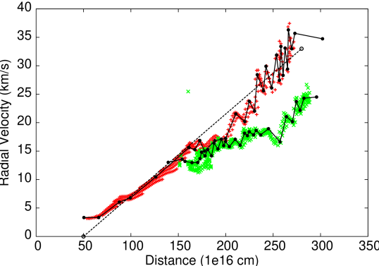
Figure 3: The radial velocity component of the ellipsoidal and bipolar lobed hydrodynamical simulations (E & B)is plotted against the distance from the center. The lines represent the piecewise linear representation of the velocity field in Shape. The dotted line is a simplified approximation with a single linear curve. The simulated data marked by (+) show those of model B and those marked as (x) are from model E.

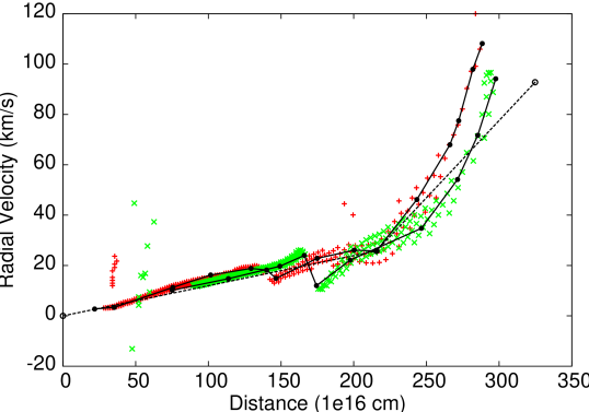
Figure 4: The radial velocity component of the MHD-simulations is plotted against the distance from the center. For a description of the lines, see Figure (3). Here, two linear curve segments have been adopted for the simplified velocity field. The simulated data marked by (+) show those of model Bm and those marked as (x) are from model Em.

Figure 5: The poloidal velocity component of the ellipsoidal and bipolar lobed hydrodynamical simulations is plotted against the angle in degrees from the symmetry axis (equator = $90^{o}$). For a description of the lines and symbols, see Figure (3). Here, two linear curve segments have been adopted for the simplified velocity field.

Figure 6: The poloidal velocity component of the MHD collimated simulations is plotted against the angle in degrees from the symmetry axis (equator = $90^{o}$). For a description of the lines and symbols, see Figure (4). Here, three linear curve segments have been adopted for the simplified velocity field.

4 Results and discussion

In order to search for systematic tell-tale signatures which might reveal information about the physics of their initial formation process, we have investigated the kinematics of typical expanding planetary nebulae based on 4 hydrodynamic simulations (Figure 1).

Figures 3 and 4 show the distribution of the radial velocities ($v_{r}$) of the four simulations as a function of distance from the center. Figures 5 and 6 display the poloidal velocity ($v_{\theta}$) component as a function of the angle from the polar axis of the simulations. For software validation the graphs have been approximated in Shape using piece-wise linear segments as shown by the continuous lines with dots superimposed on the data from the simulations. The resulting P-V diagrams follow those of the simulation to within the scatter of the points from the simulation, validating the our Shape code.

Figures (7) to (10) show the rendered hydrodynamical simulations (columns ”a”), their slit-less spectra or Hubble-like reconstructions (columns ”b”) and the reconstructed models with Shape (columns ”c”). For the slit-less spectra, the simulated spectrograph slit was opened to include the complete object. Note that a slit-less spectrum is equivalent to a 3D reconstruction that makes the assumption of a ”Hubble-type” velocity distribution, projected perpendicular to the line of sight. A small gaussian blur has been applied to simulate observational seeing and reduce the stochastic particle-noise. We discuss the results for each simulation separately.

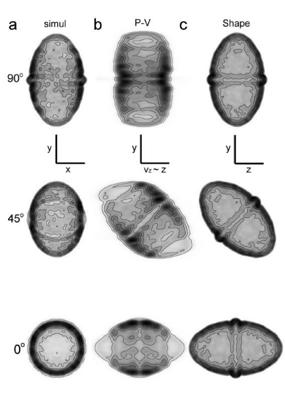
Figure 7: Column ”a”shows the rendered images (emission measure) of the hydrodynamical simulation E at different inclination angles ($0^{o},45^{o},90^{o}$) as seen from the observer’s point of view. Column ”b” contains the corresponding slit-less spectra of the simulation. It represents the view of the object as seen perpendicular to the line of sight in a reconstruction that is based on homologous expansion. This image reveals the deformations expected from such reconstructions. Despite of the cylindrical symmetry of the object, the shape of the ”reconstruction” is quite different to the direct image of the simulation in column ”a”. Column ”c” shows the rendered image of our model as reconstructed with Shape (column ”c”) with corrections to the homologous expansion velocity field as seen from the same direction as column ”b”.

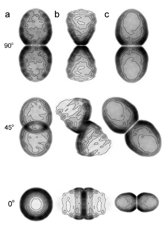
Figure 8: The rendered images of the hydrodynamical simulation B (column ”a”), slit-less spectra or homologous reconstruction (column ”b”) and the rendered image of the reconstructed model with Shape (column ”c”). For further descriptions see Figure (7).

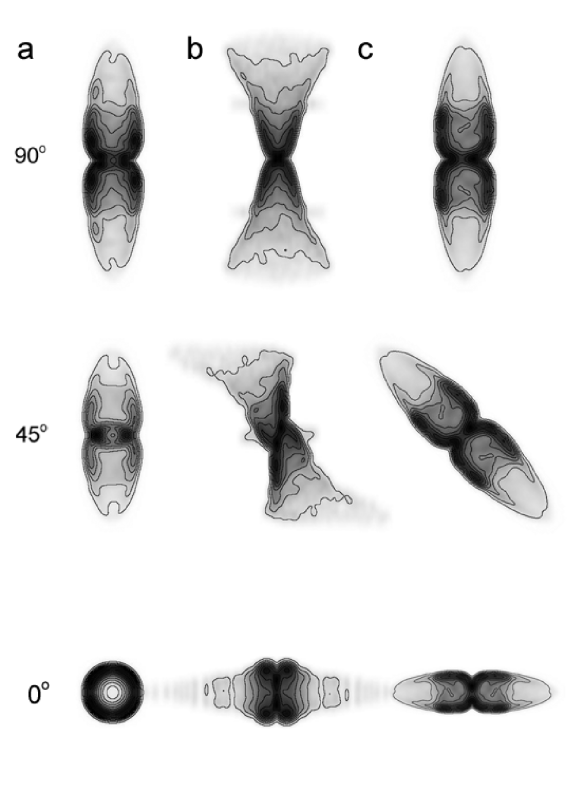
Figure 9: The rendered images of the hydrodynamical simulation Em (column ”a”), slit-less spectra or homologous reconstruction (column ”b”) and the rendered image of the reconstructed model with Shape (column ”c”). For further descriptions see Figure (7).

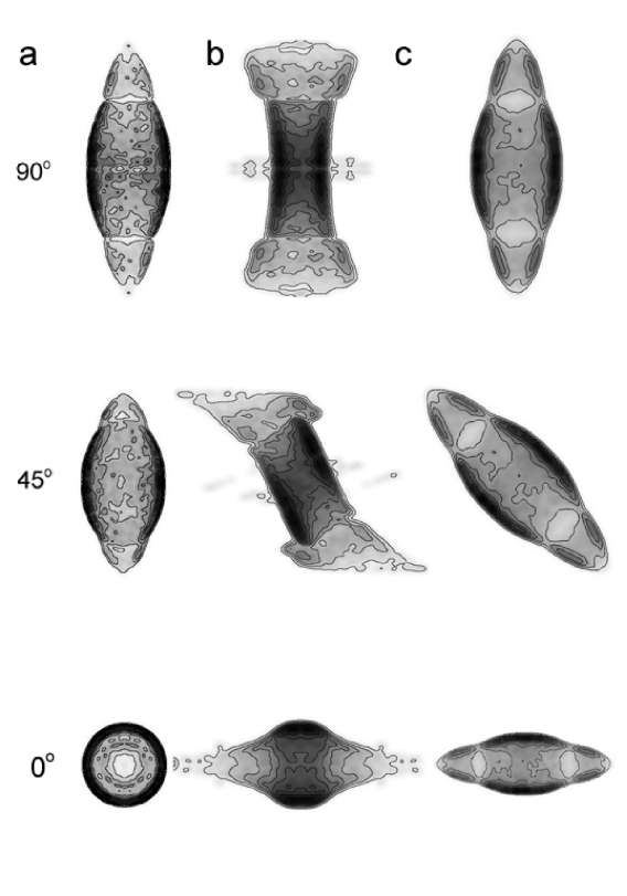
Figure 10: The rendered images of the hydrodynamical simulation Bm (column ”a”), slit-less spectra or homologous reconstruction (column ”b”) and the rendered image of the reconstructed model with Shape (column ”c”). For further descriptions see Figure (7).

4.1 Non-MHD elliptical nebula

Figures (3) and (5) show the statistics of the velocity component distribution in the hydrodynamical simulation of run E which produced an ellipsoidal nebula (Figure 7). The radial velocity component increases approximately linearly with distance (Figure 3). This might suggest that a homologous expansion is a good description of the velocity field. However, the plot of the poloidal velocity component versus position angle reveals that there are deviations of the velocity vector from the radial direction (Figure 5). The deviations increase from the equator to poles until they reach approximately 7 km s^-1 at 20 $\deg$ from the pole. Close to the poles the poloidal velocity decreases again to zero. Where the poloidal component is largest, noticeable deformations will occur along the line of sight in a 3D reconstruction that assumes a homologous expansion law.

The image, the slit-less spectra and the reconstructed models are compared in Figure (7). The shape of the slit-less spectrum at $90^{o}$ (b) is more rectangular than the direct image (a). However, the reconstructed model (c) fits quite well. Although the deviations in (b) are small they are significant at intermediate to high latitudes. For the $0^{o}$ and $90^{o}$ viewing angles, the qualitative difference is small and therefore might not influence significantly the physical interpretation of the object. However, at intermediate viewing angles the P-V diagram is more distorted and becomes point-symmetric. We consider it cautiously acceptable to directly reconstruct this type of objects from their spectral data assuming a homologous expansion law.

Both, the radial and the poloidal velocity show small-scale fluctuations which are associated with local instabilities. In a reconstruction, unresolved fluctuations will result in an increased thickness of the reconstructed surface structure.

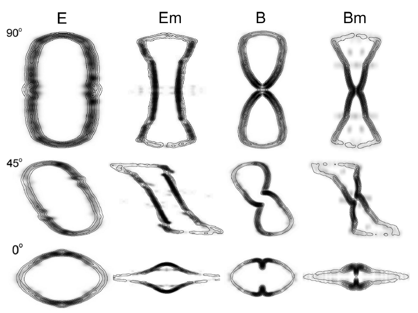
Figure 11: Central slit P-V diagrams from the simulations are represented in grey-scale. The superimposed contours are from the same simulations, but with a simple piece-wise linear velocity distributions applied (dashed lines in Figures (3) to (6).

4.2 Non-MHD bipolar lobes

The radial velocity distribution for the bipolar lobes from the purely hydrodynamic model B is shown in Figure (3) and the distribution of the poloidal velocity is given in Figure (5). As in the ellipsoidal case of run E, we find a nearly linear increase of the radial velocity component with distance. Deviations from linearity are stronger far away and very close to the center. Also, the small-scale fluctuations increase at a certain distance. This distance marks the transition between two different dynamical regions in this bipolar nebula.

The general trend of the poloidal velocity is similar to the one in the ellipsoidal simulation, a linear increase with angle up to a maximum value and then a decrease towards the pole. The vanishing poloidal velocity at the pole and the equator are enforced in these simulations due to the boundary conditions of reflection at the equator and polar axis. However, it is expected that this behavior is very closely sustained in real objects with approximate axi-symmetry.

Column ”b” in Figure (8) shows the slitless spectra of simulation B for 3 different viewing angles. This corresponds to a 3D reconstruction that assumes homologous expansion as viewed along a direction perpendicular to the observer’s line of sight. We note very significant differences to the observer’s view in column ”a”. Especially, the ”Hubble-type reconstructions” at $45^{o}$ and $0^{o}$ inclination angles show strong deviations. As in the case of run E, the intermediate angles introduce a point-symmetry which is now even stronger. Column ”c” of Figure (8) shows the corresponding views of the axi-symmetric reconstructed model using Shape which applies the simple piece-wise linear velocity law (see below).

In order to not only reproduce the images, but also the P-V diagrams with a model that improves the homologous expansion law with only a few additional parameters, we propose a simple piece-wise linear approximation to the velocity components as a function of position.

For runs E and B, a two-parameter curve of two linear segments that start at zero at the pole and equator and meet at a point ($\theta$, v_θ) are sufficient. The point ($\theta$, v_θ) is a free parameter of the model. In addition, a linear relation of the radial velocity with distance could be used. The result of such a fit is shown in the P-V diagrams of Figure (11, column E & B). The grey-scale P-V diagrams are from the hydrodynamical simulations with its original velocity information. The contours are from the same structural data, but with the new simple piece-wise linear velocity field. As an example, the corresponding velocity components of run B are plotted as dotted lines in Figures (3) & (5).

We find that the agreement of this simple piece-wise linear velocity field with the simulation is very satisfactory. At any viewing angle deviations in the P-V diagram are only significant at the small scales of instabilities. Hence, for an elliptical or bipolar hydrodynamical nebula a very significant improvement in its morpho-kinematical modeling may be achieved by including only one and two linear segments in the distribution of the radial and poloidal velocity components, respectively. This procedure retains the axi-symmetric structure of the object and, simultaneously, provides a good fit to the point-symmetric P-V diagrams.

4.3 MHD collimated nebulae

We now perform a similar analysis to the MHD-simulations. Figure (4) shows the distribution of the radial velocity components of simulations Bm and Em as a function of distance from the center. The poloidal velocity component is plotted in Figure (6). Both simulations show similar velocity fields, but with different positions and amplitudes of the dynamical regions. The radial velocity component has a nearly linear increase up to about half of the extent of the nebula. Then an abrupt change is noticeable with a small drop in the velocity and further out a significant gradual increase in the slope of the velocity graph.

The poloidal velocity component is slowly growing from the equator towards the pole and shows an accelerated increase from mid-latitudes on. It reaches a maximum near the tip of the outflow, after which it declines rapidly (as expected from the symmetry of the flow, see above). There are no strong small-scale variations in either velocity component as opposed to those found in the purely hydrodynamic simulations.

Figures (9) and (10) compare the projected images rendered from the MHD-simulations (column “a”) with the “3D Hubble-type reconstructions”, i.e., the slit-less spectra (column “b”), and the reconstructed model using Shape (column “c”). The distortions observed in columns ”b” are even stronger than in the non-MHD simulations. Instead of being closed bipolar lobes, they appear to be open. In all cases of intermediate inclination angles, the axi-symmetry of the simulation is lost and replaced by point-symmetry. A physical interpretation of such artificial symmetry features, in 3D reconstructions that assume homologous expansion, may lead to seriously erroneous results.

In order to capture the main features of the velocity field in this type of objects in morpho-kinematical modeling, we propose to use at least two linear segments for the radial component and three segments for the poloidal velocity component. Such approximations for model Bm have been plotted in Figures (4) and (6) as dotted lines. See Figure (11) to compare the P-V diagrams from the simplified Shape model with those of the simulation. The deviations from the simulation are very small, hence, also for the MHD cases a considerable improvement of the velocity field can be obtained by the simple piece-wise linear velocity field proposed here.

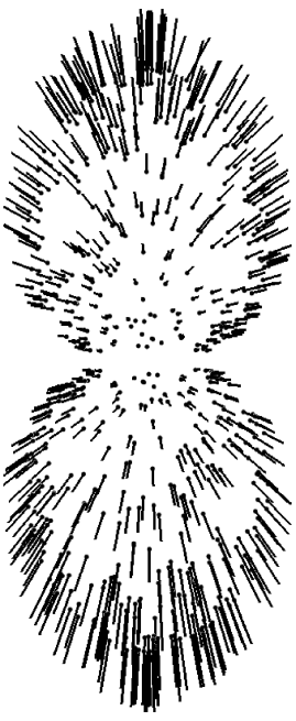
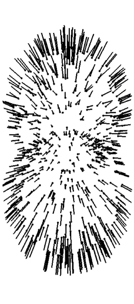
Figure 12: Proper motion vectors are shown for model B at 90 and 45 degrees viewing angle on the left and right, respectively. The top half has the velocity field as obtained from the simulation, while the bottom has a homologous expansion law.

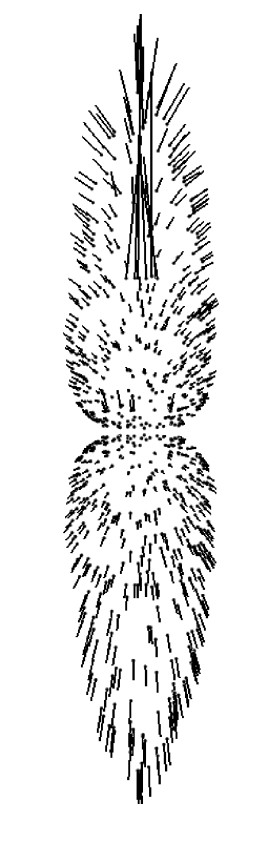
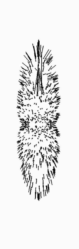
Figure 13: Proper motion vectors are shown for model Bm at 90 and 45 degrees viewing angle on the left and right, respectively. The top half has the velocity field as obtained from the simulation, while the bottom has a homologous expansion law. The top half includes part of the central collimated outflow with very large velocity vectors.

5 Proper motion patterns

Additional kinematic information from an expanding object can be obtained from internal proper motion measurements. Such measurements have been obtained for a few nearby planetary nebulae (e.g. NGC6302: Meaburn et al. 2008; NGC7009: Rodríguez & Gómez 2007). Measurements of Doppler-shift and proper motion of a large number of features in a nebula (e.g. Li, Harrington & Borkowski 2002) might reveal whether an object is hydrodynamically active or expanding homologously due to ballistic motion. In Figures (12) and (13) we compare the proper motion vectors of our simulations B and Bm with the corresponding homologous motion patterns for two different viewing angles. The top halves of the images represent the velocity pattern from the hydrodynamical simulations, while in the bottom halves we replaced the original velocity field by a homologous velocity field. Clearly, such measurements might reveal a lot of information about the dynamical state of a planetary nebula. When the expansion is homologous, the proper motion pattern reflects this in purely radial vectors with magnitudes that increase linearly with distance. This pattern is basically independent of the structure and orientation of the object.

However, in a dynamically active nebula or in a nebula with several kinematic sub-systems, the motion pattern will depend on the orientation and structure. Some of the proper motion vectors in Figures (12) and (13) almost reverse direction in the inclined objects (right side). Such a behavior is found in BD+30^o3639. As seen from the proper motion pattern in Li, Harrington & Borkowski (2002), BD+30^o3639 is likely to still be a dynamically active nebula. The spectral and proper motion data from Meaburn et al. (2008) indicate that NGC 6302 is expanding radially and, hence, presumably ballistically.

In general, because of the evolution of the fast stellar wind, it is expected that young planetary nebulae will be more likely to be active than older nebulae. It is therefore surprising that very young non-spherical nebulae, like, for instance, Minkowski’s footprint (M1-92, Alcolea, Neri & Bujarrabal 2007) show Doppler-shift patterns that are consistent with axi-symmetric homologous expansion. It is important to systematically survey the kinematic properties of planetary nebulae for evidence of deviations from homologous expansion. This will reveal information about the evolution of the fast stellar wind and the evolution of central stars in general. Hopefully, the analysis of large kinematical catalogs like those of Hajian et al. (2007) and López et al. (2006) might be helpful in studying the transition phase between hydrodynamically active and ballistic expansion.

6 Conclusions

Based on axi-symmetric hydrodynamical simulations and 3D reconstructions with the software package Shape, we have investigated the kinematic signatures of deviations from “Hubble-type” outflows in some typical shapes of planetary nebulae. The deviations are systematic and their description as given in this paper may help to improve morpho-kinematic and dynamic models of planetary nebulae. Excluding the small-scale variations from local instabilities, we find that the radial velocity as a function of distance can be well described by a linear increase for the cases of purely hydrodynamical ellipsoidal and bipolar-lobed nebulae. The poloidal component is, however, not negligable. Its parameterized approximation requires two linear segments, one increasing and the other decreasing with zero velocity at the pole and equator. We also find that the magneto-hydrodynamically generated cases require two linear segments for the radial velocity component and three segments for the poloidal component. These simple extensions to a homologous expansion law capture the global velocity structure of hydrodynamically active axi-symmetric nebulae except for small-scale variations.

We find that, in most situations considered in our simulations, the deviations from a homologous flow, both in magnitude and direction of the velocity vector, are significant and observable. The only case where only small deviations were found was the case of an ellipsoidal nebula.

If significant deviations from a homologous expansion model can be inferred, then it is very likely that it is still dynamically active in the sense that the fast wind is still significant or the inner region of the nebula is still over-pressurized with respect to the exterior. In a future paper we will explore more precisely how the transition from the hydrodynamically to the ballistic regimes occurs.

It is the relative size of the poloidal velocity component that strongly influences the shape of the position velocity diagrams that are obtained, not so much the variation of the radial component with distance from the center. The deviations increase with the degree of collimation of the nebula. They are stronger at intermediate latitudes. There is a slow increase in deviations as we move from the equator to the poles, usually with a sudden increase at mid-latitudes.

A good description of the velocity field in the MHD-simulations requires one more linear segment than that of the non-MHD simulations. This would imply that this difference might provide observational evidence for the presence or absence of dynamical active magnetic fields in the formation process of planetary nebulae. However, this aspect might require more detailed and specific studies.

Summing up, detailed morpho-kinematic observations and modeling of planetary nebulae can reveal whether a nebula is still in a hydrodynamically active stage or whether it has reached ballistic expansion.

References

- (1) Akashi, M., Soker, N., 2008, arXiv:0805.2332v1 [astro-ph]
- (2) Alcolea, J.; Neri, R.; Bujarrabal, V., 2007, A&A, 468. L41-L44
- (3) Bjorkman, J. E. & Cassinelli, J. P. 1993, ApJ, 409, 429
- (4) Chevalier, R. A. & Luo, D. 1994, ApJ, 421, 225
- (5) Clarke, D. A. 1996, ApJ, 457, 291
- (6) Dennis, T. J., Cunningham, A. J., Frank, A., Balick, B., Blackman, E. G. , Mitran, S., 2008, ApJ, 679, 1327-1337
- (7) Dobrinčić, M. and Villaver, E. and Guerrero, M. A. and Manchado, A., 2008, AJ, 135, 2199-2211
- (8) Ercolano, B., Barlow, M. J., Storey, P. J., 2005, MNRAS, 362, 1038-1046
- (9) García-Segura, G., Langer, N., Różyczka, M., & Franco, J. 1999, ApJ, 517, 767
- (10) Hajian, A. R., and Movit, S. M., Trofimov, D., Balick, B., Terzian, Y., Knuth, K. H., Granquist-Fraser, D., Huyser, K. A., Jalobeanu, A., McIntosh, D., Jaskot, A. E., Palen, S., Panagia, N., 2007, ApJS, 169, 289-327
- (11) Ignace, R., Cassinelli, J. P. & Bjorkman, J. E. 1996, ApJ, 459, 671
- (12) Li, J., Harrington, J. P., Borkowski, K. J., 2002, AJ, 123, 2676-2688
- (13) López, J. A., Richer, M., Riesgo, H., Steffen, W., Meaburn, J., Garc a-Segura, G., Escalante, K., 2006, XI IAU Regional Latin American Meeting of Astronomy (Eds. L. Infante & M. Rubio), RMxAC, 26, 161
- (14) Meaburn, J., López, J.A., Steffen, W., Graham, M.F., Holloway, A.J., 2005, , AJ, 130, 2303-2311
- (15) Meaburn, J., LLoyd, M., Vaytet, N.M.H., López, J.A., 2008, MNRAS, 385, 269-273
- (16) Morisset, C., Stasinska, G., 2008, RMxAA, 44, 171-180
- (17) Morisset, C., 2006, IAU proceedings on ”Planetary Nebulae in our Galaxy and Beyond”, 2: 467-468 Cambridge University Press
- (18) O’Connor, J. A., Redman, M. P., Holloway, A. J., Bryce, M., López, J. A., Meaburn, J., 2000, ApJ, 531, 336-344
- (19) Raymond, J. C. & Smith, B. W. 1977, ApJS, 35, 419
- (20) Rodríguez, L.F., Gómez, Y., 2007, RMxAA, 453, 173-177
- (21) Różyczka, M. & Franco, J. 1996, ApJL, 469, L127
- (22) Sabbadin, F. and Turatto, M. and Ragazzoni, R. and Cappellaro, E. and Benetti, S., 2006, A&A, 451, 937-949
- (23) Santander-García, M. Corradi, R. L. M. Balick, B. Mampaso, A., 2004, A&A, 426, 185-194
- (24) Steffen, W., López, J.A., 2004, ApJ, 612, 319-331
- (25) Steffen, W., López, J.A., 2006, RMxAA, 42, 99-105
- (26) Stone, J. M. & Norman, M. L. 1992, ApJS, 80, 753
- (27) Wilson, O., 1950, ApJ, 111, 279