September 2008 UMDEPP-08-018

SUNY-O/667

We explain how the redefinitions of supermultiplet component fields, comprising what we call “frame shifts”, can be used in conjuction with the graphical technology of multiplet Adkinras to render manifest the reducibility of off-shell representations of supersymmetry. This technology speaks to possibility of organizing multiplet constraints in a way which complements and extends the possibilities afforded by superspace methods.

   
PACS: 04.65.+e

Four years ago, in  [?], graphical devices for representing supermultiplets were introduced. We have used these tools frequently since that time, as we find these distinctly useful for organizing various open questions about supersymmetry. Moreover, these graphs illuminate intriguing emergent mathematical features of supersymmetry not manifest in the context of more traditional methods, such as superspace. Accordingly, we have been incrementally adding mathematical sophistication to this technology  [?,?,?,?]. For reasons explained in  [?], we refer to our graphical representations of supermultiplets as Adinkras. In the case of one-dimensional supersymmetry we have developed a means, reminiscent of Feynman rules, which allows unambiguous translation of supersymmetry transformations from these graphs. In four-dimensions the technology is less-developed, and the graphs serve more as helpful visual aids. However, there is an especially useful feature exhibited by four-dimensional Adinkras concerning how the graphical structures may be manipulated to expose and render obvious when and how the multiplet admits projection to submultiplets. The primary goal of this letter is to explain this.

We should point out that the analysis of the reduction of $N=1$ supermultiplets described in this letter is an old and well known story, described in many places, e.g.  [?,?]. But the methodology which we bring to bear on this problem is new and interesting. We believe that practitioners of supersymmetry will appreciate the fresh look that this perspective brings to this matter, especially as regards its potential for resolving related issues in higher-$N$ supersymmetry, where superspace methods become increasingly cumbersome.

The basic idea behind Adinkras is a deceptively simple one: to construct graphs by representing fields as vertices which are interconnected pairwise by edges when the corresponding fields are related by supersymmetry transformations. No-doubt practitioners have done this sort of thing ever since supersymmetry was first conceived in the early 1970s. However, it has become increasingly evident that such diagrams encode a wealth of information which may be extracted beneficially to complement or even replace some traditional methods for organizing and classifying supermultiplets and supersymmetric actions. As a notable example, the one-dimensional Adinkras obtained by dimensional reduction of supermultiplets in any number of dimensions admit topological classification in terms of doubly-even linear binary codes  [?].

One of our prime motivations has been to better understand the nexus of ways in which higher-$N$ theories may be realized off-shell. One preliminary result obtained using our methods was the discovery of a way to couple what we call quadruplet matter to $N=2$ hypermultiplets, using a finite number of off-shell degrees of freedom. This was explained in  [?]. That work exposed deeper questions, which we hope to resolve, concerning the possibility of removing the quadruplet matter to expose an interesting new off-shell realization of a pure hypermultiplet. Our scrutiny of this question impelled us investigate structures in  [?] using the simpler setting of $N=1$ supersymmetry; the results of this letter derived from that investigation. All of this has a deeper motivation related to our desire to develop either an off-shell realization of $N=4$ Super Yang-Mills theory involving a finite number of component fields, or to prove that such constructions are precluded within the ordinary framework of supersymmetric quantum field theory. The latter is a commonly-held belief which we have not found demonstrably substantiated in the literature.

As explained above, an Adinkra consists of a set of vertices, one for each component field in a given supermultiplet. These vertices are connected pairwise by edges when the corresponding component fields are connected by a supersymmetry transformation. We color boson vertices white, and we color fermion vertices black. In four-dimensions, multiplet component fields comprise irreducible representations of $\mathfrak{spin}(3,1)$; we use a single vertex for each such field and decorate this with a numeral to indicate the number of off-shell degrees of freedom described by that field. For example, a complex scalar boson would be represented by a white vertex decorated with the numeral 2. Next, we organize the vertices vertically in a manner which faithfully respects the engineering dimension of the fields, with lower-dimension fields at the bottom of the diagram and higher-dimension fields placed at successively higher “levels”.

As a simple example, the Chiral multiplet consists of a complex scalar $\phi$, a right-handed Weyl spinor $\psi_{R}$, and a higher-weight complex scalar $F$. This multiplet has the following supersymmetry transformation rules,

$$\delta_{Q}\,\phi = i\,\bar{\epsilon}_{L}\,\psi_{R}$$

$$\delta_{Q}\,\psi_{R} = \hbox{\ooalign{$\displaystyle\partial$\cr$/$}}\,\phi\,\epsilon_{L}+F\,\epsilon_{R}$$ (3)

$$\delta_{Q}\,F = i\,\bar{\epsilon}_{R}\,\hbox{\ooalign{$\displaystyle\partial$\cr$/$}}\,\psi_{R}\,,$$ (6)

where $\epsilon_{L}$ is a left-handed Weyl spinor supersymmetry parameter and $\epsilon_{R}$ is its Majorana conjugate. We represent this multiplet by the following Adinkra,

$$\vbox{\hbox{\hss\includegraphics[width=50.58878pt]{A_Chi.pdf}\hss}}\,.$$ (7)

Under (6) the complex scalar $\phi$ transforms into the spinor $\psi_{R}$, and the spinor $\psi_{R}$ transforms into the derivative of the scalar; for these reasons the $\phi$ vertex and the $\psi_{R}$ vertex are connected by a black edge in the diagram (7). Similarly, the spinor $\psi_{R}$ transforms into the complex scalar $F$ while this field transforms into the derivative of the spinor; for these reasons the $\psi_{R}$ node is connected by a black edge to the $F$ node.

In the Chiral Adinkra (7) each edge represents two terms in the transformation rules (6): one “upward-directed” under which a lower-weight field transforms into a higher-weight field, and one “downward directed” in which a higher-weight field transforms into the derivative of the lower-weight field. Conventionally, the black-coloration of an edge denotes this bidirectional quality. As it turns out, it is possible to structure some transformation rules so that a given upward-directed term does not have a downward-directed counterpart; we give explicit examples of this below. In such a circumstance, we denote an upward-directed term which does not have a downward-directed counterpart using a grey, rather than a black, edge.

Consider next a Real Scalar multiplet $V$ as described by the following component supersymmetry transformation rules,

$$\delta_{Q}\,b = {\textstyle\frac{1}{2}}\,i\,\bar{\epsilon}\,\chi$$

$$\delta_{Q}\,\chi = \hbox{\ooalign{$\displaystyle\partial$\cr$/$}}\,b\,\epsilon+{\textstyle\frac{1}{2}}\,i\,A_{a}\,\gamma^{a}\gamma_{5}\,\epsilon+{\textstyle\frac{1}{2}}\,f\,\epsilon-{\textstyle\frac{1}{2}}\,i\,g\,\gamma_{5}\,\epsilon$$ (10)

$$\delta_{Q}\,f = {\textstyle\frac{1}{2}}\,i\,\bar{\epsilon}\,\hbox{\ooalign{$\displaystyle\partial$\cr$/$}}\chi+{\textstyle\frac{1}{2}}\,i\,\bar{\epsilon}\,\lambda$$ (13)

$$\delta_{Q}\,g = {\textstyle\frac{1}{2}}\,\bar{\epsilon}\,\gamma_{5}\,\hbox{\ooalign{$\displaystyle\partial$\cr$/$}}\chi+{\textstyle\frac{1}{2}}\,\bar{\epsilon}\,\gamma_{5}\lambda$$ (16)

$$\delta_{Q}\,A_{a} = {\textstyle\frac{1}{2}}\,\bar{\epsilon}\,\gamma_{5}\,\hbox{\ooalign{$\displaystyle\partial$\cr$/$}}\gamma_{a}\,\chi-{\textstyle\frac{1}{2}}\,\bar{\epsilon}\,\gamma_{a}\gamma_{5}\,\lambda$$ (19)

$$\delta_{Q}\lambda = {\textstyle\frac{1}{2}}\,\hbox{\ooalign{$\displaystyle\partial$\cr$/$}}f\,\epsilon-{\textstyle\frac{1}{2}}\,i\,\hbox{\ooalign{$\displaystyle\partial$\cr$/$}}g\,\gamma_{5}\,\epsilon+{\textstyle\frac{1}{2}}\,i\,\gamma^{a}\hbox{\ooalign{$\displaystyle\partial$\cr$/$}}\,A_{a}\,\gamma_{5}\,\epsilon+D\,\epsilon$$ (26)

$$\delta_{Q}\,D = {\textstyle\frac{1}{2}}\,i\,\bar{\epsilon}\,\hbox{\ooalign{$\displaystyle\partial$\cr$/$}}\,\lambda\,.$$ (29)

where the scalar component field $b$ is assigned even parity. The parity of all other components then follows from the requirement that a parity flip commute with supersymmetry; for example $\chi$ and $\lambda$ each have even parity, $g$ is a pseudoscalar, and $A_{a}$ is an axial vector.

Consider also a Real Pseudoscalar multiplet $\tilde{V}$ as described by the following component supersymmetry transformation rules,

$$\delta_{Q}\,\tilde{b} = {\textstyle\frac{1}{2}}\,\bar{\epsilon}\,\gamma_{5}\,\tilde{\chi}$$

$$\delta_{Q}\,\tilde{\chi} = i\,\gamma_{5}\hbox{\ooalign{$\displaystyle\partial$\cr$/$}}\,\tilde{b}\,\epsilon-{\textstyle\frac{1}{2}}\,V_{a}\,\gamma^{a}\,\epsilon+{\textstyle\frac{1}{2}}\,\tilde{f}\,\epsilon-{\textstyle\frac{1}{2}}\,i\,\tilde{g}\,\gamma_{5}\,\epsilon$$ (32)

$$\delta_{Q}\,\tilde{f} = {\textstyle\frac{1}{2}}\,i\,\bar{\epsilon}\,\hbox{\ooalign{$\displaystyle\partial$\cr$/$}}\tilde{\chi}+{\textstyle\frac{1}{2}}\,i\,\bar{\epsilon}\,\tilde{\lambda}$$ (35)

$$\delta_{Q}\,\tilde{g} = {\textstyle\frac{1}{2}}\,\bar{\epsilon}\,\gamma_{5}\,\hbox{\ooalign{$\displaystyle\partial$\cr$/$}}\tilde{\chi}+{\textstyle\frac{1}{2}}\,\bar{\epsilon}\,\gamma_{5}\tilde{\lambda}$$ (38)

$$\delta_{Q}\,V_{a} = {\textstyle\frac{1}{2}}\,i\,\bar{\epsilon}\,\hbox{\ooalign{$\displaystyle\partial$\cr$/$}}\gamma_{a}\,\tilde{\chi}+{\textstyle\frac{1}{2}}\,i\,\bar{\epsilon}\,\gamma_{a}\,\tilde{\lambda}$$ (41)

$$\delta_{Q}\,\tilde{\lambda} = {\textstyle\frac{1}{2}}\,\hbox{\ooalign{$\displaystyle\partial$\cr$/$}}\tilde{f}\,\epsilon+{\textstyle\frac{1}{2}}\,i\,\gamma_{5}\hbox{\ooalign{$\displaystyle\partial$\cr$/$}}\tilde{g}\,\epsilon-{\textstyle\frac{1}{2}}\,\gamma^{a}\hbox{\ooalign{$\displaystyle\partial$\cr$/$}}\,V_{a}\,\epsilon-i\,\tilde{D}\,\gamma_{5}\,\epsilon$$ (48)

$$\delta_{Q}\,\tilde{D} = {\textstyle\frac{1}{2}}\,\bar{\epsilon}\,\gamma_{5}\hbox{\ooalign{$\displaystyle\partial$\cr$/$}}\,\tilde{\lambda}\,.$$ (51)

The distinction between this multiplet and (29) pertains to the parity of the lowest component scalar fields; in this case the component $\tilde{b}$ is assigned odd parity. It follows that $\tilde{\chi}$ and $\tilde{\lambda}$ each have even parity, the fields $\tilde{g}$ and $\tilde{D}$ are each pseudoscalars, while the vector $V_{a}$ has even parity.

Taken together, the transformation rules (29) and (51) are represented diagrammatically as in Figure 1,

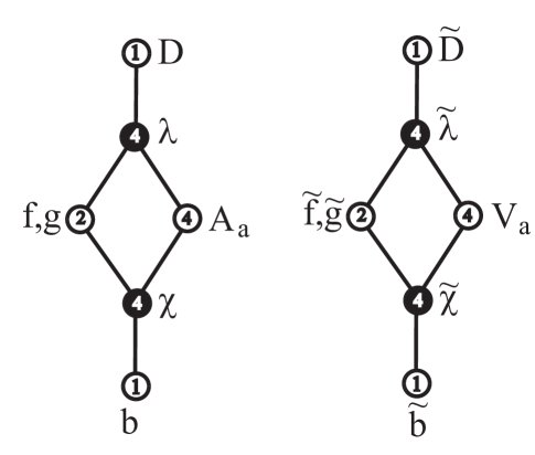
Figure 1: The real and imaginary parts of a Complex Scalar multiplet correspond to a Real Scalar multiplet (29) and a Real Pseudoscalar multiplet (51), respectively. These are represented above using a disconnected Adinkra.

where a single combined vertex represents $f$ and $g$ together, and another combined vertex represents $\tilde{f}$ and $\tilde{g}$. The fact that Figure 1 has two disconnected parts reflects the fact that the fields in the multiplet $V$ do not transform into the fields in $\tilde{V}$, and vice-versa. This pair admits an obvious complex structure allowing us to define ${\mathbb{V}}:=V+i\,\tilde{V}$. The reducibility of the combined mutliplet is manifest using the diagram in Figure 1, since one can constrain all of the fields in either disconnected piece to vanish, an operation which is consistent with supersymmetry owing to the disconnected feature of the diagram.

The transformation rules (29) and (51) describe together the component version of the transformations generated by the supercharge $Q$ acting on an unconstrained $N=1$ superfield corresponding to ${\mathbb{V}}$. From the point of view of superspace, the restriction to the submultiplet described by the connected diagram on the left-side of Figure 1, effected by constraining the connected diagram on the right-side to vanish, is equivalent to the superfield constraint ${\mathbb{V}}={\mathbb{V}}^{\dagger}$, where the complex structure described above has been implied. Similarly, the restriction to the other connected sub-multiplet is equivalent to the superspace constraint ${\mathbb{V}}=-{\mathbb{V}}^{\dagger}$.

Since we have assigned positive parity to $V$ and negative parity to $\tilde{V}$, so that $b$ and $\tilde{b}$ describe a respective scalar and a pseudoscalar, it follows that we can sensibly reorganize the component fields using the following definitions,

$$B := b-i\,\tilde{b}$$

$$\xi_{L} := {\textstyle\frac{1}{2}}\,(\,\chi_{L}+\tilde{\chi}_{L}\,)$$

$$\rho_{R} := {\textstyle\frac{1}{2}}\,(\,\chi_{R}-\tilde{\chi}_{R}\,)$$

$$P_{a} := -{\textstyle\frac{1}{4}}\,(\,V_{a}-i\,A_{a}\,)+{\textstyle\frac{1}{2}}\,\partial_{a}\,(\,b-i\,\tilde{b}\,)$$

$$H := -{\textstyle\frac{1}{2}}\,(\,\tilde{f}-i\,\tilde{g}\,)$$

$$\beta_{L} := {\textstyle\frac{1}{4}}\,(\,\lambda_{L}-\hbox{\ooalign{$\displaystyle\partial$\cr$/$}}\,\chi_{R}\,)+{\textstyle\frac{1}{4}}\,(\,\tilde{\lambda}-\hbox{\ooalign{$\displaystyle\partial$\cr$/$}}\,\tilde{\chi}_{R}\,)$$ (56)

$$\phi := {\textstyle\frac{1}{2}}\,(\,f+\tilde{f}\,)+{\textstyle\frac{1}{2}}\,i\,(\,g+\tilde{g}\,)$$

$$\psi_{R} := {\textstyle\frac{1}{2}}\,(\,\lambda_{R}+\hbox{\ooalign{$\displaystyle\partial$\cr$/$}}\,\chi_{L}\,)+{\textstyle\frac{1}{2}}\,(\,\tilde{\lambda}_{R}+\hbox{\ooalign{$\displaystyle\partial$\cr$/$}}\,\tilde{\chi}_{L}\,)$$ (61)

$$F := {\textstyle\frac{1}{2}}\,(\,D+\partial^{a}V_{a}-\Box\,b\,)-{\textstyle\frac{1}{2}}\,i\,(\,\tilde{D}+\partial^{a}A_{a}-\Box\,\tilde{b}\,)\,.$$ (62)

By replacing the fields $(\,b\,,\,\chi\,,\,f\,,\,g\,,\,A_{a}\,,\,\lambda\,,\,D\,)$ and $(\,\tilde{b}\,,\,\tilde{\chi}\,,\,\tilde{f}\,,\,\tilde{g}\,,\,V_{a}\,,\,\tilde{\lambda}\,,\,\tilde{D}\,)$ with the equivalent set of fields defined by $(\,B\,,\,\rho\,,\,H\,,\,\xi\,,\,P_{a}\,,\,\beta\,,\,\phi\,,\,\psi\,,\,F\,)$ we have “changed frames” in the space defined by these fields; in either guise the same 16+16 local off-shell degrees of freedom are expressed, albeit in terms of different linear combinations. When re-expressed in terms of the redefined fields, the transformation rules (29) become

$$\delta_{Q}\,B = i\,\bar{\epsilon}_{L}\,\rho_{R}+i\,\bar{\epsilon}_{R}\,\xi_{L}$$

$$\delta_{Q}\,\xi_{L} = P_{a}\,\gamma^{a}\,\epsilon_{R}+{\textstyle\frac{1}{2}}\,\phi\,\epsilon_{L}$$

$$\delta_{Q}\,\rho_{R} = \hbox{\ooalign{$\displaystyle\partial$\cr$/$}}\,B\,\epsilon_{L}-P_{a}\,\gamma^{a}\,\epsilon_{L}+H\,\epsilon_{R}$$ (65)

$$\delta_{Q}\,P_{a} = -{\textstyle\frac{1}{2}}\,i\,\bar{\epsilon}_{R}\,\hbox{\ooalign{$\displaystyle\partial$\cr$/$}}\gamma_{a}\,\xi_{L}+{\textstyle\frac{1}{2}}\,i\,\bar{\epsilon}_{L}\,\gamma_{a}\,\beta_{L}-{\textstyle\frac{1}{4}}\,i\,\bar{\epsilon}\,\gamma_{a}\,\psi$$ (68)

$$\delta_{Q}\,H = i\,\bar{\epsilon}_{R}\,\hbox{\ooalign{$\displaystyle\partial$\cr$/$}}\,\rho_{R}+i\,\bar{\epsilon}_{R}\,\beta_{L}$$ (71)

$$\delta_{Q}\,\beta_{L} = -\gamma^{a}\hbox{\ooalign{$\displaystyle\partial$\cr$/$}}\,P_{a}\,\epsilon_{L}+{\textstyle\frac{1}{2}}\,F\,\epsilon_{L}$$ (74)

$$\delta_{Q}\,\phi = i\,\bar{\epsilon}_{L}\,\psi_{R}$$

$$\delta_{Q}\,\psi_{R} = \hbox{\ooalign{$\displaystyle\partial$\cr$/$}}\,\phi\,\epsilon_{L}+F\,\epsilon_{R}$$ (77)

$$\delta_{Q}\,F = i\,\bar{\epsilon}_{R}\,\hbox{\ooalign{$\displaystyle\partial$\cr$/$}}\,\psi_{R}\,.$$ (80)

Note that the transformation rules (29) and (80) are completely equivalent; these represent the same multiplet in two different “frames”. The second guise for the transformation rules, (80), is represented diagrammatically as in Figure 2.

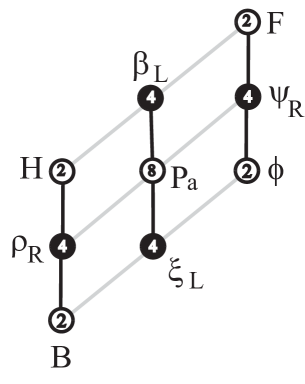
Figure 2: The Complex Scalar multiplet may be expressed in a special “frame” in which the Adinkra has the manifest structure of a Chiral multiplet linked to a Variant Vector multiplet in-turn linked to a higher-weight Chiral multiplet, where the linking are codified by “one-way” grey edges, as explained in the text.

In Figure 2, the grey edges describe upward-directed terms in (80) which do not have downward-directed counterparts. For example the grey edge connecting the $B$ vertex to the $\xi_{L}$ vertex represents the term $i\,\bar{\epsilon}_{R}\,\xi_{L}$ appearing in $\delta_{Q}\,B$. The fact that this edge is grey, rather than black, indicates the interesting fact that there is no term proportional to $B$ which appears in $\delta_{Q}\,\xi_{L}$; thus, the upward-directed term does not have a downward-directed counterpart. Similar comments apply to all six of the grey edges in 2.

The ostensibly distinct Adinkras in Figures 1 and 2 describe precisely the same multiplet expressed in two different frames; these frames are related by the field redefinition (62). In the second frame, the graph shown in Figure 2 exhibits an interesting structure: The fields $B$, $\rho_{R}$, and $H$ transform into each other via two bi-directional term pairs represented by the two black edges which interconnect the corresponding vertices, but none of the remaining fields transform into $B$, $\rho_{R}$, or $H$. Instead, the three upward-directed terms in (80) represented by the three grey edges connecting $B$ with $\xi_{L}$, $\rho_{R}$ with $P_{a}$, and $H$ with $\beta_{L}$, have no downward-directed counterparts. Thus, the subset of fields $(\,B\,,\,\rho_{R}\,,\,H\,)$ connects to $(\,\xi_{L}\,,\,P_{a}\,,\,\beta_{L}\,)$ only via grey edges. In a similar way, the subset $(\,\xi_{L}\,,\,P_{a}\,,\,\beta_{L}\,)$ connects to $(\,\phi\,,\,\psi_{R}\,,\,F\,)$ only by grey edges.

The subset of fields $(\,B\,,\,\rho_{R}\,,\,H\,)$ have transformation rules identical to that of a Chiral multiplet augmented by the addition of three “one-way” terms corresponding to grey edges. As a suggestive mnemonic, we refer to this situation by calling $(\,B\,,\,\rho_{R}\,,\,H\,)$ a Chiral multiplet “flying” the fields $(\,\xi_{L}\,,\,P_{a}\,,\,\beta_{L}\,)$, as a kite. Similarly, the subset of fields $(\,\xi_{L}\,,\,P_{a}\,,\,\beta_{L}\,)$ have transformation rules identical to a Variant Vector multiplet  [?] augmented by the addition of three “one-way” terms corresponding to the remaining three grey edges. Thus, from this point of view, when expressed in this frame, the Complex Scalar multiplet is a Chiral multiplet “flying” a Variant Vector multiplet which, in turn, is “flying” another Chiral multiplet.

This structuring of the multiplet renders manifest the following constraint which restricts (80) to a proper submultiplet: the fields $(\,\phi\,,\,\psi_{R}\,,\,F\,)$ can be eliminated by constraining $\phi=0$, $\psi=0$, and $F=0$. Since none of these three fields transform into any of the other fields in figure 2, as clearly indicated by the grey lines, this constraint is plainly consistent with supersymmetry. In this way, the structure of Figure 2 allows us to “read-off” the Adinkra describing the constrained multiplet as

$$\vbox{\hbox{\hss\includegraphics[width=108.405pt]{Sew_Chi.pdf}\hss}}\,.$$ (81)

To pass from Figure 2 to (81) we have “switched off” the “uppermost kite”, by constraining $\phi$, $\psi_{R}$, and $F$, each to vanish. The transformation rules corresponding to (81) describe a Complex Linear multiplet  [?], obtained equivalently in superspace by imposing the constraint $\bar{D}_{R}\,D_{L}\,{\mathbb{V}}=0$ and then redefining component fields according to the frame shift indicated by (62).

The structure of the Complex Linear Adinkra (81) renders manifest a second constraint that can further reduce the system to a smaller proper submultiplet: the fields $(\,\xi_{L}\,,\,P_{a}\,,\,\beta_{L}\,)$ can be eliminated by constraining $\xi_{L}=0$, $P_{a}=0$, and $\beta_{L}=0$. This second constraint is also manifestly consistent with supersymmetry as indicated by the grey lines, since the newly constrained fields do not transform into any of the unconstrained fields. It is then easy to “read off” the Adinkra describing the further constrained multiplet as

$$\vbox{\hbox{\hss\includegraphics[width=50.58878pt]{Chi_ral.pdf}\hss}}\,.$$ (82)

To pass from (81) to (82) we have “switched off” the “middle kite”, by constraining $\xi_{L}$, $P_{a}$, and $\beta_{L}$, each to vanish. The transformation rules corresponding to (81) describe a Chiral multiplet, as could also be inferred since (82) is similar to (6). It is simple to check that the transformation rules in (80) for $B$, $\rho_{R}$, and $H$ correspond to a Chiral multiplet when all of the other fields are constrained to vanish. This same Chiral multiplet is obtained equivalently in superspace by imposing the very well-known constraint $D_{L}\,{\mathbb{V}}=0$ and then redefining component fields according to the frame shift indicated by (62).

From the point of view of superspace, if one starts with an unconstrained complex superfield ${\mathbb{V}}$, this can be reduced to a 12+12 Complex Linear multiplet by imposing $\bar{D}_{R}\,D_{L}\,{\mathbb{V}}=0$, and can be further constrained to a Chiral multiplet by imposing the more restrictive constraint $D_{L}\,{\mathbb{V}}=0$. These constraints may be resolved in terms of components, theta-level by theta-level in a superfield component expansion. Alternatively, these may be imposed in the basis defined by (62), in which case the restriction corresponds to the diagrams in Figure 2, in (81), and in (82). Thus, the essence of our discussion pertains to the elucidation of natural frames for discussing multiplet reduction in terms of components, how different frames can be used for reduction to different submultiplets, and how the naturalness of the frames are clarified by rendering the transformation rules diagrammatically.

In the context of $N=1$ supersymmetry, the 16+16 Complex Scalar multiplet, described above, provides the simplest example of multiplet reducibility, and provides an archetype for other examples. It is well-known that the 8+8 Real Scalar multiplet, which corresponds to either of the disconnected sub-Adinkras in Figure 1, is also reducible; for example, the 4+4 Gauge Vector multiplet may be obtained by a suitable restriction of the component fields in this case. However, this reduction, which coincides with the well-known restriction to a Wess-Zumino gauge, is more subtle than either the reduction from the Complex Scalar multiplet to a Complex Linear multiplet or the further reduction to a Chiral multiplet. The reason for the extra subtlety has to do with the presence of a gauge equivalence associated with the Vector multiplet. To see this, consider the Real Pseudoscalar multiplet, obtained from equation (29) or Figure 1 by setting all fields in $V$ to vanish. In this way we restrict to the disconnected diagram comprising the right half of Figure 1. A natural frame for further reduction is then obtained by redefining fields as $\tilde{\lambda}\to\tilde{\lambda}+\hbox{\ooalign{$\displaystyle\partial$\cr$/$}}\,\tilde{\chi}$ and $\tilde{D}\to\tilde{D}-\Box\,\tilde{b}$. In terms of the redefined fields, the transformation rules become

$$\delta_{Q}\,\tilde{b} = {\textstyle\frac{1}{2}}\,\bar{\epsilon}\,\gamma_{5}\,\tilde{\chi}$$

$$\delta_{Q}\,\tilde{\chi} = i\,\gamma_{5}\hbox{\ooalign{$\displaystyle\partial$\cr$/$}}\,\tilde{b}\,\epsilon-{\textstyle\frac{1}{2}}\,V_{a}\,\gamma^{a}\,\epsilon+{\textstyle\frac{1}{2}}\,\tilde{f}\,\epsilon-{\textstyle\frac{1}{2}}\,i\,\tilde{g}\,\gamma_{5}\,\epsilon$$ (85)

$$\delta_{Q}\,\tilde{f} = i\,\bar{\epsilon}\,\hbox{\ooalign{$\displaystyle\partial$\cr$/$}}\tilde{\chi}+{\textstyle\frac{1}{2}}\,i\,\bar{\epsilon}\,\tilde{\lambda}$$ (88)

$$\delta_{Q}\,\tilde{g} = \bar{\epsilon}\,\gamma_{5}\,\hbox{\ooalign{$\displaystyle\partial$\cr$/$}}\tilde{\chi}+{\textstyle\frac{1}{2}}\,\bar{\epsilon}\,\gamma_{5}\tilde{\lambda}$$ (91)

$$\delta_{Q}\,V_{a} = {\textstyle\frac{1}{2}}\,i\,\bar{\epsilon}\,\gamma_{a}\,\tilde{\lambda}+\partial_{a}\,(-i\,\bar{\epsilon}\,\tilde{\chi}\,)$$

$$\delta_{Q}\,\tilde{\lambda} = {\textstyle\frac{1}{2}}\,\gamma^{ab}\,F_{ab}\,\epsilon-i\,\tilde{D}\,\gamma_{5}\,\epsilon$$

$$\delta_{Q}\,\tilde{D} = {\textstyle\frac{1}{2}}\,\bar{\epsilon}\,\gamma_{5}\hbox{\ooalign{$\displaystyle\partial$\cr$/$}}\,\tilde{\lambda}\,.$$ (94)

where $F_{ab}=2\,\partial_{[a}V_{b]}$ is the field strength tensor. Notice that in this frame the fields $\tilde{f}$ and $\tilde{g}$ do not appear in the transformation rule $\delta_{Q}\,\tilde{\lambda}$. Thus the corresponding Adinkra edge would be grey. Notice also that in this frame the field $\tilde{\chi}$ appears in the transformation rule $\delta_{Q}\,V_{a}$ only within a total derivative. Thus, if $V_{a}$ is interpreted as a gauge potential, subject to an equivalence under $V_{a}\to V_{a}+\partial_{a}\,\alpha$, where $\alpha$ is a gauge parameter, then $\tilde{\chi}$ only contributes to $\delta_{Q}\,V_{a}$ as a gauge transformation. With these features in mind, we can represent the rules (94) using the following Adinkra,

$$\vbox{\hbox{\hss\includegraphics[width=108.405pt]{Vector_G.pdf}\hss}}\,,$$ (95)

where we have represented the vector potential $V_{a}$ using two separate vertices: a singlet vertex codifying the gauge freedom, i.e. that part of $V_{a}$ which can be written as a total derivative, and another vertex codifying the gauge equivalence class. Since only the gauge part of $V_{a}$ “talks back” to the lower half of the diagram (95), it is manifest on the diagram that the gauge-invariant field strength $F_{ab}:=2\,\partial_{[a}V_{b]}$ resides in a submultiplet which does not involve any of the fields “below” the grey lines. In particular, the gauge invariant Adinkra can be read off of (95), and has the following form,

$$\vbox{\hbox{\hss\includegraphics[width=108.405pt]{Gauge_V.pdf}\hss}}\,.$$ (96)

The way this is done diagrammatically is by severing the grey edges in (95), indicating that the Wess-Zumino fields are set to zero, and then “swiveling” the $V_{a}$ node upward two levels, pivoting on the $\lambda$ node, since such a maneuver codifies differentiation. The $F_{ab}$ vertex describes three local degrees of freedom because this satisfies the Bianchi identity $\partial_{[a}F_{bc]}=0$. The Gauge Vector transformation rules, which can be readily determined from (94), are

$$\delta_{Q}\,\tilde{\lambda} = {\textstyle\frac{1}{2}}\,\gamma^{ab}\,F_{ab}\,\epsilon-i\,\tilde{D}\,\gamma_{5}\epsilon$$

$$\delta_{Q}\,\tilde{D} = {\textstyle\frac{1}{2}}\,\bar{\epsilon}\,\gamma_{5}\hbox{\ooalign{$\displaystyle\partial$\cr$/$}}\,\tilde{\lambda}$$ (99)

$$\delta_{Q}\,F_{ab} = -i\,\bar{\epsilon}\,\gamma_{[a}\,\partial_{b]}\tilde{\lambda}\,.$$ (100)

It is these rules which are represented by the Adinkra (96).

Another way to reduce the Real Scalar multiplet is by imposing the constraint that the “kite” fields in (95) each vanish. This is done in two steps; first by writing $V_{a}=\tilde{V}_{a}+S_{a}$, where $S_{a}$ satisfies $\partial_{[a}S_{b]}=0$ and is the part of $V_{a}$ which can be written as a total derivative, and then by imposing $\tilde{D}=0$, $\tilde{\lambda}=0$, and $\tilde{V}_{a}=0$. This process “switches off” the kite fields in (95), leaving behind the following gauge-invariant Adinkra

$$\vbox{\hbox{\hss\includegraphics[width=108.405pt]{OneForm.pdf}\hss}}\,,$$ (101)

where the singlet vertex $S_{a}$ describes a closed one-form. This Adinkra describes the usual gauge superfield parameter in a supersymmetric spin-1 gauge theory, and may be written in terms of superfields as the sum of a Chiral multiplet and its Hermitian conjugate.

Although the reduction of the Complex Scalar multiplet, equivalent to an unconstrained $N=1$ superfield, to its variety of submultiplets is very well known, both in terms of superspace and in terms of components, the perspective on this reduction described here is somewhat novel, we believe, both in terms of the judicious choices of frame redefinitions and in terms of how this matter plays out in terms of pictures. Importantly, the discussion in this letter has allowed us to present the concept of grey Adinkra edges. These indicate the appearance, in certain frames, of “one-way” terms in supersymmetry transformation rules: “upward-directed” terms which exist without the presence of “downward-directed” counterparts. Such a feature played a role in our previous work in the context of $N=2$ supersymmetry  [?], and plays a role in related ongoing work, some of which which will appear in the near future. One purpose of this letter is to supply some independent elementary context and definitions to which we may refer in the future. We also find the elucidation of the frame exhibited by (62) and (80), and its diagrammatic equivalent, shown in Figure 2, adequately noteworthy.

Acknowledgements

This research has been supported by the National Science Foundation Grant PHY-0354401, the endowment of the John S. Toll Professorship, the University of Maryland Center for String & Particle Theory, National Science Foundation Grant PHY-0354401, the University of Washington Royalty Research Fund, and Department of Energy Grant DE-FG02-94ER-40854; M.F. is grateful to the the Slovak Institute for Basic Research, Podvazie, Slovakia, where much of this work was performed.

References

References

- [1] M. Faux and S. J. Gates, Jr.: Adinkras: A Graphical Technology for Supersymmetric Representation Theory, Phys. Rev. D71 (2005), 065002;
- [2] C. Doran, M. Faux, S. J. Gates, Jr., T. Hübsch, K. Iga, G. Landweber: Adinkras and the Dynamics of Superspace Prepotentials, Adv. S. Th. Phys., Vol. 2, no. 3 (2008) 113-164;
- [3] C. Doran, M. Faux, S. J. Gates, Jr., T. Hübsch, K. Iga, G. Landweber: On Graph Theoretic Identifications of Adinkras, Supersymmetry Representations and Superfields, Int. J. Mod. Phys. A22 (2007) 869-930;
- [4] C. Doran, M. Faux, S. J. Gates, Jr., T. Hübsch, K. Iga, G. Landweber, and R. L. Miller: Topology types of Adinkras and the corresponding representations of -extended supersymmetry, arXiv:0806.0050;
- [5] C. Doran, M. Faux, S. J. Gates, Jr., T. Hübsch, K. Iga, G. Landweber, and R. L. Miller: Relating doubly-even error-correcting codes, graphs, and irreducible representations of -extended supersymmetry, arXiv:0806.0051;
- [6] C. Doran, M. Faux, S. J. Gates, Jr., T. Hübsch, K. Iga, G. Landweber: On the matter of matter, Phys. Lett. B659 (2008) 441-446 ;
- [7] S.J. Gates, Jr. and W. Siegel: Variant Superfield Representations, Nucl.Phys. B187 (1981) 389;
- [8] B. B. Deo and S.J. Gates, Jr.: Comments on nonminimal Scalar multiplets, Nucl.Phys. B254 (1985) 187-200;
- [9] S. J. Gates, M. T. Grisaru, M. Rocek and W. Siegel, Superspace, or one thousand and one lessons in supersymmetry, Front. Phys. 58, 1 (1983)
- [10] J. Wess and J. Bagger, Supersymmetry and supergravity, Princeton Univ. Pr. (1992) ;